Response of double-auction markets to instantaneous Selling-Buying signals with stochastic Bid-Ask spread

Abstract

Statistical properties of order-driven double-auction markets with Bid-Ask spread are investigated through the dynamical quantities such as response function. We first attempt to utilize the so-called Madhavan-Richardson-Roomans model (MRR for short) to simulate the stochastic process of the price-change in empirical data sets (say, EUR/JPY or USD/JPY exchange rates) in which the Bid-Ask spread fluctuates in time. We find that the MRR theory apparently fails to simulate so much as the qualitative behaviour (‘non-monotonic’ behaviour) of the response function $R(l)$ ($l$ denotes the difference of times at which the response function is evaluated) calculated from the data. Especially, we confirm that the stochastic nature of the Bid-Ask spread causes apparent deviations from a linear relationship between the $R(l)$ and the auto-correlation function $C(l)$, namely, $R(l)\propto-C(l)$. To make the microscopic model of double-auction markets having stochastic Bid-Ask spread, we use the minority game with a finite market history length and find numerically that appropriate extension of the game shows quite similar behaviour of the response function to the empirical evidence. We also reveal that the minority game modeling with the adaptive (‘annealed’) look-up table reproduces the non-linear relationship $R(l)\propto-f(C(l))$ ($f(x)$ stands for a non-linear function leading to ‘$\lambda$-shapes’) more effectively than the fixed (‘quenched’) look-up table does.

1 Introduction

How a specific trading mechanism effects on the price formation is one of the essential queries to understand the process and outcomes of exchanging assets under a given concrete rule. To investigate the issue, a lot of studies concerning the micro-structure of markets have been done in various research fields Ohara .

Recently, lots of on-line trading services on the internet were constructed by several major banks such as the Sony Bank Sony . As the result, one can gather a lot of trading data sets to investigate the statistical properties extensively. As such studies, several authors focused on the fact that the Sony Bank uses a trading system in which foreign currency exchange rates change according to a first-passage process (FPP) Redner ; Kappen ; Montero . Automatic FOREX trading systems such as the Sony Bank are now popular in Japan where many investors use a scheme called carry trade by borrowing money in a currency with low interest rate and lending it in a currency offering higher interest rates. With these demands in mind, several studies have been done to investigate the stochastic process and made a model of it to reproduce the FPP in order to provide useful information for customers Sazuka2007a ; Sazuka2007 ; Inoue2007 ; SazukaInoue2007 ; SIS ; Inoue2008 ; Inoue2010 ; IHSS .

The data sets of the Sony Bank rate Sony are composed of time index and trading rate at that time. As we explained, a huge number of market data are reduced to a small amount of it, namely, the number of the Sony bank rate is reduced by the first-passage process and unfortunately, the market rates behind the Sony Bank rate are not available for us.

As well-known, there are several data sets whose price are determined by the so-called double-auction system. In the double-auction market, each trader (investor) posts his (or her) selling price or buying price in market order of a specific commodity with its volume to the market. Then, the market maker determines the minimum price of buying orders, what we call Ask, and the maximum price of selling orders, the so-called Bid at each trading time and discloses these prices to the public. Then, the difference between the Bid and the Ask is referred to as spread or Bid-Ask spread. In market rates available for traders (on the web for instance), there are two types of Bid-Ask spread, that is, ‘constant’ or ‘distributed’, and which type of spread is disclosed depends on the market makers (securities companies).

Results of market making, especially, statistical properties of the Bid-Ask spread might have an impact on the market and several studies have been done to reveal the relationship between the properties of Bid-Ask spread and behaviour of the market Ohara ; Elliott ; MRR ; Bouchaud1 ; Bouchaud2 ; Ponzi . For instance, Madhavan, Richardson and Roomans MRR proposed a phenomenological model to explain the price dynamics of double-auction market in market order, however, their model is apparently limited to the case in which the Bid-Ask spread remains constant during the price dynamics. Therefore, much more extensive studies including empirical data analysis seem to be needed to investigate to what extent the model proposed by Madhavan, Richardson and Roomans can explain the behaviour of market with stochastic Bid-Ask spread through some relevant quantity.

In this paper, we investigate statistical properties of double-auction markets with Bid-Ask spread through the dynamical quantities such as response function. We first attempt to examine the so-called Madhavan-Richardson-Roomans model (MRR for short) to simulate the stochastic process of the price-change in empirical data sets (say, EUR/JPY or USD/JPY exchange rates) in which the Bid-Ask spread fluctuates in time. We find that the MRR theory apparently does not simulate so much as the qualitative behaviour (‘non-monotonic’ behaviour) of the response function calculated from the data sets. It is possible for us to show that a linear relationship $R(l)\propto-C(l)$ between auto-correlation function $C(l)$ and response function $R(l)$ holds for the MRR model. Namely, these two macroscopic quantities are related each other and the relationship should be explained from the microscopic view point as statistical physics provides the microscopic foundation of thermodynamics. Moreover, we find that the linear relationship $R(l)\propto-C(l)$ is apparently broken down in order-driven double-auction markets with fluctuating Bid-Ask spread. This fact tells us that on the analogy of physics, the phenomenological MRR model for the constant spread might be regarded as ‘thermodynamics’ which usually deals with the macroscopic quantities such as price, auto-correlation, response functions and the relationship between them. It does not need to consider the detail behaviour of microscopic ingredients such as traders. In this paper, we show that the phenomenological model is apparently limited and fails to reproduce the dynamical quantities $C(l),R(l)$ efficiently.

Hence, here we attempt to construct a kind of ‘statistical mechanics’ in finance, which provides a microscopic foundation of phenomenological theory such as the MRR model. For this end, we utilize the minority game with a finite market history length having the distributed Bid-Ask spread to reproduce similar behaviour of macroscopic dynamical quantities as the empirical evidence shows.

In our minority game modeling, we first fix each decision component (buying: $+1$, selling: $-1$) in their look-up tables before playing the game (in this sense, the decision components are ‘quenched variables’ in the literature of disordered spin systems such as spin glasses Mezard ). We also consider the case in which a certain amount of traders update their decision components according to the macroscopic market history (they ‘learn’ from the behaviour of markets) so as to be categorized into two groups with a finite probability (in this sense, the components are now regarded as ‘annealed variables’). Namely, at each round of the game, if the number of sellers is smaller/greater than that of buyers, a fraction of traders, what we call optimistic group/pessimistic group, is more likely to rewrite their own decision components from $-1$/$+1$ to $+1$/$-1$. We find that the minority game modeling with the adaptive look-up table reproduces the non-linear relationship $R(l)\propto-f(C(l))$ ($f(x)$ stands for a non-linear function leading to ‘$\lambda$ -shapes’) more effectively than fixed (frozen) look-up table does.

This paper is organized as follows. In the next section 2, we explain our data sets and their format. We investigate their statistical properties. In the next section 3, we evaluate two relevant quantities, namely, the auto-correlation function $C(l)$ and the response function $R(l)$, which are our key quantities to discuss the double-auction markets, for our data sets. We find that a linear relationship $R(l)\propto-C(l)$ holds for the data sets having a constant Bid-Ask spread, however, the relation is broken for the data with a stochastic spread. In section 4, we introduce the so-called MRR model as a phenomenological model and derive the $C(l)$ and $R(l)$. The difference between the MRR theory and the empirical evidence, the origin of the difference is discussed. In section 5, we introduce and modify the minority game with a finite market history length and apply to explain the typical behaviour of the response function for the data with stochastic Bid-Ask spread. In section 6, we reveal that the minority game modeling with the adaptive (‘annealed’) look-up table reproduces the non-linear relationship $R(l)\propto-f(C(l))$ ($f(x)$ stands for a non-linear function leading to ‘$\lambda$-shapes’) more effectively than fixed (‘quenched’) look-up table does. In section 7, we comment on the possible extensions of our approach. The last section is summary.

2 Statistical properties of data sets

In order to check the validity of our modeling of markets, we gathered data sets of double-auction markets from the web site http://www.metaquotes.net/ Meta by using the free software MetaTrader4. We shall explain the data format of the MataTrader 4. We used the script which is available on the web Meta . By using the script, the data sets are stored as the following format:

2009/12/24,17:17:40,131.053,131.092
2009/12/24,17:17:41,131.053,131.088
2009/12/24,17:17:41,131.052,131.088
2009/12/24,17:17:43,131.048,131.071
2009/12/24,17:17:44,131.043,131.076
..................................
..................................

From the far left column to the far right, transaction time (Year/Month/Day, hour:min:sec), Bid, Ask are shown. For instance, the first line denotes the Bid is 131.053 and Ask is 131.092 on 24th December 2009 at 17:17:40. In this paper, we treat the data set written by the above format. Among data sets concerning various different financial assets, we shall use here specific four data sets, namely, USD/JPY exchange rates (23rd-28th October 2009), EUR/JPY exchange rates (22nd-28th November 2009), Nasdaq100 (22nd-31st October 2009) and price of gold (28th-30th October 2009). Each data set contains $10^{5}$-data points.

In the conventional (standard) data for continuous-time double-auction markets, we usually use the data having transactions (buying or selling price and the transaction time) including the quote (Bid and Ask prices posted to the market with the time). However, unfortunately, the data set provided by the MetaTrader4 does not contain any information about the transaction. Namely, the ‘Bid and Ask values’ we mentioned above are the best selling price and the best buying price, and the time at which the transaction takes place. Therefore, the price itself is not available for these data sets.

Hence, here we assume that the mid point $m_{t}$ of the Bid $b_{t}$ and Ask $a_{t}$ at time $t$, that is, $m_{t}=(a_{t}+b_{t})/2$ is a sort of buying or selling price when the transaction is approved. Then, we shall define the sign of the ‘return’ of the mid points (the difference between successive mid points) as a Selling-Buying signal $\epsilon_{t}$, namely, $\epsilon_{t}={\rm sgn}(m_{t+1}-m_{t})$. Of course, these definitions of ‘prices’ and the ‘Selling-Buying signals’ are different from the conventional one, however, we shall try to investigate the behaviour of the system having such a slightly different definition of the prices and signals in limited data sets.

In this section, we first calculate the histogram of the return of the mid point $\Delta m_{t}\equiv m_{t+1}-m_{t}$. The results are shown in Fig. 1. From these panels, we clearly find that the return of the mid point is distributed with ‘heavy tails’ as the conventional return of the price has Bouchaud . To compare the results with Gaussians, we calculate the empirical mean $\overline{\Delta m}\equiv(1/T)\sum_{t=0}^{T-1}\Delta m_{t}$ and the empirical variance $\overline{\sigma}_{\Delta m}^{2}\equiv(1/T)\sum_{t=0}^{T-1}(\Delta m_{t}-\overline{\Delta m})^{2}$ for each data and plot the corresponding Gaussian ${\cal N}(\overline{\Delta m},\overline{\sigma}_{\Delta m})$ in the same panel.

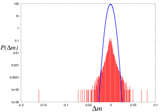
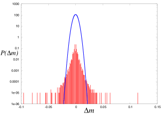
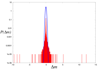
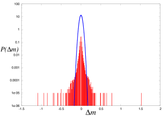
Figure 1: Empirical distributions of ‘return’ (the difference between successive mid points) $\Delta m_{t}\equiv m_{t+1}-m_{t}$ for our four kinds of data sets. From the upper left to the lower right, $P(\Delta m_{t})$ for EUR/JPY exchange rates, USD/JPY exchange rates, Nasdaq100 and price of gold are plotted. To compare the results with normal Gaussians, we calculate the empirical mean $\overline{\Delta m}\equiv(1/T)\sum_{t=0}^{T-1}\Delta m_{t}$ and the empirical variance $\overline{\sigma}_{\Delta m}^{2}\equiv(1/T)\sum_{t=0}^{T-1}(\Delta m_{t}-\overline{\Delta m})^{2}$ for each data and plot the Gaussian ${\cal N}(\overline{\Delta m},\overline{\sigma}_{\Delta m})$ in the same panel. From the upper left to the lower right, these normal Gaussians are ${\cal N}(0.000012,0.000018),{\cal N}(-0.000007,0.000013),{\cal N}(-0.000726,0.017722)$ and ${\cal N}(0.000080,0.000922)$, respectively.

We next focus on the Bid-Ask spread $S_{t}=a_{t}-b_{t}$ which is one of the key values in this study. We are confirmed that the above four data sets are classified into two types according to each statistical property of the spread. Namely, the spread of USD/JPY or EUR/JPY exchange rates is time-dependent and fluctuates, whereas, the spread of Nasdaq100 or price of gold is a time-independent constant.

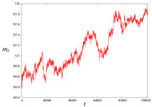
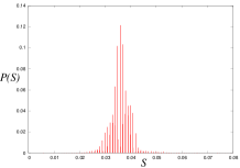
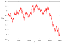
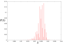
Figure 2: Statistical properties of the data set in which the spread fluctuates in time, EUR/JPY exchange rates (the upper panels) and USD/JPY exchange rates (the lower panels) are shown. From left to right, the mid point $m_{t}$, the return of the mid point $\Delta m_{t}\equiv m_{t+1}-m_{t}$ as a function of $t$, and the distribution of the spread $P(S)$ are plotted.

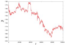
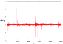
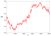
Figure 3: Statistical properties of the data set in which the spread is a time-independent constant, Nasdaq100 (the upper panels) and price of gold (the lower panels) are shown. From left to right, the mid point $m_{t}$, the return of the mid point $\Delta m_{t}\equiv m_{t+1}-m_{t}$ as a function of $t$, and the distribution of the spread $P(S)$ are plotted.

In Fig. 2 for EUR/JPY and USD/JPY exchange rates, and in Fig. 3 for Nasdaq100 and price of gold, we plot the mid point $m_{t}$, the return of the mid point $\Delta m_{t}\equiv m_{t+1}-m_{t}$ as a function of $t$ and the distribution of the Bid-Ask spread $P(S)$. From these figures, we clearly find that the Bid-Ask spread for the exchange rates apparently fluctuates, whereas the spread for Nasdaq100 or price of gold is a constant leading up to a single delta peak in the empirical distribution. From now on, the data in which the spread fluctuates is refereed to as data with stochastic Bid-Ask spread, whereas, the data in which the spread is constant is called as data with constant Bid-Ask spread. One of the main goals of this paper is to reveal the relationship between the statistical properties of Bid-Ask spread and the behaviour of auto-correlation and response functions for double-auction markets.

3 Empirical data analysis

In this section, we evaluate two macroscopic dynamical quantities, namely, auto-correlation and response functions by making use of empirical data analysis. These two relevant quantities are explicitly defined by

$$C(l) = \lim_{T\to\infty}\frac{1}{T}\sum_{t=0}^{T-1}\epsilon_{t}\epsilon_{t+l}$$ (1)

$$R(l) = \lim_{T\to\infty}\frac{1}{T}\sum_{t=0}^{T-1}\epsilon_{t}(m_{t+l}-m_{t}).$$ (2)

In order to evaluate these functions, we need the information about Selling-Buying signal $\epsilon_{t}$. However, as we mentioned in the previous section, the data gathered through the MetaTrader4 Meta does not contain any information about it explicitly. To overcome this problem, we here assume that $\epsilon_{t}$ is given in terms of ‘return’ of the mid point:

$$\epsilon_{t} = {\rm sgn}(m_{t+1}-m_{t}).$$ (3)

Namely, we assume when the mid point increases at the instant $m_{t+1}>m_{t}$, the number of traders who posted their own buying signal to the market also increases. As the result, the Selling-Buying signal $\epsilon$ is more likely to take buying $+1$ at that instant $t$.

Under the above assumption, for our four data sets, namely, EUR/JPY, USD/JPY exchange rates, Nasdaq100 and price of gold, we calculate the auto-correlation function $C(l)$ and the response function $R(l)$ via (1) and (2), respectively.

3.1 Auto-correlation function

We first plot the auto-correlation function for the above four data sets in Fig. 4.

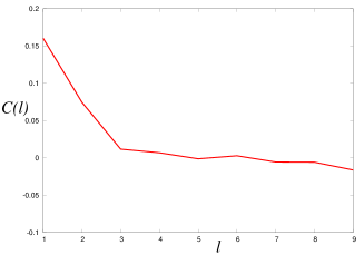
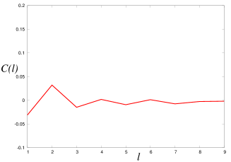
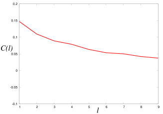
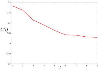
Figure 4: Typical behaviour of the auto-correlation function $C(l)$. From the upper left to the lower right, we plot EUR/JPY exchange rates (the estimated $\rho=0.24$), USD/JPY exchange rates (the estimated $\rho=0.28$), Nasdaq100 (the estimated $\rho=0.47$), price of gold (the estimated $\rho=0.51$).

From the upper left to the lower right, we plot EUR/JPY exchange rates (under the assumption on the asymptotic form: $C(l)\sim\rho^{l},\,l\gg 1$, the estimated $\rho=0.24$), USD/JPY exchange rates (the estimated $\rho=0.28$), Nasdaq100 (the estimated $\rho=0.47$ ), price of gold (the estimated $\rho=0.51$). From these panels, we find that the correlation in the Selling-Buying signals decreases in the time difference $l$ although the result for USD/JPY exchange rate possesses the negative correlation in $l=1$ and converges to zero with a slight oscillation.

3.2 Response function

We next evaluate the response function for our four data sets. The results are shown in Fig. 5.

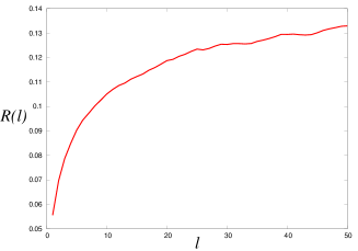
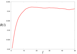
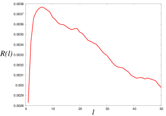
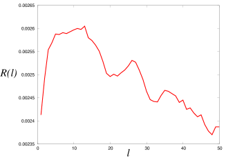
Figure 5: Typical behaviour of the response function for our empirical data: from the upper left to the lower right, the results for Nasdaq100, price of gold, EUR/JPY exchange rate and USD/JPY exchange rate are shown.

In this figure, we plot the response function for the data with stochastic Bid-Ask spread (the lower panels) and for the data with a constant Bid-Ask spread (the upper panels). From these panels, we find that some ‘non-monotonic’ behaviour in $R(l)$ appears for the data set with stochastic Bid-Ask spread.

3.3 Relationship between $C(l)$ and $R(l)$

From the definitions, both auto-correlation and response functions are functions of the time-difference $l$. In the previous subsections, we investigated their behaviour independently. However, it might be assumed that these two quantities are related each other. Therefore, it is useful for us to make ‘scatter plots’ to reveal the dynamical relationship underlying these two quantities.

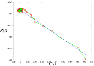
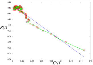
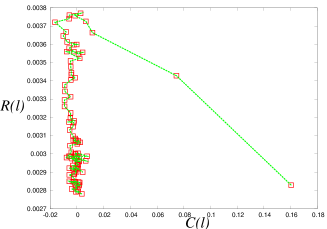
Figure 6: The relationship between $R(l)$ and $C(l)$. The upper two panels are results for the gold and Nasdaq100 with constant spreads, whereas the lower panel denotes the result for the EUR/JPY exchange rate having fluctuating spreads. We find that the linear relationship $R(l)\propto-C(l)$ holds for the data having a constant spread, whereas the linear relationship is apparently broken down in the EUR/JPY exchange rate which possesses a fluctuating Bid-Ask spread.

In Fig. 6, we plot the relationship between $R(l)$ and $C(l)$ by scatter plots. The upper two panels are results for the gold and Nasdaq100 with constant spreads, whereas the lower panel denotes the result for the EUR/JPY exchange rate having fluctuating spread. We find that the linear relationship $R(l)\propto-C(l)$ is apparently broken down in the EUR/JPY exchange rate which possesses a fluctuating Bid-Ask spread.

In the next section, we examine a phenomenological model to explain the non-linear relationship $R(l)\propto-f(C(l))$ ($f(x)$ denotes a non-linear function) theoretically.

4 A phenomenological approach

In order to explain the behaviour of the auto-correlation and response functions, we examine a phenomenological approach based on the so-called Madhavan-Richardson-Roomans model (MRR for short) MRR ; Bouchaud1 to simulate the stochastic process of price-change in empirical data sets. In the MRR model, the price $p_{t}$ updates according to the following rule.

$$p_{t+1} = p_{t}+\theta(\epsilon_{t}-\rho\epsilon_{t-1})+\xi_{t}$$ (4)

where $\xi_{t}$ denotes a noise in the market satisfying $\langle\xi_{t}\rangle=0$ and $\langle\xi_{t}\xi_{t^{{}^{\prime}}}\rangle=\delta_{t,t^{{}^{\prime}}}\Sigma^{2}$. $\theta$ is a constant value to control the slope of instantaneous price change. The label $\epsilon_{t}$ means a Selling-Buying signal to represent $\epsilon_{t}=+1$ for a buying signal and $\epsilon_{t}=-1$ vice versa.

Behaviour of the above update rule is dependent on the statistical properties of Selling-Buying signals $\epsilon_{t}$. $\rho$ is a correlation factor and in the MRR theory, we assume that $\epsilon_{t}$ follows a simple Markovian process, namely,

$$\sum_{\epsilon_{t}=\pm 1}\epsilon_{t}P(\epsilon_{t}|\epsilon_{t-1}) = \rho\epsilon_{t-1}.$$ (5)

The price value of $p_{t+1}$ provided that the Selling-Buying signal in the previous time step is $\epsilon_{t}=+1$ should be the Ask $a_{t}$ and the price $p_{t+1}$ provided that the signal is $\epsilon_{t}=-1$ should be the Bid $b_{t}$. Hence, we naturally define the time-dependence of Ask and Bid as follows.

$$a_{t} = p_{t}+\theta(1-\rho\epsilon_{t-1})+\phi$$ (6)

$$b_{t} = p_{t}+\theta(-1-\rho\epsilon_{t-1})-\phi$$ (7)

where $\phi$ denotes a kind of transaction cost and the value itself is set to a constant in the MRR model. From these rules, we easily find the Bid-Ask spread at time $t$ as

$$S_{t} = a_{t}-b_{t}=2(\theta+\phi).$$ (8)

Namely, in the MRR model, the spread is a time-independent constant during the dynamics.

On the other hand, the mid point of the Bid and Ask is given by

$$m_{t} = \frac{1}{2}(a_{t}+b_{t})=p_{t}-\theta\rho\,\epsilon_{t-1}.$$ (9)

Therefore, for the parameter choice $\theta=0$ or $\rho=0$, the mid point $m_{t}$ is identical to the price $p_{t}$. For the above update rules of price, Bid, Ask, spread and mid point, we investigate the macroscopic properties of double-auction markets through the auto-correlation function and the response function.

4.1 Auto-correlation function

From the definition of Markovian process (5), the auto-correlation function is given by

$$C(l) = \langle\epsilon_{t}\epsilon_{t+l}\rangle\equiv\sum_{\epsilon_{t}=\pm 1}\cdots\sum_{\epsilon_{t+l}=\pm 1}P(\epsilon_{t},\cdots,\epsilon_{t+l})\epsilon_{t}\epsilon_{t+l}=\rho^{l}.$$ (10)

We should keep in mind that the auto-correlation function is originally defined by (1). However, in the limit of $T\to\infty$, one can replace the time-average by the average over the joint probability of the stochastic variables $\epsilon_{t},\cdots,\epsilon_{t+l}$ as $(1/T)\sum_{t=0}^{T-1}(\cdots)=\sum_{\epsilon_{t}=\pm 1}\cdots\sum_{\epsilon_{t+l}=\pm 1}(\cdots)P(\epsilon_{t},\cdots,\epsilon_{t+l})$ according to the law of large number.

The correlation factor $\rho$ should be $|\rho|\leq 1$. For a positive $\rho$, the correlation function decays exponentially as $C(l)={\rm e}^{-l\log(1/\rho)}$.

4.2 Response function

We next consider the response function of the market, that is defined by

$$R(l) = \langle\epsilon_{t}\cdot(m_{t+l}-m_{t})\rangle$$ (11)

where the bracket $\langle\cdots\rangle$ has the same meaning as that in (10) has.

From the above response function, one obtains some information about the response of the market at time $t+l$ to the Selling-Buying signal at arbitrary time $t$. Namely, the response function measures to what extent the mid point increases (decreases) on average for interval $l$ when a buying (selling) signal is posted to the market $l$ steps before we observe the mid point. After simple algebra, we easily obtain the relationship between the response function $R(l)$ and the correlation function $C(l)$ for the MRR model as follows.

$$R(l) = \theta(1-C(l))$$ (12)

As we saw before, for a positive correlation factor $\rho>0$, the $C(l)$ monotonically decreases as $C(l)={\rm e}^{-l\log(1/\rho)}$. Hence, the response function also behaves monotonically and converges to $\theta$ as $R(l)=\theta(1-{\rm e}^{-l\log(1/\rho)})\to\theta$ ($l\to\infty$). It should be noticed that the linear relationship between $C(l)$ and $R(l)$ holds from (12).

From equation (12), we also find $R(1)=\theta(1-\rho)$ and this fact tells us that $R(\infty)/R(1)=(1-\rho)^{-1}$ holds. The volatility defined by

$$\sigma^{2}(l) \equiv \frac{1}{l}\langle(m_{t+l}-m_{t})^{2}\rangle$$ (13)

also reads

$$\sigma^{2}(l) = \Sigma^{2}+\theta^{2}(1-\rho)^{2}\left\{1+\frac{2\rho(1-\rho^{l-1})}{1-\rho}\right\}$$ (14)

and $\sigma^{2}(1)=\Sigma^{2}+\theta^{2}(1-\rho)^{2}$, $\sigma^{2}(\infty)=\Sigma^{2}+\theta^{2}(1-\rho^{2})$. We may use the above rigorous equations to check the validity of our computer simulations.

In Fig. 7, we show the typical behaviour of response function for several choices of $\rho$. From these panels, we find that for a positive correlation factor, the response function monotonically converges to the value $\theta$.

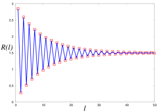
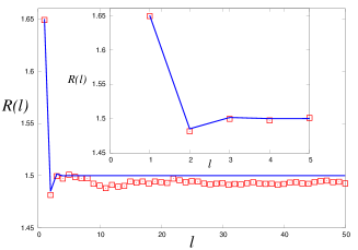
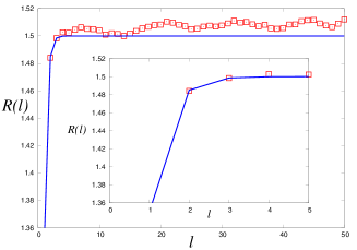
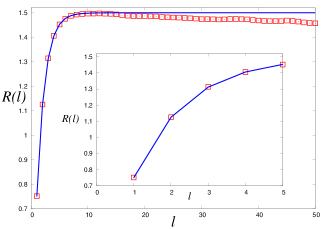
Figure 7: Typical behaviour of the response function for the MRR model. From the upper left to the lower right, we plot the response function for $\rho=-0.9,-0.1,0.1,0.5$. The solid lines are theoretical predictions by $R(l)=\theta(1-\rho^{l})$. The boxes are obtained by numerical simulations for a finite $T=10^{5}$.

In this figure, we also show the results obtained by simulating the update equation for the price (4) and the mid point (9), and calculating the response function numerically by making use of (2). We find that the both theoretical prediction (solid lines) and the simulation (boxes) are in good agreement. Moreover, for the choice of positive correlation factors, say, $\rho=0.1$ and $0.5$, the response function increases monotonically and converges to $\theta(=1.5)$ as the MRR theory predicted.

In Fig. 8, we show the relationship between $R(l)$ and $C(l)$ for the MRR model. We clearly find that the linear relationship $R(l)=\theta(1-C(l))\propto-C(l)$ actually holds. We should notice that this result is completely different from the relationship shown in the lower panel of Fig. 6 which is result for the data having fluctuating Bid-Ask spread.

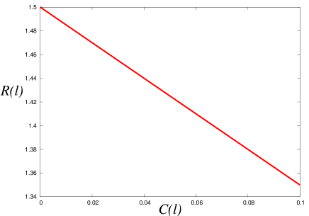
Figure 8: The relationship between $R(l)$ and $C(l)$ for the MRR model. We find that the linear relationship $R(l)=\theta(1-C(l))\propto-C(l)$ holds.

This failure of the MRR model to simulate the ‘$\lambda$-shape’ of the $C(l)$-$R(l)$ scatter plot for the data with stochastic Bid-Ask spread is obviously due to the assumption of constant Bid-Ask spread, namely, $S_{t}=a_{t}-b_{t}=2(\theta+\phi)$ on the MRR theory. We also conclude that the breaking of the linear relationship $R(l)\propto-C(l)$ is macroscopically due to the fact that the response function evaluated on the basis of the MRR theory behaves ‘monotonically’ and converges to a finite value $\theta$.

This fact is one of the limitations of the MRR theory to explain the empirical data for double-auction markets. To make the efficient model for the double-auction market with stochastic Bid-Ask spread, we use a game theoretical approach based on the so-called minority game.

5 A minority game modeling of double-auction markets

In order to make a model to simulate the ‘non-monotonic’ behaviour of the response function for the financial data with stochastic Bid-Ask spread, we start our argument from standard minority game Arthur ; Challet1997 ; Challet ; Coolen with a finite market history length.

5.1 General set-up

In our computer simulations for the minority game, at each round $t$ (time step) of the game, each trader $i$ ($i=1,\cdots,N$: $N$ should be an odd number to determine the ‘minority group’) decides his (or her) decision: ${\cal B}_{i}(t)=+1$ (buy) or ${\cal B}_{i}(t)=-1$ (sell) to choose the minority group. Then, we evaluate the total decision of the traders:

$$A(t) = \frac{1}{\sqrt{N}}\sum_{i=1}^{N}{\cal B}_{i}(t)$$ (15)

for each round $t$. It should be noted that the factor $N^{-1/2}$ is needed to make the $A(t)$ of order $1$ object (independent of the size $N$). From the definition (15), the market is seller’s market for $A(t)>0$, whereas the market behaves as buyer’s market for $A(t)<0$. The $A(t)$ follows complicated stochastic process and one might consider that the price $p$ is updated in terms of the $A(t)$ as follows.

$$p(t+1) = p(t)+\beta\{A(t)+\psi\,{\rm sgn}[A(t-1)]\}$$ (16)

where $\beta$ and $\psi$ are positive constants. The above update rule means that the price increases if the ‘buying group’ is majority and decreases vice versa. This setting of the game seems to be naturally accepted. A bias term $\psi$ appearing in (16) plays an important role to simulate the auto-correlation function as we will see later on.

To decide ‘buy’ or ‘sell’, each trader uses the following information vector defined by

$$\mbox{\boldmath$\lambda$}(A,Z:t) = \left(\begin{array}[]{c}{\rm sgn}[(1-\zeta)A(t-1)+\zeta Z(t,1)]\\ {\rm sgn}[(1-\zeta)A(t-2)+\zeta Z(t,2)]\\ \cdots\\ {\rm sgn}[(1-\zeta)A(t-M)+\zeta Z(t,M)]\end{array}\right)$$ (21)

where ${\rm sgn}(x)$ denotes a sign function and $Z(t,\xi),\xi=1,\cdots,M$ is a white noise defined by

$$\langle Z(t,\xi)Z(t^{{}^{\prime}},\xi^{{}^{\prime}})\rangle = \delta_{t,t^{{}^{\prime}}}\delta_{\xi,\xi^{{}^{\prime}}}.$$ (22)

Therefore, each trader uses the information of market through the up-down configuration of the return $A$ (with some additive noise $Z$) back to the previous $M$-steps. If the $\zeta$ is close to $1$, the ‘real’ market history through the $A$ is hided by the ‘fake’ market history through the noise $Z$.

For a given information vector $\mbox{\boldmath$\lambda$}(A,Z:t)=\mbox{\boldmath$\lambda$}$ chosen from all possible $2^{M}$ candidates, each trader $i$ decides her (or his) action at round $l$ by the following strategy vector:

$$\mbox{\boldmath$r$}_{\Lambda}^{i} = (r_{\Lambda}^{i1},\cdots,r_{\Lambda}^{is}),\,\,\,\Lambda=1,\cdots,2^{M}$$ (23)

where we defined $\Lambda$ as the index (entry) of the selected information vector $\lambda$ and $s$ stands for the number of the possible strategies for each trader. Each component of the above strategy vector $\mbox{\boldmath$r$}_{\Lambda}^{i}$ takes $+1$ (buy) or $-1$ (sell). Therefore, each trader has her (his) own look-up table which is defined by a matrix with size $s\times 2^{M}$ as

$$\mbox{\boldmath$R$}^{i}\equiv\left(\begin{array}[]{c}\mbox{\boldmath$r$}_{1}^{i}\\ \mbox{\boldmath$r$}_{2}^{i}\\ \cdot\\ \cdot\\ \cdot\\ \mbox{\boldmath$r$}_{2^{M}}^{i}\end{array}\right) = \left(\begin{array}[]{cccc}r_{1}^{i1}&r_{1}^{i2}&\cdots&r_{1}^{is}\\ r_{2}^{i1}&r_{2}^{i2}&\cdots&r_{2}^{is}\\ \cdots&\cdots&\cdots&\cdots\\ \cdots&\cdots&\cdots&\cdots\\ \cdots&\cdots&\cdots&\cdots\\ r_{2^{M}}^{i1}&r_{2^{M}}^{i2}&\cdots&r_{2^{M}}^{is}\end{array}\right).$$ (36)

Each component of the above look-up table $r_{\Lambda}^{is}=\{+1,-1\}$ is fixed (‘quenched’) before playing the game. However, in the next section, we consider the case in which the components of look-up tables are rewritten during the game. In this paper, we concentrate ourselves to the simplest case of two strategies $s=2$ and $\zeta=0$ (‘real’ market history). Then, the trader $i$ changes her/his own pay-off value ${\cal P}_{ic}$ by the following update rule:

$${\cal P}_{ic}(t+1) = {\cal P}_{ic}(t)-\frac{1}{\sqrt{N}}{\cal B}_{i}(t)A(t)$$ (37)

$${\cal B}_{i}(t) = \sum_{\Lambda=1}^{2^{M}}\delta(\Lambda,\mbox{\boldmath$\lambda$}(A,Z:t))r_{\Lambda}^{i\tilde{c}_{i}(t)}$$ (38)

where $\delta(x,y)$ denotes the Kronecker’s delta and $\tilde{c}_{i}(t)$ means the optimal strategy in the sense that $\tilde{c}_{i}(t)$ is given by

$$\tilde{c}_{i}(t) = {\arg\max}_{c}[{\cal P}_{ic}(t)].$$ (39)

The meaning of the update rule (37) is given as follows. If $A(t)>0$ and the majority group consists of traders who post their decisions $+1$ to the market, the trader $i$ attempts to post her/his decision as an opposite sign of $A(t)$, namely, ${\cal B}_{i}(t)=-1$. Thus, the trader $i$ acts so as to satisfy the condition ${\cal B}_{i}(t)A(t)<0$ which leads to increase of her/his pay-off value ${\cal P}_{ic}(t+1)$.

By taking into account the fact that we are dealing with the case of $s=2$ ($c=1,2$), we rewrite the equation (37) as

$$q_{i}(t+1) = q_{i}(t)-\frac{1}{\sqrt{N}}\sum_{\Lambda=1}^{2^{M}}\delta(\Lambda,\mbox{\boldmath$\lambda$}(A,Z:t))\eta_{\Lambda}^{i}A(t)$$ (40)

by means of

$$q_{i}(t) = \frac{1}{2}({\cal P}_{i1}(t)-{\cal P}_{i2}(t)),\,\,\,\,\eta_{\Lambda}^{i}=\frac{1}{2}(r_{\Lambda}^{i1}-r_{\Lambda}^{i2}).$$ (41)

Substituting (38) into the definition of the total bit $A(t)$, we have

$$A(t) = \frac{1}{\sqrt{N}}\sum_{i=1}^{N}{\cal B}_{i}(t)=\frac{1}{\sqrt{N}}\sum_{i=1}^{N}\sum_{\Lambda=1}^{2^{M}}\delta(\Lambda,\mbox{\boldmath$\lambda$}(A,Z:t))r_{\Lambda}^{i\tilde{c}_{i}(t)}.$$ (42)

We should notice that the above equation can be written by using the following relation

$$r_{\Lambda}^{i\tilde{c}_{i}(t)} = w_{\Lambda}^{i}+{\rm sgn}[q_{i}(t)]\eta_{\Lambda}^{i},\,\,\,w_{\Lambda}^{i}=\frac{1}{2}(r_{\Lambda}^{i1}+r_{\Lambda}^{i2}).$$ (43)

Then, we obtain the following coupled non-linear equations with respect to the total decision $A(t)$, the difference of pay-off values for two strategies $q_{i}(t)$ and the update equation of the price $p(t)$:

$$A(t) = \frac{1}{\sqrt{N}}\sum_{i=1}^{N}\sum_{\Lambda=1}^{2^{M}}\delta(\Lambda,\mbox{\boldmath$\lambda$}(A,Z:t))\left\{w_{\Lambda}^{i}+{\rm sgn}[q_{i}(t)]\eta_{\Lambda}^{i}\right\}$$ (44)

$$q_{i}(t+1) = q_{i}(t)-\frac{1}{\sqrt{N}}\sum_{\Lambda=1}^{2^{M}}\delta(\Lambda,\mbox{\boldmath$\lambda$}(A,Z:t))\eta_{\Lambda}^{i}A(t)$$ (45)

$$p(t+1) = p(t)+\beta\{A(t)+\psi\,{\rm sgn}[A(t-1)]\}.$$ (46)

The above rules (45)(44) and (46) are our basic equations to discuss the response of double-auction markets having stochastic Bid-Ask spread to instantaneous Selling-Buying signals.

5.2 Making of the Bid-Ask spread in the minority game

To make the Bid-Ask spread in our minority game, we assume that the buying price $a_{it}$ and the selling price $b_{it}$ which are posted to the market by each trader $i$ at round (time) $t$ are updated according to the following rules.

$$a_{it} = p(t)+\gamma_{a}\,g_{it}+\delta$$ (47)

$$b_{it} = p(t)+\gamma_{b}\,g_{it}-\delta$$ (48)

where $\gamma_{a},\gamma_{b}$ and $\delta$ are constants to be set so as to satisfy $a_{it}-b_{it}>0$. $g_{it}$ is an uncorrelated Gaussian variable with mean $\langle g_{it}\rangle=0$ and covariance $\langle g_{it}g_{i^{{}^{\prime}}t^{{}^{\prime}}}\rangle=\delta_{t,t^{{}^{\prime}}}\delta_{i,i^{{}^{\prime}}}$ (additive white Gaussian noise: AWGN). In our simulations, we set $\gamma_{a}=\gamma_{b}=0.01,\delta=0.049$. Then, the Bid-Ask spread at round $t$ is given by

$$S_{t} = {\min}\{a_{it}|a_{it}\in N_{+}\}-{\max}\{b_{it}|b_{it}\in N_{-}\}$$ (49)

where the groups taking ‘buying’ and ‘selling’ decisions are refereed to as $N_{+}$ and $N_{-}$, respectively ($N\equiv N_{+}+N_{-}$).

In Fig. 9, we plot the resulting distribution of the spread $S=S_{t}$.

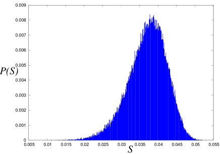
Figure 9: Distribution of the spread $S=S_{t}$ generated by the minority game.

From Fig. 9, we find that the stochastic Bid-Ask spread generated from the above modeling based on the minority game actually fluctuates and possesses a non-trivial shape of the distribution.

5.3 Results

For the above set-up of the minority game, we evaluate two relevant statistics, namely, correlation function $C(t)$ (by (1)) and the response function $R(t)$ (by (2)) to compare the results with the empirical evidence for the data with stochastic Bid-Ask spread.

5.3.1 Auto-correlation function

We first examine the effect of the bias term $\psi$ on the correlation function. The results for $\psi=0$ are shown in Fig. 10 (left).

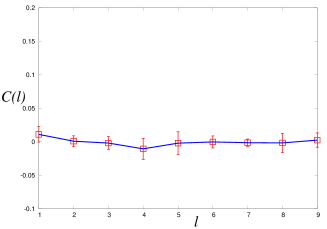
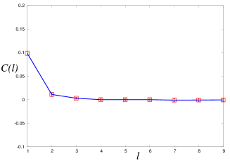
Figure 10: Auto-correlation function $C(l)$ in the minority game for $\psi=0$ (left). We set $N=1025,M=9,\beta=0.01$ and iterated the game $100010$ rounds. The $C(l)$ is zero for $l\geq 2$. The right panel is auto-correlation function of the MRR model with $\rho=0.1$. The error-bars were calculated by 10-independent trials.

From this panel, we find that $C(l)=0$ for $l\geq 2$ and the result is apparently different from the result for the empirical data. Here we set $N=1025,M=9,\beta=0.01$ and iterated the game $t=100010$ rounds. The right panel of Fig. 10 shows the correlation function of the MRR model for $\rho=0.1$. The Selling-Buying signal

$$\epsilon_{t} = {\rm sgn}[A(t)]$$ (50)

is actually correlated automatically through the market history with length $M=9$, however, the correlation strength is very weak. Therefore, we need some other explicit correlation through the bias term $\psi$ which enhances the correlation by two-round back $A(t-1)$ from the present $t+1$. Hence, we here choose the non-zero bias term $\psi$ to reproduce the auto-correlation function as observed in the empirical data.

We checked that the results are robust against the slight differences in the parameters appearing in the game such as $\beta,M,\delta$ etc. However, for only parameter $\psi$, we should be careful to choose the value. This is because from the definition of update rule of the price (46), the effect of the $A(t)$ on the price change is relatively depressed by the large value of the $\psi$. Therefore, we should choose $\psi$ so as to make the value smaller than the standard deviation of the $A(t)$, namely, square root of the volatility as

$$\psi < \sqrt{\frac{1}{T}\sum_{t=1}^{T}\{A(t)-\overline{A(t)}\}^{2}}\equiv\sigma_{A}.$$ (51)

In our simulation, the square root of the volatility is estimated as $\sigma_{A}=0.44295$. In Fig. 11, we plot the correlation function for the case of $\psi=0.05$ (left panel) and $\psi=0.1$ (right). We should notice that these two choices of the bias term $\psi$ satisfy the condition (51).

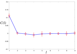
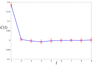
Figure 11: Auto-correlation function $C(l)$ in the minority game for $\psi=0.05$ (left) and $\psi=0.1$ (right). We set $N=1025,M=9,\beta=0.01$ and iterated the game for $100010$ rounds. The error-bars were calculated by 10-independent trials.

From these panels, we find that the correlation function decreases as we observed in the same function for the empirical data sets.

5.3.2 Response function

We next plot the response function in Fig. 12 for $\psi=0.$(upper panel), $\psi=0.05$ (lower left) and $\psi=0.1$ (lower right).

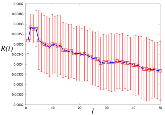
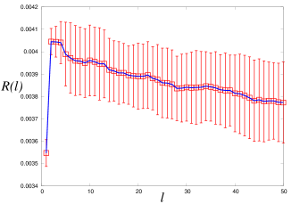
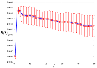
Figure 12: Response function $R(l)$ in the minority game for $\psi=0$ (upper), $\psi=0.05$ (lower left) and $\psi=0.1$ (lower right). We set $N=1025,M=9,\beta=0.01$ and iterated the game for $100010$ rounds. The error-bars were calculated by 10-independent trials.

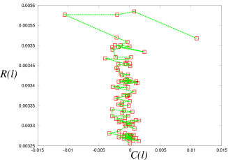
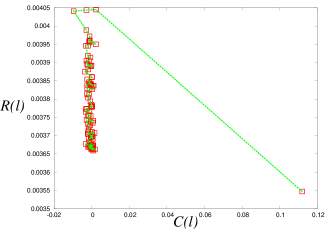
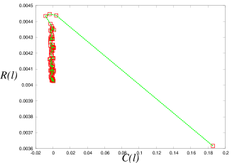
Figure 13: The relationship between $C(l)$ and $R(l)$ for minority game with $\psi=0$ (upper), $\psi=0.05$ (lower left) and $\psi=0.1$ (lower right). We set $N=1025,M=9,\beta=0.01$ and iterated the game for $100010$ rounds and we calculate $C(l),R(l)$ up to $l=100$.

From these panels, we find that the behaviour of the response function is not monotonically increasing function leading up to the convergence to some constant value but ‘non-monotonic’ as the response function of data sets having stochastic Bid-Ask spread (EUR/JPY, USD/JPY exchange rates) shows (see the lower panels of Fig. 5).

5.3.3 Relationship between the auto-correlation and response functions

In Fig. 13, we plot the relationship between the auto-correlation and response functions. In the upper panel, we show the result for zero bias term $\psi=0$. we find that the curve is deviated from the linear relation $R(l)\propto-C(l)$. However, the shape is not ‘$\lambda$’ as observed in the empirical evidence but ‘$T$-shape’. In the lower two panels are results for the non-zero bias term $\psi\neq 0$. We clearly find that the ‘$\lambda$-shapes’ appears and the results are qualitatively similar to those of the empirical data.

6 Adaptive look-up tables

In the previous section, we fixed each decision component (buying: $+1$, selling: $-1$) in their look-up tables before playing the game (in this sense, the decision components are ‘quenched variables’ in the literature of disordered spin systems such as spin glasses). However, in this paper, a certain amount of traders update their decision components according to the macroscopic market history (they ‘learn’ from the behaviour of markets) so as to be categorized into two-groups with a finite probability (in this sense, the components are now regarded as ‘annealed variables’). Namely, at each round of the game, if the number of sellers is smaller/greater than that of buyers, a fraction of traders, what we call optimistic group/pessimistic group, is more likely to rewrite their own decision components from $-1$/$+1$ to $+1$/$-1$. In realistic trading, we might change our mind and rewrite the components of the look-up table according to the market history. Therefore, in this section we consider the case in which some amount of traders can rewrite their own table adaptively.

6.1 Adaptation using the latest market information

We first consider the case in which each trader updates her/his own look-up table according to the latest information of the market. Some of the traders make their decisions as ‘buy’ when the market is seller’s market, namely, the signal of the latest market is ‘buying’ (what we call optimistic group). On the other hand, they decide ‘sell’ vice versa (they are referred to as pessimistic group). Namely, each trader rewrites the table according to the following algorithm.

Adaptation algorithm using the latest market information

1. Fix (‘quench’) each component of the look-up table at the beginning of the game $t=-M$.

2. At each game round $t$ for $t>-M$, each trader rewrites her/his component $r_{\Lambda}^{i1},r_{\Lambda}^{i2}$, where $\Lambda$ denotes the entry of market history for the information vector $\mbox{\boldmath$\lambda$}(A,Z:t)$, with probability $f_{1}$ as

   $$r_{\Lambda}^{i1}={\rm sgn}[(A(t-1)],\,\,\,r_{\Lambda}^{i2}={\rm sgn}[A(t-1)].$$

3. Each trader recovers her/his original (at the beginning of the game) look-up table with a probability $f_{2}$ at the next game round $t+1$.

4. Repeat (ii) and (iii) until the game is over.

Namely, a fraction $\sim Nf_{1}$ of the traders is categorized into the ‘optimistic group’ if $A(t-1)>0$ (seller’s market) and into the ‘pessimistic group’ if $A(t-1)<0$ (buyer’s market).

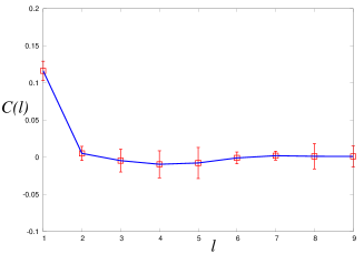
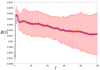
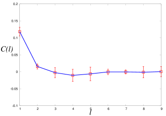
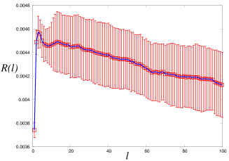
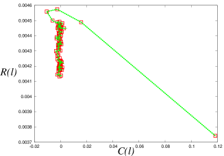
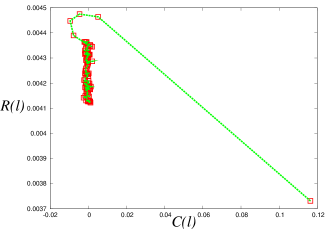
Figure 14: Dynamical quantities $C(l)$ (upper left, middle left) and $R(l)$ (upper right, middle right) evaluated for the minority game with adaptive look-up tables. We set $\psi=0,f_{1}=0.01$. $f_{2}=1$ (upper panels), $f_{2}=0.9$ (middle panels). The lower two panels show the relationship between the auto-correlation and response functions for $(f_{1},f_{2})=(0.01,1)$ (left) and $(f_{1},f_{2})=(0.01,0.9)$ (right).

6.1.1 Results

In Fig. 14, we show dynamical quantities $C(l)$ (upper left, middle left) and $R(l)$ (upper right, middle right) evaluated for the minority game with adaptive look-up tables. We set $\psi=0,f_{1}=0.01$ and $f_{2}=1$ (upper panels), $f_{2}=0.9$ (middle panels). The lower two panels show the relationship between the auto-correlation and response functions for $(f_{1},f_{2})=(0.01,1)$ (left) and $(f_{1},f_{2})=(0.01,0.9)$ (right). From this figure, we find that the positive correlation $C(l)>0$ for $l=1$ appears even if we set $\psi=0$ and non-monotonic behaviour of the response function is reproduced. As the result, ‘$\lambda$-shape’ in the $C(l)$-$R(l)$ scatter plots is generated. From these results, we conclude that the adaptive modification of the look-up table by using the latest market information for each trader works well to explain the empirical evidence.

6.2 Adaptation by using the market history

In the previous subsection, we succeeded in generating a positive finite auto-correlation by making use of the adaptive look-up table even if we set $\psi=0$. However, in this look-up table, each trader changes her/his decision from the latest information about the market. As the result, the auto-correlation function decays to zero for $l\geq 2$. To modify the weak correlation, we construct the adaptive look-up table by using the information about the market history with length $M$. As we mentioned, the information vector $\mbox{\boldmath$\lambda$}(A,Z:t)$ contains the useful information on the market. Hence, we shall assume that each trader rewrites the component of her/his table as

$$r_{\Lambda}^{i1}={\rm sgn}[\Omega_{\Lambda}(A,Z:t)],\,\,\,r_{\Lambda}^{i2}={\rm sgn}[\Omega_{\Lambda}(A,Z:t)]$$ (52)

with probability

$$f_{3} = \frac{\alpha|\Omega_{\Lambda}(A,Z:t)|}{2^{M}}$$ (53)

where we defined

$$\Omega_{\Lambda}(A,Z:t) \equiv \mbox{\boldmath$w$}\cdot\mbox{\boldmath$\lambda$}(A,Z:t)=\sum_{\tau=1}^{M}2^{M-\tau}{\rm sgn}[A(t-\tau)]$$ (54)

$$w \equiv (2^{M-1},2^{M-2},\cdots,2^{0})$$ (55)

at each game round $t$. We should keep in mind that each trader recovers her/his original look-up table with a probability $f_{2}$ at the next game round. The $\Omega_{\Lambda}(A,Z:t)$ denotes cumulative weighted market status, namely, we assume that the importance of the market information decays as $2^{-\tau}$ in the history length $\tau$.

For instance, for the information vector (let us define the entry by $\Lambda$) having $+1$ for all components: $\mbox{\boldmath$\lambda$}(A,Z:t)=({\rm sgn}[A(t-1)],\cdots,{\rm sgn}[A(t-M)])=(+1,\cdots,+1)$, that is, the market remains as seller’s market up to $M$-times back, we obtain $\Omega_{\Lambda}(A,Z:t)=2^{M}-1>0$ and $Nf_{3}=N\alpha(1-2^{-M})$-traders rewrite their components as $r_{\Lambda}^{i1},r_{\Lambda}^{i2}={\rm sgn}[\Omega_{\Lambda}(A,Z,t)]=1$. As another example, when seller’s market and buyer’s market appears periodically as $\mbox{\boldmath$\lambda$}(A,Z:t)=(-1,+1,-1,+1,\cdots)$, we have $\Omega_{\Lambda}(A,Z:t)=-\{2^{M}-(-1)^{M}/2\}/3<0$ and $Nf_{3}=N\alpha\{1-(-1)^{M}/2^{M+1}\}/3$-traders rewrite their component as $r_{\Lambda}^{i1},r_{\Lambda}^{i2}={\rm sgn}[\Omega_{\Lambda}(A,Z:t)]=-1$.

Let us summarize the above procedure as the following algorithm.

Adaptation algorithm using the market history

1. Fix (‘quench’) each component of the look-up table at the beginning of the game $t=-M$.

2. At each game round $t$ for $t>-M$, each trader rewrites her/his component $r_{\Lambda}^{i1},r_{\Lambda}^{i2}$, where $\Lambda$ denotes the entry of market history for the information vector $\mbox{\boldmath$\lambda$}(A,Z:t)$, with probability as

   $$r_{\Lambda}^{i1}={\rm sgn}[\Omega_{\Lambda}(A,Z:t)],\,\,\,r_{\Lambda}^{i2}={\rm sgn}[\Omega_{\Lambda}(A,Z,t)]$$

   with probability

   $$f_{3}=\frac{\alpha|\Omega_{\Lambda}(A,Z:t)|}{2^{M}}$$

   with $\Omega_{\Lambda}(A,Z:t)=\sum_{\tau=1}^{M}2^{M-\tau}{\rm sgn}[A(t-\tau)]$.

3. Each trader recovers her/his original (at the beginning of the game) look-up table with a probability $f_{2}$ at the next game round $t+1$.

4. Repeat (ii) and (iii) until the game is over.

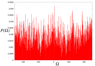
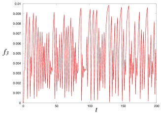
Figure 15: The generated distribution $P(\Omega)$ of $\Omega_{\Lambda}(A,Z:t)=\Omega$ (left) and the typical time-evolution of the probability $f_{3}$ for the first $200$-steps (right).

We set $\alpha=0.01$ and select the same values as those of the previous section for the other parameters.

6.2.1 Results

In Fig. 15, we first plot the generated distribution $P(\Omega)$ of $\Omega_{\Lambda}(A,Z:t)=\Omega$ (left) and the typical time-evolution of the probability $f_{3}$ for the first $200$ steps (right). It should be noted that $\Omega$ in the left panel is ranged from $\Omega_{\rm min}=\sum_{\tau=1}^{M}2^{M-\tau}(-1)=1-2^{9}=-511$ to $\Omega_{\rm max}=\sum_{\tau=1}^{M}2^{M-\tau}(+1)=2^{9}-1=511$ because we set the history length $M=9$ in the definition of the $\Omega_{\Lambda}(A,Z:t)$. We find from the right panel that the typical time-evolution of the probability $f_{3}$ obeys complicated dynamics.

We next show the results for the macroscopic quantities in Fig. 16.

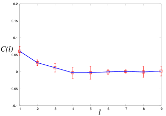
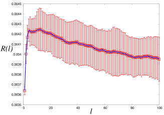
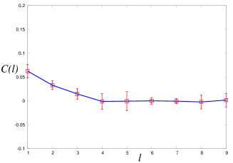
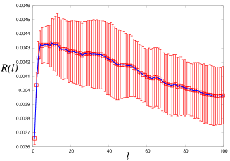
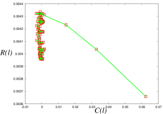
Figure 16: Dynamical quantities $C(l)$ (upper left, middle left) and $R(l)$ (upper right, middle right) evaluated for the minority game with adaptive look-up tables for $M$ market history length. We set $\psi=0$, $f_{2}=1$ (upper panels), $f_{2}=0.9$ (middle panels). The lower two panels show the relationship between the auto-correlation and response functions for $f_{2}=1$ (left) and $f_{2}=0.9$ (right).

From this figure, we confirm that the ‘$\lambda$-shape’ in $R(l)$-$C(l)$ scatter plots are much similar to the empirical evidence than the results in the previous subsection.

7 Discussion

Our general set-up presented in this paper is applicable to the analysis for the other quantities or for the other stochastic models. Here we shall mention them briefly.

7.1 Waiting time statistics

As we mentioned in section 1, we can generate the duration between the price changes within the framework of our minority game.

Let us introduce the maximum value of the spread $\bar{S}$ which is determined by market makers. Then, we might define a set of time points at which the price is updated as

$$\{t\} \equiv \{t_{k}|S_{t_{k}}=\min\{a_{it_{k}}|a_{it_{k}}\in N_{+}\}-\max\{b_{it_{k}}|b_{it_{k}}\in N_{-}\}<\bar{S}\}$$ (56)

For these time points $t_{k}$, the duration between successive price changes is given by

$$\{\tau\} \equiv \{\tau_{k}|\tau_{k}=t_{k+1}-t_{k}\}$$ (57)

We can evaluate the distribution $P(\tau)$ and compare the results with well-known distributions, for instance, the Mittag-Leffler type Enrico ; anowaiting ; Enrico06 .

7.2 Mean-field models

Recently, Vikram and Sinha Sinha proposed a mean-field model to describe the collective behaviour of financial markets. In their model, each trader $i$ decides his (her) decision: $S_{i}(t)=+1$ (buy), $-1$ (sell) and $S_{i}(t)=0$ (no action) at time $t$ according to the following probability.

$$P[|S_{i}(t)|=1]=1-P[S_{i}(t)=0] = {\exp}\left(-\mu{\Biggr{|}}\log\frac{p(t)}{\langle p(t)\rangle_{\tau}}{\Biggr{|}}\right)$$ (58)

where $p(t)$ stands for the price at time $t$ and the bracket $\langle\cdots\rangle_{\tau}$ means the moving average over the past $\tau$-time steps. The parameter $\mu$ is a parameter which controls the sensitivity of an agent to the magnitude of deviation of the price from its moving average $\langle p(t)\rangle$. For $\mu=0$, the system reduces to a binary decision model where every agent trades at all time instants. Namely, $P[S_{i}(t)=0]=0$ for $\mu=0$ means that the trader decides his (her) action, buy or sell, certainly. The traders who decide to trade at $t$ make his (her) action randomly, that is, $P[S_{i}(t)=1]=P[S_{i}=-1]=1/2$. The price at time $t+1$ is decided by the following recursion relation.

$$p(t+1) = \left(\frac{1+A_{t}}{1-A_{t}}\right)p(t)$$ (59)

where $A_{t}\equiv(1/\sqrt{N})\sum_{i=1}^{N}S_{i}(t)$. In Fig.17, we plot the typical time-evolution of the price $p(t)$ and the moving average $\langle p(t)\rangle_{\tau}$ evaluated by (58) and (59).

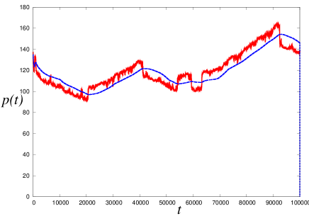
Figure 17: Typical behaviour of time evolution of the price $p(t)$ (the solid line) and the moving average $\langle p(t)\rangle_{\tau}$ (the broken line) evaluated by (58) and (59). We set $\mu=100,\tau=10000$.

To construct the double-auction market for the above price change, we shall use the same definitions of buying $b_{it}$ and selling $a_{it}$ signals for each trader $i$ at time $t$ as (47)(48) in our minority game modeling. Then, we calculate the response function and the auto-correlation function by using the above set-up and plot them in Fig. 18.

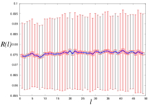
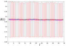
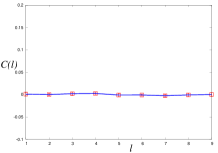
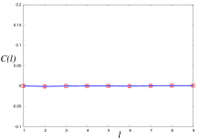
Figure 18: Typical behaviour of the response function (upper panels) and the auto-correlation function (lower panels) for the Vikam-Sinha model. From the left to the right, we set $(\mu,\tau)=(100,10000),(10,10000),(100,1000)$. The error-bars were calculated by 10-independent trials.

We set the number of agents $N=20000$, the number of iterations for the price change $T=100000$. We also choose $\delta=0.02,\gamma_{a}=\gamma_{b}=0.001$. The initial condition on the price $p(t)$ is chosen from the Eur/JPY exchange rate in the empirical data. From this figure, we find that the behaviour is different from the empirical evidence. Especially, the auto-correlation function fluctuates with very large amplitudes. This result might come from the fact that in the Vikam-Sinha model, the buying-selling signal is chosen randomly. Therefore, we should modify the Vikram-Sinha model in order to explain the non-monotonic behaviour of the response function in double-auction markets with stochastic Bid-Ask spread.

8 Summary

In this paper, statistical properties of double-auction markets with Bid-Ask spread were investigated through the response function. We first attempted to utilize the so-called Madhavan-Richardson-Roomans model (MRR for short) to simulate the stochastic process of the price-change in empirical data sets (say, EUR/JPY or USD/JPY exchange rates) in which the Bid-Ask spread fluctuates in time. We found that the MRR theory apparently does not simulate so much as the qualitative behaviour (‘non-monotonic’ behaviour) of the response function calculated from the data. Especially, we were confirmed that the stochastic nature of the Bid-Ask spread causes apparent deviations from a linear relationship between the $R(l)$ and the auto-correlation function $C(l)$, namely, $R(l)\propto-C(l)$. To make the microscopic model of double-auction markets having stochastic Bid-Ask spread, we utilized the minority game with a finite market history length and found numerically that appropriate extension of the game shows quite similar behaviour of the response function to the empirical evidence. We also revealed that the minority game modeling with the adaptive (‘annealed’) look-up table reproduces the non-linear relationship $R(l)\propto-f(C(l))$ ($f(x)$ stands for a non-linear function leading to ‘$\lambda$-shapes’) more effectively than fixed (‘quenched’) look-up table does.

Of course, there are still gaps between the theoretical prediction and the empirical evidence. We should modify our modeling of the double-auction market and figure out the micro-macro relationship in the market much more quantitatively.

References

- (1) M. O’hara, Market Microstructure Theory, (Blackwell Publishing) (1995).
- (2) http://moneykit.net/
- (3) S. Redner, A Guide to First-Passage Processes, Cambridge University Press (2001).
- (4) N.G. van Kappen, Stochastic Processes in Physics and Chemistry, North Holland, Amsterdam (1992).
- (5) M. Montero and J. Masoliver, European Journal of Physics B 57, 181 (2007).
- (6) N. Sazuka, Physica A 376, pp. 500-506 (2007).
- (7) N. Sazuka and J. Inoue, Physica A 383, pp. 49-53 (2007).
- (8) J. Inoue and N. Sazuka, Physical Review E 76, pp. 021111 (9 pages) (2007).
- (9) N. Sazuka and J. Inoue, Proceedings of the IEEE Symposium Series on Computational Intelligence (FOCI2007), Devid Fogel (Eds.), pp. 416-423 (2007).
- (10) N. Sazuka, J. Inoue and E. Scalas, Physica A 388, pp. 2839-2853 (2009).
- (11) J. Inoue and N. Sazuka, Quantitative Finance 10, pp. 121-130 (2010).
- (12) J. Inoue, N. Sazuka and E. Scalas, Science Culture 76, No.9-10, pp. 466-470 (2010).
- (13) J. Inoue, H. Hino, N. Sazuka and E. Scalas, in preparation.
- (14) R.J. Elliott and K. Ekkehard, Mathematics of Financial Markets, (New York: Springer) (2004).
- (15) A. Madhavan, M. Richerdson and M. Roomans, The Review of Financial Studies 10, No. 4, pp. 1035-1064 (1997).
- (16) M. Wyart, J.-P. Bouchaud, J. Kockelkoren, M. Potters and M. Vettorazzo, Quantitative Finance 8, pp.41-57 (2008).
- (17) J.-P. Bouchaud, J. Kockelkoren and M. Potters, Quantitative Finance 6, pp.115-123 (2006).
- (18) A. Ponzi, F. Lillo and R. N. Mantegna, Physical Review E 80, 016112 (2009).
- (19) M. Mezard, G. Parisi and M.A. Virasoro, Spin Glass Theory and Beyond, World Scientific Singapore (1987).
- (20) http://www.metaquotes.net/
- (21) J.-P. Bouchaud and M. Potters, Theory of Financial Risk and Derivative Pricing, (Cambridge: Cambridge University Press) (2000).
- (22) W. B. Arthur, Inductive Reasoning and Bounded Rationarity (The El Farol Problem), Am. Econ. Rev., 84, pp. 488-500 (1994).
- (23) D. Challet and Y.-C. Zhang, Physica A 246, pp.407-418 (1997).
- (24) D. Challet, M. Marsili and Y.-C. Zhang, Minority Games, (Oxford: Oxford University Press) (2005).
- (25) A.C.C. Coolen, The Mathematical Theory Of Minority Games: Statistical Mechanics Of Interacting Agents, (Oxford: Oxford University Press) (2005).
- (26) E. Scalas, Chaos, Soliton Fractals 34, 33 (2007).
- (27) E. Scalas, R. Gorenflo, H. Luckock, F. Mainardi, M. Mantelli, and M. Raberto, Quantitative Finance, 4, 695 (2004).
- (28) E. Scalas, T. Kaizoji, M. Kirchler, J. Huber, and A. Tedeschi, Physica A, 366, 463 (2006).
- (29) E. Scalas, http://arxiv.org/abs/physics/0608217.
- (30) S.V. Vikram and S. Sinha, Physical Review E 83, 016101(2010).