The Last Eight-Billion Years of Intergalactic Si IV Evolution

Abstract

We identified 24 Si IV absorption systems with $z\lesssim 1$ from a blind survey of 49 low-redshift quasars with archival Hubble Space Telescope ultraviolet spectra. We relied solely on the characteristic wavelength separation of the doublet to automatically detect candidates. After visual inspection, we defined a sample of 20 definite (group G = 1) and 4 “highly-likely” (G = 2) doublets with rest equivalent widths $W_{r}$ for both lines detected at $\geq 3\sigma_{W_{r}}$. The absorber line density of the G = 1 doublets was $\mathrm{d}\mathcal{N}_{\mathrm{Si\,IV}}/\mathrm{d}X=1.4^{+0.4}_{-0.3}$ for $\log N(\mathrm{Si}^{+3})>12.9$. The best-fit power law to the G = 1 frequency distribution of column densities $f(N(\mathrm{Si}^{+3}))$ had normalization $k=(1.2^{+0.5}_{-0.4})\times 10^{-14}\,{\rm cm}^{2}$ and slope $\alpha_{N}=-1.6^{+0.3}_{-0.3}$. Using the power-law model of $f(N(\mathrm{Si}^{+3}))$, we measured the $\mathrm{Si}^{+3}$ mass density relative to the critical density: $\Omega_{\mathrm{Si}^{+3}}=(3.7^{+2.8}_{-1.7})\times 10^{-8}$ for $13\leq\log N(\mathrm{Si}^{+3})\leq 15$. From Monte Carlo sampling of the distributions, we estimated our value to be a factor of $4.8^{+3.0}_{-1.9}$ higher than the $2\leq z\leq 4.5$ $\langle\Omega_{\mathrm{Si}^{+3}}\rangle$. From a simple linear fit to $\Omega_{\mathrm{Si}^{+3}}$ over the age of the Universe, we estimated a slow and steady increase from $z=5.5\rightarrow 0$ with $\mathrm{d}\Omega_{\mathrm{Si}^{+3}}/\mathrm{d}t_{\rm age}=(0.61\pm 0.23)\times 10^{-8}\,{\rm Gyr}^{-1}$. We compared our ionic ratios $N(\mathrm{Si}^{+3})/N(\mathrm{C}^{+3})$ to a $2<z<4.5$ sample and concluded, from survival analysis, that the two populations are similar, with median $\langle N(\mathrm{Si}^{+3})/N(\mathrm{C}^{+3})\rangle=0.16$.

1 Introduction

The signatures of the cosmic enrichment cycle are etched into the processed gas and reflected in its metallicity, elemental abundances, density, and/or spatial distribution. Measuring these quantities constrain models of galactic feedback processes (see Bertschinger, 1998, and references therein). Currently, quasar absorption-line (QAL) spectroscopy is the best tool for probing the IGM.

The ultraviolet (UV) transition Si IV $\lambda\lambda 1393.76$, 1402.77 Å is a well-studied doublet in QAL surveys covering $1.5<z<5.5$. From the observability perspective, the Si IV absorption lines are valuable for the following three reasons. First, Si IV absorbers can be observed outside the $\mathrm{Ly}\alpha$ forest since they have rest wavelengths red-ward of $\mathrm{Ly}\alpha$ $\lambda 1215$. This reduces the effect of blending. Second, they are observable from ground-based telescopes when they redshift into the optical passband at $z>1.5$. Third, they constitute a doublet with characteristic rest wavelength separation ($9\,\mbox{\AA}$) and equivalent width ratio ($2:1$, respectively, in the unsaturated regime). When these distinctive criteria are met, we can be fairly confident that the pair of absorption lines are a Si IV doublet.

From the astrophysics perspective, the Si IV doublet is a strong, observable transition of silicon. The abundance of silicon is predominately driven by Type II supernovae at $z\gtrsim 1$, with an increasing fraction from feedback from asymptotic giant branch stars more recently (Oppenheimer & Davé, 2008; Wiersma et al., 2009). Thus, at $z\gtrsim 1$, silicon traces oxygen, the most abundant metal. Oxygen itself is difficult to study since its strong transitions are blue-ward of $\mathrm{Ly}\alpha$ (e.g., O VI $\lambda\lambda 1031,1037$), if not also blue-ward of the Lyman limit (e.g., O IV $\lambda 787$). By using Si IV absorption as a tracer of oxygen, Songaila (2001) constrained the IGM metallicity to be $>\!10^{-3.5}\,Z_{\odot}$ at $z=5$. Therefore, the fraction of cosmic star formation that occurred before $z=5$, or within $1\,$Gyr of the Big Bang, was $>\!10^{-3.5}$.

Songaila (2001) also measured $\Omega_{\mathrm{Si}^{+3}}$, the $\mathrm{Si}^{+3}$ mass density relative to the critical density, for $2<z<5.5$. The $\mathrm{Si}^{+3}$ mass density may represent the largest contribution to the silicon mass density $\Omega_{\rm Si}$ at these redshifts (Songaila, 2001) but still constitute only a small fraction of $\Omega_{\rm Si}$ (Aguirre et al., 2004). For $z=4.5\rightarrow 2$, $\Omega_{\mathrm{Si}^{+3}}$ was roughly constant at $\approx\!1.2\times 10^{-8}$ for absorbers with column densities $13\leq\log N(\mathrm{Si}^{+3})\leq 15$. For $z=5.5\rightarrow 4.5$, the $\mathrm{Si}^{+3}$ mass density may have increased by an order of magnitude. Subsequent studies have largely supported these broad trends in $\Omega_{\mathrm{Si}^{+3}}$ (non)evolution (Boksenberg et al., 2003; Songaila, 2005; Scannapieco et al., 2006).

Observations of gas bearing both Si IV and C IV $\lambda\lambda 1548,1550\,\mbox{\AA}$ absorption offer constraints on the shape, spatial extent, and/or evolution of the ionizing ultraviolet background (UVB; Boksenberg et al., 2003; Aguirre et al., 2004; Scannapieco et al., 2006). The ionization threshold for ${\rm Si}^{++}$-to-$\mathrm{Si}^{+3}$ is $2.5\,$Ryd and for ${\rm C}^{++}$-to-$\mathrm{C}^{+3}$, $3.5\,$Ryd. Thus, the ionic ratio $N(\mathrm{Si}^{+3})/N(\mathrm{C}^{+3})$ is affected by the shape of the UVB at these energies, and the fluctuations in the ratio spatially and in time could constrain the patchiness and evolution, respectively, of the UVB.

Of particular interest is the effect of He II reionization on the UVB at $z\approx 3$, which is expected to boost Si IV absorption and suppress C IV absorption (Madau & Haardt, 2009). Several studies find no evidence for a sharp break in the shape of the UVB at $z\approx 3$ or even significant evolution in its shape for $z\approx 4.5\rightarrow 1.5$ from studies of Si IV and C IV systems with column densities of $10^{12}\,{\rm cm}^{-2}$ to $10^{14}\,{\rm cm}^{-2}$ (Kim et al., 2002; Boksenberg et al., 2003; Aguirre et al., 2004). Indeed, any variation in the ionic ratio $N(\mathrm{Si}^{+3})/N(\mathrm{C}^{+3})$ may be dominated by the variation in the metallicity of the absorbing gas (Bolton & Viel, 2010). However, evidence for both a break and strong evolution in the UVB have been detected in some studies of Si IV and C IV absorbers (Songaila, 1998, 2005).

The gas giving rise to $12<\log N(\mathrm{Si}^{+3})<14$ absorption has $T\lesssim 10^{4.9}\,$K and nearly constant ${\rm[Si/C]}\approx+0.77$ for $1.5<z<4.5$ (Aguirre et al., 2004). In simulations of the IGM, most (possibly all) of the silicon is located in distinct clouds of metal-enriched gas. At $z\approx 3$, the clouds have radii $\approx\!1\,$Mpc (proper; Scannapieco et al., 2006) and could be considered filamentary structure. However, by $z=0$, the enriched clouds are actually the extended gaseous halos ($\approx\!100\,\mathrm{kpc}$) of galaxies (Davé & Oppenheimer, 2007). Absorbers in the circum-galactic medium would likely be subjected to a softer ionizing background (due to the increased stellar contribution) than the Haardt & Madau (1996) UVB typically used in IGM studies. Local sources (i.e., star-forming galaxies with a non-zero escape fraction of ionizing photons) may be the most important contributor to the background. If the background for Si IV absorbers were softer at $z\lesssim 1$, [Si/C] would be lower (Aguirre et al., 2004).

The current work finalizes our analysis of archival Hubble Space Telescope (HST) UV spectra, gathered prior to Servicing Mission 4 (UT July 2009). This is the largest survey for Si IV systems at $z\lesssim 1$ to date and covers the last eight-billion years of the cosmic enrichment cycle. In other words, the net effect of cosmic star formation (and feedback) at the ‘end’ (i.e., $z=0$) is constrained by observations of Si IV absorption at low redshift. Also, the survey of $z\lesssim 1$ Si IV absorbers provides a baseline for similar, high-redshift surveys, which are currently more numerous. The data reduction and analysis methods used in this paper are described in detail in Cooksey et al. (2010, hereafter Paper I), to which the interested reader is referred.

This paper is organized as follows: we present the data processing and sample selection in Sections 2 and 3, respectively; we analyze and discuss the frequency distribution, its moments, and $N(\mathrm{Si}^{+3})/N(\mathrm{C}^{+3})$ in Section 4; and Section 5 is a summary.

2 Data, Reduction, and Measurements

We conducted a blind survey for $z\lesssim 1$ Si IV systems in the Hubble Space Telescope (HST) UV spectra of 49 low-redshift quasars, which makes the current work the largest low-redshift Si IV study to date. We included spectra from the Space Telescope Imaging Spectrograph (STIS; pre-Servicing Mission 4) and the Goddard High-Resolution Spectrograph (GHRS). The STIS echelle spectra, taken with the E230M grating, provided most of the search path length (see Figure 1), but we also searched the other STIS echelle grating (E140M) and the GHRS echelle (ECH-B) and long-slit (G160M, G200M, G270M) gratings. Spectra from the Far Ultraviolet Spectroscopic Explorer (FUSE) covered the transitions with rest wavelengths $\lambda_{r}<1100\,\mbox{\AA}$ (e.g., higher-order H I Lyman lines). All spectra had resolution with full-width at half-maximum ${\rm FWHM}\leq 15\,{\rm km\,s}^{-1}$ and signal-to-noise ratio ${\rm S/N}\geq 2\,{\rm pix}^{-1}$.

The spectra were retrieved from the Multimission Archive at Space Telescope (MAST). The reduction and co-addition of multiple observations followed the algorithms described in Cooksey et al. (2008). The spectra were normalized semi-automatically. All reduced, co-added, and normalized spectra are available online, even those not explicitly searched in this paper.

The central wavelength (and redshift) of an absorption line was measured by the optical depth-weighted mean of the pixels within the wavelength bounds ($\lambda_{l},\lambda_{h}$) defining the absorption line (see Table 1). The rest equivalent widths $W_{r}$ were measured with simple boxcar summation, and the column densities (e.g., $N(\mathrm{Si}^{+3})$) were measured with the apparent optical depth method (AODM; Savage & Sembach, 1991). The doublet column density $N(\mathrm{Si}^{+3})$ is either: the variance-weighted mean of the measurements of both lines; the column density from the one line with a measurement; the greater lower limit; or the mean, when the limits of the lines define a finite range.

The co-moving path length $\Delta X$ sensitive to Si IV doublets with $W_{r}\geq 3\sigma_{W_{r}}$ in both lines was estimated from Monte Carlo simulations. For these simulations, we replaced all automatically-detected features in the archival spectra with random noise drawn from surrounding pixels. For each redshift bin ($\delta z=0.005$) of each spectrum, we distributed $10^{3}$ Si IV doublets with a range of column densities, Doppler parameters, and number of components. Then we measured the $N(\mathrm{Si}^{+3})$ and $W_{r}{}_{,\mathrm{1393}}$ limit per bin at which 95% of the doublets were automatically recovered (see Figure 2). The available path length increases with increasing $N(\mathrm{Si}^{+3})$ and $W_{r}{}_{,\mathrm{1393}}$; for the strongest absorbers ($\log N(\mathrm{Si}^{+3})\geq 14.1$ and $W_{r}{}_{,\mathrm{1393}}\geq 174\,\mbox{m\AA}$), $\Delta X=18$.

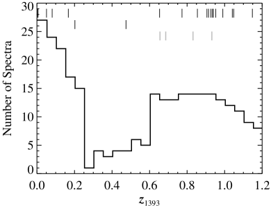
Figure 1: Schematic of redshift coverage for the current survey. The number of spectra with coverage of the Si IV doublet is shown as a function of $z_{1393}$ (histogram). The STIS E140M spectra covered $z_{1393}\lesssim 0.21$. The STIS E230M spectra typically covered $0.6\lesssim z_{1393}<1.2$. The redshift range $0.21\lesssim z_{1393}\lesssim 0.6$ was covered by some E230M spectra as well as STIS medium-resolution gratings and GHRS spectra. The redshifts of the doublets detected with $W_{r}\geq 3\,\sigma_{W_{r}}$ in both lines are shown with the hashes across the top. The top and middle rows indicate the redshifts of the 18 unsaturated and two saturated doublets, respectively, in the definite group (G = 1). The bottom row shows the redshift of the four unsaturated “highly-likely” (G = 2) doublets.

$\begin{array}[]{c}\includegraphics[height=195.12767pt,angle={90}]{fig2a.ps}\\ \includegraphics[height=195.12767pt,angle={90}]{fig2b.ps}\end{array}$

Figure 2: Redshift path length $\Delta X(\log N(\mathrm{Si}^{+3}))$ and $\Delta X(W_{r}{}_{,\mathrm{1393}})$ as a function of Si IV 1393 column density (top) and rest equivalent width respectively (bottom). These estimates are based on Monte Carlo analysis and correspond to 95% completeness limits.

Table 1: Si IV CANDIDATES SUMMARY

(1)	(2)	(3)	(4)	(5)	(6)	(7)	(8)	(9)	(10)
$z_{1393}$	$\delta v_{\rm abs}$	$\lambda_{r}$	$\lambda_{l}$	$\lambda_{h}$	$W_{r}$	$\sigma_{W_{r}}$	$\log N$	$\sigma_{\log N}$	Flag
	(​$\,{\rm km\,s}^{-1}$)	(Å)	(Å)	(Å)	(​ mÅ)	(​ mÅ)
MRK335 ($z_{\rm em}=0.026$)
$-0.00001$	$\cdots$	1393.76	1393.40	1394.04	212	15	13.55	0.04	495
	$-6.9$	1402.77	1402.41	1403.06	129	15	13.54	0.05
$0.00643$	$\cdots$	1393.76	1402.41	1403.03	125	14	13.23	0.05	317
	$-7.3$	1402.77	1411.48	1412.10	$<32$	$\cdots$	$<13.15$	$\cdots$
$0.01078$	$\cdots$	1393.76	1408.67	1408.91	$<20$	$\cdots$	$<12.65$	$\cdots$	173
	$0.7$	1402.77	1417.78	1418.02	37	12	12.97	0.14
PG0117+213 ($z_{\rm em}=1.493$)
$0.63473$	$\cdots$	1393.76	2278.01	2278.98	622	70	$>13.84$	$\cdots$	258
	$10.0$	1402.77	2292.74	2293.72	$<83$	$\cdots$	$<13.59$	$\cdots$
$0.63639$	$\cdots$	1393.76	2280.25	2281.14	$<116$	$\cdots$	$<13.41$	$\cdots$	160
	$-0.5$	1402.77	2295.00	2295.90	240	41	$>13.72$	$\cdots$
$0.63962$	$\cdots$	1393.76	2284.12	2286.44	478	67	$>13.95$	$\cdots$	259
	$94.0$	1402.77	2298.89	2301.23	$<167$	$\cdots$	$<13.81$	$\cdots$
TONS210 ($z_{\rm em}=0.116$)
$-0.00070$	$\cdots$	1393.76	1392.56	1393.09	81	12	13.04	0.06	367
	$-4.4$	1402.77	1401.57	1402.10	$<25$	$\cdots$	$<12.77$	$\cdots$
$-0.00002$	$\cdots$	1393.76	1393.34	1394.13	272	14	13.63	0.03	431
	$7.8$	1402.77	1402.35	1403.15	110	17	13.47	0.06
$0.00129$	$\cdots$	1393.76	1395.39	1395.69	29	9	12.55	0.14	301
	$-8.0$	1402.77	1404.42	1404.72	$<26$	$\cdots$	$<12.79$	$\cdots$

Note. — Summary of Si IV doublet candidates by target and redshift of Si IV 1393. Upper limits are $2\sigma$ limits for both $W_{r}$ and $\log N$. The binary flag is described in Section 3.

(This table is available in a machine-readable form in the online journal. A portion is shown here for guidance regarding its form and content.)

3 Si IV Sample Selection

Absorption lines with observed equivalent width $W_{\rm obs}\geq 3\sigma_{W_{\rm obs}}$ were automatically detected in the spectra. Candidate Si IV doublets were identified based solely on the characteristic wavelength separation of the doublet ($\approx\!1940\,{\rm km\,s}^{-1}$). First, each $W_{\rm obs}\geq 3\sigma_{W_{\rm obs}}$ line was assumed to be Si IV 1393, and any automatically-detected line that was near the location of would-be Si IV 1402 was adopted as such. If no $W_{\rm obs}\geq 3\sigma_{W_{\rm obs}}$ line existed, an upper limit was set on $W_{\rm obs}$ from the spectrum. Second, any automatically-detected line not already tagged as Si IV 1393 or 1402 was assumed to be the latter, and an upper limit was set on $W_{\rm obs}{}_{,1393}$ from the spectrum (see Paper I, for details). A summary of all candidate Si IV doublets are given in Table 1.

Other common absorption lines (e.g., $\mathrm{Ly}\alpha$ and C IV) were associated with the candidate systems in a similar manner. For example, an automatically-detected absorption line would be identified as a candidate $\mathrm{Ly}\alpha$ line if it had observed wavelength $\lambda\approx\lambda_{\alpha}(1+z_{\rm cand})$, where $\lambda_{\alpha}$ is the rest wavelength of $\mathrm{Ly}\alpha$ and $z_{\rm cand}$ is the redshift of the candidate Si IV doublet. The FUSE spectra were useful in this step, since they covered the $\mathrm{Ly}\beta$ $\lambda 1025$, O VI, and C III $\lambda 977$ lines for $z\lesssim 0.1$ candidate systems. The presence of associated lines increased the confidence of our identifications.

Each candidate doublet was assigned a machine-generated, binary flag that scaled with the number of desired characteristics of a true Si IV doublet. The characteristics (flags) are as follows:

• $W_{r}{}_{,\mathrm{1393}}\geq 3\sigma_{W_{r},\mathrm{1393}}$;

• $W_{r}{}_{,\mathrm{1402}}\geq 3\sigma_{W_{r},\mathrm{1402}}$;

• the ratio $W_{r}{}_{,\mathrm{1393}}:W_{r}{}_{,\mathrm{1402}}$ is in the range of $1:1$ to $2:1$ plus/minus the propagated error of the ratio;

• the optical depth-weighted centroids of the Si IV lines have $|\delta v_{\rm abs}|\leq 10\,{\rm km\,s}^{-1}$;

• there exists a candidate $\mathrm{Ly}\alpha$ line with $W_{r}{}_{,\mathrm{\alpha}}\geq 3\sigma_{W_{r},\mathrm{\alpha}}$;

• the 1393 line is outside of the $\mathrm{Ly}\alpha$ forest

• and outside the $\mathrm{H}_{2}$ forest;

• the smoothed AOD per pixel of the doublet lines agree within $1\sigma$ for $\geq 68.3\%$ of the pixel; and

• there exists one or more candidate lines (not H I) associated with the candidate doublet and with $W_{r}\geq 3\sigma_{W_{r}}$.

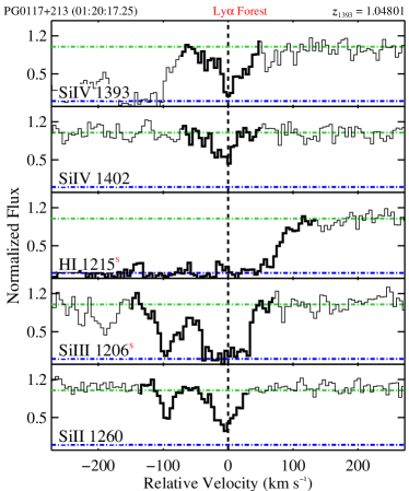
Figure 3: Velocity plots of 22 G = 1 Si IV systems. The regions of spectra around each absorption line are aligned in velocity space with respect to the rest wavelength of the transition and $z_{1393}$. Saturated transitions are indicated with the (red) ‘S’; any transition with column density detected at $<3\,\sigma$ are noted with a (red) ‘W.’ Systems with $z_{1393}<\lambda_{\alpha}(1+z_{\rm em})$ are labeled with a (red) “$\mathrm{Ly}\alpha$ Forest.” The regions used to measure $W_{r}$ and $\log N(\mathrm{Si}^{+3})$ are shown by the dark outline. The flux at zero and unity are shown with the dash-dot lines (blue and green, respectively); the vertical dashed line indicates $v=0\,{\rm km\,s}^{-1}$, corresponding to the optical depth-weighted velocity centroid of the Si IV 1393 transition. (The G = 1 velocity plots are available in their entirety in the online journal. One figure is shown here for guidance regarding the form and content.)

All candidates were visually inspected by at least one author, and the candidates with both lines detected at $W_{r}\geq 3\sigma_{W_{r}}$ were reviewed by two or more. We agreed upon 22 definite Si IV systems, which constitute the “G = 1” group (see Figure 3). Of these, 20 have both doublet lines detected with rest equivalent width $W_{r}\geq 3\sigma_{W_{r}}$ and constitute the group on which we based our conclusions. The G = 1 sample has a median redshift $\langle z\rangle=0.906$, $\log N(\mathrm{Si}^{+3})>12.9$, and $W_{r}{}_{,\mathrm{1393}}\geq 66\,\mbox{m\AA}$.

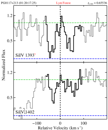
Figure 4: Velocity plots of six G = 2 Si IV systems. (See Figure 3 for description of velocity plot.) (The G = 2 velocity plots are available in their entirety in the online journal. One figure is shown here for guidance regarding the form and content.)

We also defined a small, “highly-likely” (G = 2) sample of six systems (see Figure 4). These doublets are typically found in regions with low S/N and/or do not have other lines associated with them, which would increase the confidence of our identification. The four of these with both lines detected at $\geq 3\sigma_{W_{r}}$ were combined with the G = 1 sample for some analyses and identified in tables and figures as G = 1+2. Details of all (G = 1+2) absorption systems are given in Table 2. The properties of the all Si IV doublets are summarized in Table 3.

All doublets are more than $1000\,{\rm km\,s}^{-1}$ outside of the Galaxy and $3000\,{\rm km\,s}^{-1}$ blue-ward of the background quasar. There were no Si IV absorbers without associated $\mathrm{Ly}\alpha$ absorption, when the spectral coverage existed to detect $\mathrm{Ly}\alpha$. We combined Si IV doublets into one absorption system when their optical depth-weighted centroids had $\delta v_{\rm abs}<250\,{\rm km\,s}^{-1}$.

The observed absorber line density is the sum of the number of absorbers, each weighted by the path length sensitive to their $N(\mathrm{Si}^{+3})$ or $W_{r}{}_{,\mathrm{1393}}$. For the G = 1 sample, $\mathrm{d}\mathcal{N}_{\mathrm{Si\,IV}}/\mathrm{d}X=1.4^{+0.4}_{-0.3}$ ($\mathrm{d}\mathcal{N}_{\mathrm{Si\,IV}}/\mathrm{d}z=2.7^{+0.7}_{-0.6}$) for $\log N(\mathrm{Si}^{+3})>12.9$.

As in Paper I, we conducted Monte Carlo simulations to measure the rate that pairs of $z\lesssim 1.5$ H I Lyman forest lines satisfy the characteristics of Si IV doublets and were potentially included in our sample as doublets. The contamination rate of forest lines masquerading as Si IV was small, less than 5% of $\mathrm{d}\mathcal{N}_{\mathrm{Si\,IV}}/\mathrm{d}X$ or an expected $1^{+2}_{-1}$ false doublet. If any doublet in our sample were false, it would be one without other associated absorption lines. There are four such doublets, all in the G = 2 sample. Our expectation that forest lines could mimic Si IV doublets drove us to define the “highly-likely” G = 2 group. Though we provide the results for analyses of the G = 1+2 sample, we only discuss the results from the G = 1 sample and base our conclusions on that; so we concern ourselves no further with the effects of the H I Lyman forest contamination.

3.1 Comparison with Previous Studies

There have been three recent surveys for Si IV systems at $z\lesssim 1$ using at least some of the HST spectra analyzed here: Milutinović et al. (2007); Danforth & Shull (2008), and Paper I. Here we briefly compare our blind doublet search results with these other studies. In the first two, they identified $\mathrm{Ly}\alpha$ lines first and then sought associated transitions

Milutinović et al. (2007) identified 17 Si IV doublets in the eight STIS E230M spectra that they surveyed. We independently identified 13 of those absorbers. The remaining four doublets were explicitly listed as questionable by these authors. We identified the G = 2, $z_{1393}=0.65536$ absorber in the PG0117+213 spectrum, one of the eight surveyed by Milutinović et al. (2007), though they did not detect it. Since only the doublet was detected, they would not have found it with their $\mathrm{Ly}\alpha$-targeted search.

Danforth & Shull (2008) surveyed all of the STIS E140M spectra for many transitions, including Si IV. They did not require that both doublet lines be detected with $W_{r}\geq 3\sigma_{W_{r}}$. They found 20 Si IV doublets for a line density $\mathrm{d}\mathcal{N}_{\mathrm{Si\,IV}}/\mathrm{d}X=5^{+2}_{-1}$ for $W_{r}\geq 30\,\mbox{m\AA}$.

In contrast, we found seven Si IV absorbers in the E140M spectra. There were two (G = 1) doublets that we identified in our Si IV-targeted survey but Danforth & Shull (2008) did not find: the $z_{1393}=0.00572$ doublet in QSO–123050+011522 and the $z_{1393}=0.13846$ one in PG1116+215. As mentioned in Paper I, Danforth & Shull (2008) missed the former doublet because the $\mathrm{Ly}\beta$ line in the FUSE spectra was suspect. The latter doublet has $W_{r}{}_{,\mathrm{1402}}<3\sigma_{W_{r},\mathrm{1402}}$, which might explain why they did not identify it.

Of their 20 systems, we agree with five and independently identified them in our Si IV-targeted survey. The remaining 15 doublets from Danforth & Shull (2008) were not included in our sample for at least one of the following reasons: one or both lines detected were at $W_{r}<3\sigma_{W_{r}}$ (12 doublets); one line was blended with a Galactic line (1); it was a system intrinsic to the background quasar (1); and/or the doublet was observed in the 0th order of E140M (2), which was exclude in our reduction.

We recovered all Si IV doublets that we previously identified in Paper I because of the association with a C IV system. We also determined that the G = 1, $z_{1548}=0.24010$ C IV doublet from Paper I is actually O I $\lambda 1302$ and Si II $\lambda 1304$ associated with the G = 1, $z_{1548}=0.47436$ system, which corresponds to our G = 1 Si IV system with $z_{1393}=z_{1548}$.

Table 2: Si IV SYSTEMS SUMMARY

(1)	(2)	(3)	(4)	(5)	(6)	(7)	(8)	(9)	(10)	(11)
$z_{1393}$	$\delta v_{\rm abs}$	$\lambda_{r}$	$\lambda_{l}$	$\lambda_{h}$	$W_{r}$	$\sigma_{W_{r}}$	$\log N$	$\sigma_{\log N}$	G	Flag
	(​$\,{\rm km\,s}^{-1}$)	(Å)	(Å)	(Å)	(​ mÅ)	(​ mÅ)
PG0117+213 ($z_{\rm em}=1.493$)
0.65536	$\cdots$	1393.76	2306.70	2307.89	273	28	$>13.73$	$\cdots$	2	482
	$9.2$	1402.77	2321.62	2322.82	122	24	13.54	0.09
1.04801	$\cdots$	1393.76	2853.75	2854.89	194	18	13.54	0.07	1	471
	$-10.5$	1402.77	2872.21	2873.36	83	14	13.37	0.07
	$-111.3$	1215.67	2486.96	2490.84	1530	21	$>14.88$	$\cdots$
	$-27.2$	1206.50	2469.68	2471.49	446	19	$>13.67$	$\cdots$
	$-26.2$	1260.42	2580.19	2581.61	145	11	13.16	0.03
B0312–770 ($z_{\rm em}=0.223$)
0.20253	$\cdots$	1393.76	1674.90	1676.82	652	78	$>14.16$	$\cdots$	1	511
	$7.6$	1402.77	1685.73	1687.67	543	57	$>14.40$	$\cdots$
	$-15.0$	1215.67	1460.66	1463.09	1677	20	$>14.92$	$\cdots$
	$-7.3$	1025.72	1232.52	1234.29	1139	20	$>15.59$	$\cdots$
	$11.2$	977.02	1174.06	1175.78	912	67	$>14.44$	$\cdots$
	$51.6$	1031.93	1240.64	1241.62	496	17	$>14.94$	$\cdots$
	$58.2$	1037.62	1247.48	1248.47	310	14	14.87	0.02
	$21.7$	1206.50	1449.82	1451.60	763	19	$>13.94$	$\cdots$
	$61.5$	1238.82	1489.57	1490.45	137	7	13.86	0.02
	$62.1$	1242.80	1494.36	1495.24	94	9	13.99	0.04
	$39.1$	1260.42	1515.44	1516.45	490	12	$>13.92$	$\cdots$
PKS0405–123 ($z_{\rm em}=0.573$)
0.16712	$\cdots$	1393.76	1626.40	1626.95	117	15	13.24	0.06	1	499
	$5.4$	1402.77	1636.92	1637.47	103	23	13.49	0.10
	$-18.1$	1215.67	1417.80	1419.38	876	19	$>14.60$	$\cdots$
	$-0.9$	1025.72	1196.77	1197.50	444	20	$>15.19$	$\cdots$
	$-22.2$	977.02	1139.53	1140.73	500	22	$>14.26$	$\cdots$
	$12.1$	989.80	1154.85	1155.66	214	12	$>14.64$	$\cdots$
	$-30.1$	1031.93	1203.74	1204.67	391	24	$>14.77$	$\cdots$
	$-50.7$	1037.62	1210.37	1211.31	218	37	14.80	0.11
	$2.3$	1206.50	1407.81	1408.40	236	11	$>13.38$	$\cdots$
	$-6.4$	1238.82	1445.53	1446.12	108	15	13.81	0.06
	$-7.4$	1242.80	1450.17	1450.76	76	13	13.94	0.07
	$-3.3$	1260.42	1470.73	1471.28	148	12	$>13.28$	$\cdots$

Note. — Si IV systems by target and redshift of Si IV 1393. Upper limits are $2\sigma$ limits for both $W_{r}$ and $\log N$. The column densities were measured by the AODM, unless “COG” is indicated, in which case, the limit is from assuming $W_{r}$ results from the linear portion of the COG. The definite Si IV doublets are labeled group G = 1, while the “highly-likely” doublets are G = 2. The binary flag is described in Section 3.

(This table is available in a machine-readable form in the online journal. A portion is shown here for guidance regarding its form and content.)

Table 3: Si IV DOUBLET SUMMARY

(1)	(2)	(3)	(4)		(5)		(6)		(7)		(8)
Target	G	$z_{1393}$	$W_{r}{}_{,\mathrm{1393}}$		$W_{r}{}_{,\mathrm{1402}}$		$\log N{}_{1393}$		$\log N{}_{1402}$		$\log N(\mathrm{Si}^{+3})$
			( mÅ)		( mÅ)
PG0117+213	2	0.65536	$273$	$\,\pm\,28$	$122$	$\,\pm\,24$	$>13.73$		$13.54$	$\,\pm\,0.09$	$13.54$	$\,\pm\,0.09$
	1	1.04801	$194$	$\,\pm\,18$	$83$	$\,\pm\,14$	$13.54$	$\,\pm\,0.07$	$13.37$	$\,\pm\,0.07$	$13.43$	$\,\pm\,0.05$
B0312–770	1	0.20253	$652$	$\,\pm\,78$	$543$	$\,\pm\,57$	$>14.16$		$>14.40$		$>14.40$
PKS0405–123	1	0.16712	$117$	$\,\pm\,15$	$103$	$\,\pm\,23$	$13.24$	$\,\pm\,0.06$	$13.49$	$\,\pm\,0.10$	$13.27$	$\,\pm\,0.05$
PKS0454–22	1	0.47436	$635$	$\,\pm\,52$	$475$	$\,\pm\,56$	$>13.84$		$>14.02$		$>14.02$
	1	0.48331	$112$	$\,\pm\,37$	$<61$		$>13.09$		$<13.34$		$[13.09$	$,13.38]$
HE0515–4414	2	0.68625	$249$	$\,\pm\,18$	$68$	$\,\pm\,17$	$<13.71$		$13.36$	$\,\pm\,0.10$	$13.36$	$\,\pm\,0.10$
	1	0.94047	$233$	$\,\pm\,13$	$56$	$\,\pm\,11$	$<13.58$		$13.15$	$\,\pm\,0.08$	$13.15$	$\,\pm\,0.08$
	1	1.14760	$565$	$\,\pm\,22$	$343$	$\,\pm\,29$	$13.98$	$\,\pm\,0.03$	$13.98$	$\,\pm\,0.04$	$13.98$	$\,\pm\,0.02$
HS0810+2554	2	0.55455	$250$	$\,\pm\,54$	$<160$		$>13.44$		$<14.06$		$[13.44$	$,13.76]$
	2	0.83143	$262$	$\,\pm\,30$	$271$	$\,\pm\,31$	$13.67$	$\,\pm\,0.08$	$13.91$	$\,\pm\,0.06$	$13.77$	$\,\pm\,0.05$
MARK132	2	0.93166	$73$	$\,\pm\,12$	$86$	$\,\pm\,12$	$12.95$	$\,\pm\,0.07$	$<13.31$		$12.95$	$\,\pm\,0.07$
PG1116+215	1	0.13846	$34$	$\,\pm\,9$	$<18$		$12.68$	$\,\pm\,0.10$	$<12.64$		$12.68$	$\,\pm\,0.10$
PG1206+459	1	0.92690	$777$	$\,\pm\,19$	$402$	$\,\pm\,29$	$14.08$	$\,\pm\,0.01$	$14.06$	$\,\pm\,0.03$	$14.08$	$\,\pm\,0.01$
	1	0.93429	$143$	$\,\pm\,11$	$98$	$\,\pm\,11$	$>13.51$		$13.60$	$\,\pm\,0.06$	$13.60$	$\,\pm\,0.06$
PG1211+143	1	0.05118	$66$	$\,\pm\,4$	$44$	$\,\pm\,5$	$12.96$	$\,\pm\,0.03$	$13.04$	$\,\pm\,0.05$	$12.97$	$\,\pm\,0.03$
MRK205	1	0.00428	$122$	$\,\pm\,11$	$75$	$\,\pm\,13$	$13.25$	$\,\pm\,0.04$	$13.33$	$\,\pm\,0.07$	$13.27$	$\,\pm\,0.04$
QSO–123050+011522	1	0.00572	$66$	$\,\pm\,8$	$63$	$\,\pm\,9$	$12.96$	$\,\pm\,0.05$	$13.21$	$\,\pm\,0.06$	$13.02$	$\,\pm\,0.04$
PG1248+401	1	0.77305	$472$	$\,\pm\,19$	$348$	$\,\pm\,17$	$>14.01$		$14.06$	$\,\pm\,0.02$	$14.06$	$\,\pm\,0.02$
	1	0.85485	$211$	$\,\pm\,21$	$138$	$\,\pm\,31$	$13.49$	$\,\pm\,0.05$	$13.59$	$\,\pm\,0.10$	$13.50$	$\,\pm\,0.04$
PG1630+377	1	0.91432	$123$	$\,\pm\,15$	$98$	$\,\pm\,12$	$13.26$	$\,\pm\,0.06$	$13.47$	$\,\pm\,0.06$	$13.33$	$\,\pm\,0.04$
	1	0.95279	$202$	$\,\pm\,15$	$136$	$\,\pm\,21$	$13.49$	$\,\pm\,0.04$	$13.59$	$\,\pm\,0.07$	$13.51$	$\,\pm\,0.03$
PG1634+706	1	0.65351	$145$	$\,\pm\,11$	$71$	$\,\pm\,9$	$13.30$	$\,\pm\,0.04$	$13.25$	$\,\pm\,0.06$	$13.29$	$\,\pm\,0.03$
	2	0.81813	$<15$		$21$	$\,\pm\,7$	$<12.25$		$12.71$	$\,\pm\,0.13$	$12.71$	$\,\pm\,0.13$
	1	0.90560	$182$	$\,\pm\,4$	$32$	$\,\pm\,5$	$<13.68$		$12.92$	$\,\pm\,0.07$	$12.92$	$\,\pm\,0.07$
	1	0.99035	$240$	$\,\pm\,7$	$162$	$\,\pm\,6$	$13.73$	$\,\pm\,0.02$	$13.74$	$\,\pm\,0.02$	$13.74$	$\,\pm\,0.01$
	1	1.04106	$167$	$\,\pm\,5$	$96$	$\,\pm\,8$	$13.32$	$\,\pm\,0.02$	$13.35$	$\,\pm\,0.03$	$13.33$	$\,\pm\,0.01$
PHL1811	1	0.08094	$108$	$\,\pm\,7$	$74$	$\,\pm\,9$	$>13.44$		$13.45$	$\,\pm\,0.05$	$13.45$	$\,\pm\,0.05$

Note. — Summary of Si IV doublets by target and redshift of Si IV 1393. The definite Si IV doublets are labeled group G = 1, while the “highly-likely” doublets are G = 2. Upper limits are $2\sigma$ limits for both $W_{r}$ and $\log N$. The adopted column density for the Si IV doublets are listed in the last column (see Section 2).

4 Analysis

4.1 Frequency Distributions

Analogous to the luminosity function used in galaxy studies, observers define the column density frequency distribution $f(N(\mathrm{Si}^{+3}))$ to be the number $\Delta\mathcal{N}$ of Si IV doublets per column density interval $\Delta N(\mathrm{Si}^{+3})$ per path length $\Delta X$ (see Figure 5). With a maximum likelihood fitting algorithm, we fit a power law to $f(N(\mathrm{Si}^{+3}))$ as follows:

$$f(N(\mathrm{Si}^{+3}))=k\,\bigg{(}\frac{N(\mathrm{Si}^{+3})}{N_{\rm 0}}\bigg{)}^{\alpha_{N}}{\rm,}$$ (1)

where $k$ is the normalization with unit ​$\,{\rm cm}^{2}$; $N_{\rm 0}=10^{13.5}\,{\rm cm}^{-2}$; and $\alpha_{N}$ is the slope. We often refer to $k_{14}$, which is the normalization $k$ scaled up by a factor of $10^{14}$. The frequency distribution was fit over the range $\log N_{\rm\rm min}=12.84$ to $\log N_{\rm\rm max}=15$, with special treatment of the saturated absorbers ($\log N{{}_{\rm sat}}=14$) in the maximum likelihood analysis (see Paper I, ). Briefly, the number of doublets with $14\leq\log N(\mathrm{Si}^{+3})\leq 15$ (i.e., saturated) was a constraint in our likelihood function. The best-fit parameters were: $k_{14}=1.18^{+0.45}_{-0.36}\,{\rm cm}^{2}$ and $\alpha_{N}=-1.61^{+0.28}_{-0.31}$.

The fit parameters for $f(N(\mathrm{Si}^{+3}))$ and $f(W_{r}{}_{,\mathrm{1393}})$ (discussed below) are given in Table 4. We estimated the 68.3% confidence limits (c.l.) in the power-law normalization and slope by tracing a contour where $\delta\mathcal{L}\equiv\ln\mathcal{L}-\ln\mathcal{L}_{\rm max}=-1.15$ on the likelihood surface $\mathcal{L}$, which included $68.3\%$ of its area. Then, the 68.3% c.l. (what we will loosely refer to as “1-$\sigma$ errors,” hereafter) were defined as the difference between the $k$ and $\alpha$ extrema on the contour and the $\mathcal{L}_{\rm max}$ values. Errors in quantities derived from the frequency distributions (e.g., the $\mathrm{Si}^{+3}$ mass density discussed below) are estimated in a similar fashion. The likelihood surface is not Gaussian, and the “2- and 3-$\sigma$ errors” are defined by $\delta\mathcal{L}=-3.15$ (95.4% c.l.) and $-6.1$ (99.7% c.l.), respectively. Therefore, the larger confidence limits on the best-fit power-law parameters are, formally, as follows: $2\sigma_{k_{14}}=+0.79/-0.54\,{\rm cm}^{2}$; $2\sigma_{\alpha_{N}}=+0.45/-0.53$; $3\sigma_{k_{14}}=+1.18/-0.70\,{\rm cm}^{2}$; and $3\sigma_{\alpha_{N}}=+0.62/-0.76$.

There was no observed break in $f(N(\mathrm{Si}^{+3}))$, and no break has been observed at high redshift. There must be a break in order to limit the number and mass of Si IV absorbers to finite quantities.

We have measured a slope consistent with those from high-redshift studies, though potentially shallower. Songaila (1997) measured $\alpha_{N}=-1.8$ for $2.16\leq z\leq 3$ and $-2$ for $3\leq z\leq 3.54$. Songaila (2001) and Scannapieco et al. (2006) stated that $\alpha_{N}=-1.8$ matched their observed $f(N(\mathrm{Si}^{+3}))$ well, which covered $1.78\leq z\leq 5.29$ and $1.5\leq z\leq 3.1$, respectively. From their $\mathrm{Ly}\alpha$-targeted $z<0.4$ survey, Danforth & Shull (2008) measured $\alpha_{N}=-1.92\pm 0.17$ for a sample with different selection criteria and from a survey with different methodology.

The definition of the equivalent width frequency distribution $f(W_{r}{}_{,\mathrm{1393}})$ is similar to that of $f(N(\mathrm{Si}^{+3}))$, and it was also fit well with a power law, with $W_{r}{}_{,\mathrm{0}}=150\,\mbox{m\AA}$, $W_{r}{}_{,\mathrm{min}}=57\,\mbox{m\AA}$, and $W_{r}{}_{,\mathrm{max}}=796\,\mbox{m\AA}$. The $W_{r}$ limits reflect the extrema of the observed values, $\pm 1\sigma$. The best-fit values for $f(W_{r}{}_{,\mathrm{1393}})$ were: $k_{3}=3.48^{+1.41}_{-1.12}\,\mbox{m\AA}^{-1}$ and $\alpha_{W}=-1.28^{+0.47}_{-0.47}$. The $W_{r}$ $k_{3}$ is the normalization scaled up by a factor of $10^{3}$. The larger confidence limits on the best-fit power-law parameters for $f(W_{r}{}_{,\mathrm{1393}})$ are, formally, as follows: $2\sigma_{k_{3}}=+2.55/\!-\!1.73\,\mbox{m\AA}^{-1}$; $2\sigma_{\alpha_{W}}=+0.79/\!-\!0.80$; $3\sigma_{k_{3}}=+3.81/\!-\!2.21\,\mbox{m\AA}^{-1}$; and $3\sigma_{\alpha_{W}}=+1.10/\!-\!1.13$.

Table 4: Si IV FREQUENCY DISTRIBUTIONS SUMMARY

(1)	(2)	(3)	(4)	(5)	(6)	(7)	(8)	(9)	(10)	(11)	(12)
G	$\langle z\rangle$	$z_{l}$	$z_{h}$	$\mathcal{N}$	Limits	$\mathrm{d}\mathcal{N}_{\mathrm{Si\,IV}}/\mathrm{d}z$	$\mathrm{d}\mathcal{N}_{\mathrm{Si\,IV}}/\mathrm{d}X$	$\Omega_{\mathrm{Si}^{+3}}\times 10^{8}$	$k$	$\alpha$	$P_{\rm KS}$
Column Density
1	0.90560	0.00428	1.14760	20	(12.84, 15.00)	$2.7^{+1.1}_{-0.8}$	$1.2^{+0.5}_{-0.4}$	$3.71^{+2.82}_{-1.68}$	$1.18^{+0.45}_{-0.36}$	$-1.61^{+0.28}_{-0.31}$	0.526
	0.91432			18	(12.92, 14.40)	$2.4^{+0.4}_{-0.3}$	$1.4^{+0.2}_{-0.2}$	$>1.63$	$\cdots$	$\cdots$	$\cdots$
1+2	0.85485	0.00428	1.14760	24	(12.84, 15.00)	$3.1^{+1.1}_{-0.9}$	$1.5^{+0.5}_{-0.4}$	$4.13^{+2.81}_{-1.77}$	$1.43^{+0.48}_{-0.39}$	$-1.65^{+0.26}_{-0.28}$	0.400
	0.90560			22	(12.92, 14.40)	$2.9^{+0.4}_{-0.3}$	$1.7^{+0.2}_{-0.2}$	$>1.94$	$\cdots$	$\cdots$	$\cdots$
Equivalent Width
1	0.90560	0.00428	1.14760	20	$(57,\,796)$	$3.0^{+1.2}_{-0.9}$	$1.4^{+0.5}_{-0.4}$	$\cdots$	$3.48^{+1.41}_{-1.12}$	$-1.28^{+0.47}_{-0.47}$	0.533
					$(66,\,777)$	$2.2^{+0.3}_{-0.3}$	$1.3^{+0.2}_{-0.1}$	$\cdots$	$\cdots$	$\cdots$	$\cdots$
1+2	0.85485	0.00428	1.14760	24	$(57,\,796)$	$3.5^{+1.3}_{-1.0}$	$1.6^{+0.6}_{-0.5}$	$\cdots$	$4.21^{+1.53}_{-1.24}$	$-1.30^{+0.43}_{-0.44}$	0.563
					$(66,\,777)$	$2.6^{+0.3}_{-0.3}$	$1.5^{+0.2}_{-0.2}$	$\cdots$	$\cdots$	$\cdots$	$\cdots$

Note. — Parameters from the maximum likelihood analysis for $f(x)=k\,(x/x_{0})^{\alpha}$, where $x=N(\mathrm{Si}^{+3})$ (or $W_{r}{}_{,\mathrm{1393}}$) and $x_{0}$ is $N_{\rm 0}=10^{13.5}\,{\rm cm}^{-2}$ ($W_{r}{}_{,\mathrm{0}}=150\,\mbox{m\AA}$). For each G = 1 or 1+2 subsample, the first row summarizes the maximum likelihood analysis and the second row, the observed quantities. $\mathrm{d}\mathcal{N}_{\mathrm{Si\,IV}}/\mathrm{d}X$, listed in the first subsample row, is the integral of $f(N(\mathrm{Si}^{+3}))$ ($f(W_{r}{}_{,\mathrm{1393}})$) from $\log N(\mathrm{Si}^{+3})=13$ to infinity ($W_{r}{}_{,\mathrm{1393}}=50\,\mbox{m\AA}$ to $796\,\mbox{m\AA}$) with the best-fit $k$ and $\alpha$. Also in the first subsample row, the integrated $\mathrm{d}\mathcal{N}_{\mathrm{Si\,IV}}/\mathrm{d}z\equiv\mathrm{d}\mathcal{N}_{\mathrm{Si\,IV}}/\mathrm{d}X\cdot\mathrm{d}X/\mathrm{d}z$, where the latter term is evaluated at $\langle z\rangle$. The observed $\mathrm{d}\mathcal{N}_{\mathrm{Si\,IV}}/\mathrm{d}z$ and $\mathrm{d}\mathcal{N}_{\mathrm{Si\,IV}}/\mathrm{d}X$ are from the sum of the total number of doublets, weighted by the path length available to detect the doublet, based on its $N(\mathrm{Si}^{+3})$ or $W_{r}{}_{,\mathrm{1393}}$. $\Omega_{\mathrm{Si}^{+3}}$, listed in the first subsample row in the column density section, is the integral of $f(N(\mathrm{Si}^{+3}))\cdot N(\mathrm{Si}^{+3})$ from $13\leq\log N(\mathrm{Si}^{+3})\leq 15$ with the best-fit $k$ and $\alpha$. The observed $\Omega_{\mathrm{Si}^{+3}}$ were from the sum of the unsaturated doublets, as given by $\mathcal{N}$. $P_{\rm KS}$ is the significance of the one-sided Kolmogorov-Smirnov statistic of the best-fit power law.

$\begin{array}[]{c}\includegraphics[height=195.12767pt,angle={90}]{fig5a.ps}\\ \includegraphics[height=195.12767pt,angle={90}]{fig5b.ps}\end{array}$

Figure 5: Column density (top) and rest equivalent width (bottom) frequency distributions for G = 1 and 1+2 samples (black and gray, respectively). The best-fit power laws, from the maximum likelihood analysis, are the dashed lines, with slope $\alpha$ and normalization $k_{14}$ as given. The column density saturation limit is indicated by the vertical, dotted line (top).

4.2 Si IV Absorber Line Density

We measured the observed Si IV line density by the sum of the number of absorbers, each weighted by the path length sensitive to their $N(\mathrm{Si}^{+3})$ or $W_{r}{}_{,\mathrm{1393}}$ (see Figure 2). For the G = 1 sample, $\mathrm{d}\mathcal{N}_{\mathrm{Si\,IV}}/\mathrm{d}X=1.4^{+0.4}_{-0.3}$ ($\mathrm{d}\mathcal{N}_{\mathrm{Si\,IV}}/\mathrm{d}z=2.4^{+0.7}_{-0.5}$) for $\log N(\mathrm{Si}^{+3})\geq 12.9$.

Since $f(N(\mathrm{Si}^{+3}))$ is modeled well by a power law, we can integrate Equation 1 to estimate the Si IV absorber line density $\mathrm{d}\mathcal{N}_{\mathrm{Si\,IV}}/\mathrm{d}X$ for a given column density limit $N_{\rm\rm lim}$:

$$\frac{\displaystyle\mathrm{d}\mathcal{N}_{\mathrm{Si\,IV}}}{\displaystyle\mathrm{d}X}(N(\mathrm{Si}^{+3})\geq N_{\rm\rm lim})=-\frac{k}{1+\alpha_{N}}\frac{N_{\rm\rm lim}^{1+\alpha_{N}}}{N_{\rm 0}^{\alpha_{N}}}{\rm.}$$ (2)

This is useful for comparing to high-redshift studies, which typically do not match our observational limits. In Figure 6, we show $\mathrm{d}\mathcal{N}_{\mathrm{Si\,IV}}/\mathrm{d}X$ as a function of $z_{1393}$ for $N_{\rm\rm lim}=10^{13}\,{\rm cm}^{-2}$.

The Si IV line density does not increase significantly from $z\approx 3\rightarrow 0$. Our integrated, $z\lesssim 1$ $\mathrm{d}\mathcal{N}_{\mathrm{Si\,IV}}/\mathrm{d}X=1.2^{+0.5}_{-0.4}$ ($\log N_{\rm\rm lim}=13$) is consistent within $1\sigma$ of the $\langle z\rangle=1.9$ value from Scannapieco et al. (2006) and $2\sigma$ of their $\langle z\rangle=2.7$ one. The formal errors on the integrated $\mathrm{d}\mathcal{N}_{\mathrm{Si\,IV}}/\mathrm{d}X$ are $2\sigma_{\mathrm{d}\mathcal{N}/\mathrm{d}X}=+1.3/\!-\!0.6$ and $3\sigma_{\mathrm{d}\mathcal{N}/\mathrm{d}X}=+1.2/\!-\!0.8$, derived from the $\alpha_{N}$ and $k_{14}$ errors discussed in Section 4.1. There is no evidence of evolution in $\mathrm{d}\mathcal{N}_{\mathrm{Si\,IV}}/\mathrm{d}X$ from $z=1\rightarrow 0$ (i.e., within our sample).

We estimated the high-redshift line densities and errors in the following manner. Scannapieco et al. (2006) published their $f(N(\mathrm{Si}^{+3}))$, from which we estimated the power-law normalization $k_{14}$ given the best-fit slope $\alpha_{N}$. We measured $f(N(\mathrm{Si}^{+3}))$ at several $N(\mathrm{Si}^{+3})$ and used the scatter as an estimate of the errors. We assumed $\alpha_{N}=-1.8$, as Scannapieco et al. (2006) did, and estimated $k_{14}=1.3\pm 0.9\,{\rm cm}^{2}$ for $\langle z\rangle=1.9$ and $k_{14}=0.5\pm 0.1\,{\rm cm}^{2}$ for $\langle z\rangle=2.7$.

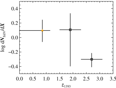
Figure 6: Redshift evolution of $\mathrm{d}\mathcal{N}_{\mathrm{Si\,IV}}/\mathrm{d}X$. The line density of Si IV absorbers has not increased significantly since $z\approx 3$. The (orange) stars are our $z\lesssim 1$ integrated values for $N(\mathrm{Si}^{+3})\geq 10^{13}\,{\rm cm}^{-2}$. The high-redshift values are integrated $\mathrm{d}\mathcal{N}_{\mathrm{Si\,IV}}/\mathrm{d}X$, with the slope and normalization estimated from the $f(N(\mathrm{Si}^{+3}))$ published in Scannapieco et al. (2006, black squares).

4.3 $\mathrm{Si}^{+3}$ Mass Density

The $\mathrm{Si}^{+3}$ mass density has been measured by several $1.5<z\lesssim 5.5$ studies (Songaila, 1997, 2001, 2005; Scannapieco et al., 2006). Typically, they measured the mass density, relative to the critical density $\rho_{c,0}$, by summing the detected absorbers (Lanzetta et al., 1991):

$$\Omega_{\mathrm{Si}^{+3}}=\frac{H_{0}\,\mathrm{m}_{\rm C}}{c\,\rho_{c,0}}\sum_{\mathcal{N}}\frac{N(\mathrm{Si}^{+3})}{\Delta X(N(\mathrm{Si}^{+3}))}{\rm,}$$ (3)

where the Hubble constant is $H_{0}=70\,{\rm km\,s}^{-1}\,\mathrm{Mpc}^{-1}$; the mass of a silicon atom is $\mathrm{m}_{\rm Si}=5\times 10^{-23}\,$g; $c$ is the speed of light; and $\rho_{c,0}=9.26\times 10^{-30}\,{\rm g}\,{\rm cm}^{-3}$. The summed $\Omega_{\mathrm{Si}^{+3}}$ approximates the mass density in all absorbers with column densities within the observed $N(\mathrm{Si}^{+3})$ range, which is $12\lesssim\log N(\mathrm{Si}^{+3})\lesssim 15$ for the high-redshift studies.

Since we measured column densities with the AODM, we only have lower limits on $N(\mathrm{Si}^{+3})$ for the strong, saturated doublets, which dominate $\Omega_{\mathrm{Si}^{+3}}$. Thus, summing the column densities only resulted in a lower limit $\Omega_{\mathrm{Si}^{+3}}\geq 1.55\times 10^{-8}$ for the 16 unsaturated G = 1 doublets with $\log N(\mathrm{Si}^{+3})\geq 13$. We exclude the two saturated doublets since they might have $\log N(\mathrm{Si}^{+3})>15$, which is the upper limit we have chosen for comparing $\Omega_{\mathrm{Si}^{+3}}$. Including the two saturated doublets, results in the summed $\Omega_{\mathrm{Si}^{+3}}>2.3\times 10^{-8}$ for the 18 G = 1 doublets with $\log N(\mathrm{Si}^{+3})\geq 13$.

In order to compare with the high-redshift studies, we assumed the power-law formalism for $f(N(\mathrm{Si}^{+3}))$ and integrated the column density-“weighted” $f(N(\mathrm{Si}^{+3}))$ (i.e., its first moment):

$$\Omega_{\mathrm{Si}^{+3}}=\frac{H_{0}\,\mathrm{m}_{\rm C}}{c\,\rho_{c,0}}\frac{k}{2+\alpha_{N}}\bigg{(}\frac{N_{\rm\rm max}^{2+\alpha_{N}}-N_{\rm\rm min}^{2+\alpha_{N}}}{N_{\rm 0}^{\alpha_{N}}}\bigg{)}{\rm.}$$ (4)

From the best-fit values for the G = 1 $f(N(\mathrm{Si}^{+3}))$, $\Omega_{\mathrm{Si}^{+3}}=(3.71^{+2.82}_{-1.68})\times 10^{-8}$ for $\log N_{\rm\rm min}=13$ and $\log N_{\rm\rm max}=15$. Since there has been no observed break in $f(N(\mathrm{Si}^{+3}))$, the column density limits are crucial to defining a finite $\Omega_{\mathrm{Si}^{+3}}$ and comparing between surveys.

The formal errors on the integrated $\Omega_{\mathrm{Si}^{+3}}$ are $2\sigma_{\Omega}=+5.54/\!-\!2.36$ and $3\sigma_{\Omega}=+8.99/\!-\!2.81$. derived from the $\alpha_{N}$ and $k_{14}$ errors discussed in Section 4.1.

We plot the evolution of $\Omega_{\mathrm{Si}^{+3}}$ as a function of the age of the Universe $t_{\rm age}$ in Figure 7. The median of the $2\leq z\leq 4.5$ studies (Songaila, 2001; Scannapieco et al., 2006, whose values have been adjusted to match our $N(\mathrm{Si}^{+3})$ limits and cosmology, see Paper I) is $\langle\Omega_{\mathrm{Si}^{+3}}\rangle^{2\leq z\leq 4.5}=(0.77^{+0.31}_{-0.21})\times 10^{-8}$, which is shown by the (blue) lines in Figure 7 (left). We have detected, with $>\!99.8\%$ confidence, an increase in $\Omega_{\mathrm{Si}^{+3}}$ from high-to-low redshift. The $z\lesssim 1$ is a factor of $4.8^{+3.0}_{-1.9}$ higher than the $2\leq z\leq 4.5$ median.

The confidence limits on the median high-redshift value and the increase in $\Omega_{\mathrm{Si}^{+3}}$ were estimated based on Monte Carlo sampling of the distributions. First, we drew $10^{6}$ realizations of the high-redshift data sets $\Omega_{\rm MC}^{2\leq z\leq 4.5}$, assuming they had log-normal errors. Then, we measured the median of each set: $\langle\Omega_{\rm MC}^{2\leq z\leq 4.5}\rangle_{i}$. The median $\mathrm{Si}^{+3}$ mass density quoted above ($\langle\Omega_{\mathrm{Si}^{+3}}\rangle^{2\leq z\leq 4.5}$) was the median of these ($10^{6}$) $\langle\Omega_{\rm MC}^{2\leq z\leq 4.5}\rangle_{i}$ values.

To Monte Carlo sample our $z\lesssim 1$ measurement, we used the likelihood surface discussed in Section 4.1 and the Metropolis-Hastings algorithm to appropriately sample the $k$-$\alpha_{N}$ parameter space $10^{6}$ times. For each of these random pairs, we computed the integrated $\mathrm{Si}^{+3}$ mass density (see Equation 4), resulting in a low-redshift Monte Carlo sample: $\Omega_{\rm MC}^{z\lesssim 1}$. The median of this distribution was: $\langle\Omega_{\mathrm{Si}^{+3}}\rangle^{z\lesssim 1}=(3.70^{+1.68}_{-1.19})\times 10^{-8}$. The ratio of the low- to high-redshift Monte Carlo samples (i.e., $\langle\Omega_{\rm MC}^{2\leq z\leq 4.5}\rangle_{i}/\Omega_{{\rm MC},i}^{z\lesssim 1}$) is a distribution where the median is $4.8^{+3.0}_{-1.9}$ and the ratio is greater than unity at the 99.8% c.l.

A least-squares minimization of a linear model to $\Omega_{\mathrm{Si}^{+3}}$ over $t_{\rm age}$ for the $2<z<5.5$ observations (Songaila, 2001; Scannapieco et al., 2006) and our $z\lesssim 1$ value yielded: $\mathrm{d}\Omega_{\mathrm{Si}^{+3}}/\mathrm{d}t_{\rm age}=(0.61\pm 0.23)\times 10^{-8}\,{\rm Gyr}$, as shown by the (red) lines in Figure 7 (right). This toy-model slope agrees well ($<\!2\sigma$) with $\mathrm{d}\Omega_{\mathrm{C}^{+3}}/\mathrm{d}t_{\rm age}=(0.42\pm 0.2)\times 10^{-8}\,{\rm Gyr}$ from Paper I for the equivalent redshift sample but for C IV absorbers, and D’Odorico et al. (2010) detected a smooth increase in $\Omega_{\mathrm{C}^{+3}}$ from $z=2.5\rightarrow 1.5$, which reaches the $z<1$ $\Omega_{\mathrm{C}^{+3}}$ measured in Paper I. A linear fit to only the $2\leq z<5.5$ observations indicated no temporal evolution in $\Omega_{\mathrm{Si}^{+3}}$ (i.e., $\mathrm{d}\Omega_{\mathrm{Si}^{+3}}/\mathrm{d}t_{\rm age}=(0.10\pm 0.56)\times 10^{-8}\,{\rm Gyr}$).

Modeling $\Omega_{\mathrm{Si}^{+3}}$ as evolving linearly with time was not a physically motivated exercise but one method to evaluate whether our $\Omega_{\mathrm{Si}^{+3}}$ indicated a significant increase compared to the high-redshift observations. Since the inclusion of our $z\lesssim 1$ value resulted in a statistically significant rate of increase for $\Omega_{\mathrm{Si}^{+3}}$, we likely have detected a true increase of the $\mathrm{Si}^{+3}$ mass density at low redshift, though proof must await a larger $z\lesssim 1$ survey.

Our results indicate that any increase in $\Omega_{\mathrm{Si}^{+3}}$ at $z\lesssim 1$ is likely due to an increase in the number of high-column density absorbers (i.e., shallower $\alpha_{N}$ compared to high redshift), since $\mathrm{d}\mathcal{N}_{\mathrm{Si\,IV}}/\mathrm{d}X$ is nearly constant from $z\approx 3\rightarrow 0$. In general, the $\mathrm{Si}^{+3}$ mass density is dominated by the high-column density absorbers, so even a small increase in their frequency will significantly change $\Omega_{\mathrm{Si}^{+3}}$.

$\begin{array}[]{cc}\includegraphics[height=203.80193pt,angle={90}]{fig7a.ps}&\includegraphics[height=203.80193pt,angle={90}]{fig7b.ps}\end{array}$

Figure 7: Time evolution of $\mathrm{Si}^{+3}$ mass density relative to the critical density. The integrated $\Omega_{\mathrm{Si}^{+3}}$, for $13\leq\log N(\mathrm{Si}^{+3})\leq 15$ for the G = 1 sample, is the (orange) star. The value from Danforth & Shull (2008) is the (green) triangle and is not an independent measurement of $\Omega_{\mathrm{Si}^{+3}}$. We compared our $z\lesssim 1$ measurement only to those from Songaila (2001, black crosses) and Scannapieco et al. (2006, black, open square). The median, and its “errors” (see Section 4.3), of the $2\leq z\leq 4.5$ values are shown on the left with the (blue) solid and dashed lines, respectively. The simple linear fit to $\Omega_{\mathrm{Si}^{+3}}$ over $t_{\rm age}$ is shown on the right by the (red) solid line, where the dashed lines are the 1-$\sigma$ range of the fit. For reference, we also show the values from Songaila (1997, gray circles) and Songaila (2005, gray, filled squares); the latter of which uses a pixel-optical depth method to measure $\Omega_{\mathrm{Si}^{+3}}$.

4.4 $N(\mathrm{Si}^{+3})/N(\mathrm{C}^{+3})$

As mentioned previously, the ionic ratio $N(\mathrm{Si}^{+3})/N(\mathrm{C}^{+3})$ has been used to study the shape and/or evolution of the UVB. In order to construct a complete sample of systems with coverage of both doublets, we measured the upper limit for $N(\mathrm{C}^{+3})$ (or $N(\mathrm{Si}^{+3})$) when the doublet was not detected in association with the targeted Si IV (or C IV, from Paper I) doublet but the spectral coverage existed. Due to how the S/N changed throughout any spectrum, a Si IV-targeted survey was not sufficient to define a complete C IV sample and visa versa. Ultimately, there were 12 detections and 12 lower limits for $z<1$ $N(\mathrm{Si}^{+3})/N(\mathrm{C}^{+3})$, with $\log N(\mathrm{Si}^{+3})>11.9$ and $\log N(\mathrm{C}^{+3})>13.37$.

In Figure 8, we compare our $N(\mathrm{Si}^{+3})/N(\mathrm{C}^{+3})$ sample with that from Boksenberg et al. (2003). We reproduced their Figure 16 (bottom panel) by summing the column densities of all components per system as given in their Tables 2–10. If there were components with upper limits for column densities, we set the total system column density to an upper limit if the components with upper limits were more than 30% of the total. If there were components with lower limits for column densities, we set the total column density to a lower limit. There was no case when these criteria conflicted. For the high-redshift sample, there were 39 detections and one upper limit for $N(\mathrm{Si}^{+3})/N(\mathrm{C}^{+3})$, for doublets with the observed low-redshift column density limits.

Since both high- and low-redshift samples contained at least one upper limit, we used survival analysis to enable those limits to contribute statistically. We used the Astronomy SURVival Analysis package (ASURV Rev. 1.3, last described in Lavalley et al., 1992) to compare the two $N(\mathrm{Si}^{+3})/N(\mathrm{C}^{+3})$ data sets. First, we tested whether the low-redshift $N(\mathrm{Si}^{+3})/N(\mathrm{C}^{+3})$ distribution shared the same parent population as the high-redshift ratios. From several univariate ASURV statistics, we conclude that the two populations are statistically similar (i.e., the null hypothesis cannot be ruled out with high confidence).

Next we measured the median ratio of the parent population with the Kaplan-Meier estimator. The estimated median of the combined low- and high-redshift data sets was $\langle N(\mathrm{Si}^{+3})/N(\mathrm{C}^{+3})\rangle=0.16$, and the 25th and 75th percentiles were 0.09 and 0.26, respectively.

Though the estimated means of the high- and low-redshift samples indicated that there should be no evolution of the ratio with redshift, we checked for a correlation. Once again, the null hypothesis (i.e., that there is no correlation) cannot be ruled out with high confidence.

$\begin{array}[]{cc}\includegraphics[height=203.80193pt,angle={90}]{fig8a.ps}&\includegraphics[height=203.80193pt,angle={90}]{fig8b.ps}\end{array}$

Figure 8: Ionic ratio $N(\mathrm{Si}^{+3})/N(\mathrm{C}^{+3})$ as a function of $N(\mathrm{C}^{+3})$ (left) and $z_{1393}$ (right). The $2\leq z_{1393}<4.5$ data (open circles) come from the total column densities per system from Boksenberg et al. (2003, Tables 2–10). The low-redshift data have $\log N(\mathrm{Si}^{+3})>11.9$ and $\log N(\mathrm{C}^{+3})>13.37$ (black, filled squares). High-redshift systems meeting these limits are the larger, black circles, while the rest of the sample are the smaller, gray circles. Survival analysis shows that the high- and low-redshift ratios are drawn from the same parent population and do not evolve significantly with redshift.

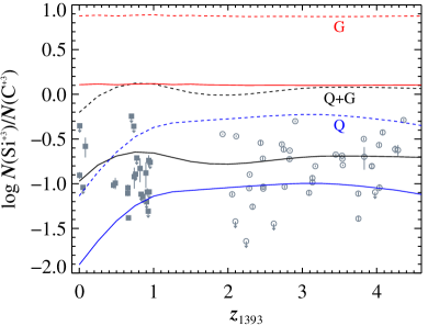
Figure 9: Predictions from simple photoionization models for $N(\mathrm{Si}^{+3})/N(\mathrm{C}^{+3})$ as a function of $z_{1393}$. All models could reproduce the observed lack of evolution in $N(\mathrm{Si}^{+3})/N(\mathrm{C}^{+3})$ with redshift and the overall magnitude of $N(\mathrm{Si}^{+3})/N(\mathrm{C}^{+3})$ through careful choice of the CLOUDY parameters (e.g., $\log U$, [Si/C]). For this plot, the ionization parameter is $\log U=-2$; the metallicity is $0.001\,Z_{\odot}$. The solid lines indicate models with solar relative abundances and the dashed lines, Si-enhanced (i.e., $[{\rm Si}/{\rm C}]=+0.77$). The gray, background points are the observations (black symbols from Figure 8, right), but the CLOUDY models were not fit to the observations.

4.5 Nature of Systems with Si IV and C IV Absorption

We concluded that there has been no evolution in $N(\mathrm{Si}^{+3})/N(\mathrm{C}^{+3})$ from $z=4.5\rightarrow 0$, based on our sample and that from Boksenberg et al. (2003). Next we explored what the lack of evolution means, and we began by disentangling the physics involved in the ratio $N(\mathrm{Si}^{+3})/N(\mathrm{C}^{+3})$:

$$\frac{N(\mathrm{Si}^{+3})}{N(\mathrm{C}^{+3})}=\Bigg{(}\frac{\displaystyle L_{\rm Si}}{\displaystyle L_{\rm C}}\Bigg{)}\Bigg{(}\frac{\displaystyle n_{\rm Si}}{\displaystyle n_{\rm C}}\Bigg{)}\Bigg{(}\frac{\displaystyle\chi^{\mathrm{Si}^{+3}}_{\rm Si}}{\displaystyle\chi^{\mathrm{C}^{+3}}_{\rm C}}\Bigg{)}{\rm,}$$ (5)

where $L_{\rm X}$ is the size of the cloud (enriched with X), along the line of sight; $n_{\rm X}$ is the volume density of element X; and $\chi^{\rm X^{\prime}}_{\rm X}$ is the fraction of X ionized into ion ${\rm X^{\prime}}$. The first term on the right-hand side is affected by the spatial distribution; the second, the metal abundances; and the third, the ionizing background.

The Universal trend is for structure to collapse and become denser with age in a $\Lambda$CDM Universe and for feedback processes to disperse and mix metals on varying scales. Therefore, more of the filamentary structure is enriched as the Universe ages; though feedback may preferentially enrich voids instead of filaments, as a result of the density difference (Kawata & Rauch, 2007). However, in our systems with both Si IV and C IV absorption, the absorption profiles trace each other quite well. There are no obvious system where $N(\mathrm{Si}^{+3})/N(\mathrm{C}^{+3})$ varies significantly between the components. Therefore, we infer $L_{\rm Si}\approx L_{\rm C}$.

We know that the metallicity of the Universe increases with age, but the relative abundance of silicon and carbon does not, necessarily, follow suit. Hence, the evolution in $n_{\rm Si}/n_{\rm C}$ is unclear.

We explored the effect of the ionizing background with a suite of simple photoionization models, in order to develop our understanding of the last term in Equation 5. We used the spectral synthesis program CLOUDY v08, as last described by Ferland et al. (1998). We modeled the medium as a plane-parallel slab, ionized by the Haardt & Madau (1996, updated in 2005) ultraviolet background, for quasar (Q), galaxy (G), and quasar+galaxy (Q+G) models. We set the number density of hydrogen $n_{\rm H}=0.1\,{\rm cm}^{-3}$, though our models were insensitive to this parameter in the optically-thin regime. We assumed a neutral column density $\log N_{\rm HI}=16$ and metallicity $Z=0.001\,Z_{\odot}$. We tested two cases: solar relative abundances and Si-enhanced; the increase in silicon was such that $[{\rm Si/C}]=+0.77$, as measured in Aguirre et al. (2004). We varied the ionization parameter $\log U=[-5,-4,-3,-2,-1]$, which is a dimensionless ratio of the flux of hydrogen-ionizing photons to $n_{\rm H}\cdot c$.

All models could reproduce the observed lack of evolution in the ionic ratios with redshift. In Figure 9, we show $N(\mathrm{Si}^{+3})/N(\mathrm{C}^{+3})$ as a function of redshift for the three UVB models, with solar relative abundances and Si-enhanced, and for $\log U=-2$. We did not fit the observations, but they are reproduced well by the solar relative abundance, Q+G model. More importantly, all UVB models could reproduce a shape consistent with the observed lack of evolution in $N(\mathrm{Si}^{+3})/N(\mathrm{C}^{+3})$, given the right choices of e.g., $\log U$, $\log N_{\rm HI}$, [Si/C]. The overall magnitude is nearly freely scalable by adjusting these parameters, because the observed sample of Si IV and C IV doublets are not drawn from a single type of cloud, as we modeled. Evidently, there is no need for a particularly soft UVB (i.e., model G) to reproduce the lack of redshift evolution in $N(\mathrm{Si}^{+3})/N(\mathrm{C}^{+3})$.

For there to be no evolution in $N(\mathrm{Si}^{+3})/N(\mathrm{C}^{+3})$ from $z=4.5\rightarrow 0$, the abundance, ionizing background, and structure of silicon- and carbon-enriched gas are constrained to be in “balance.” The observations indicate that these three processes evolved to maintain a constant ratio of $\langle N(\mathrm{Si}^{+3})/N(\mathrm{C}^{+3})\rangle=0.16$ for nearly 12 Gyr, for absorbers with $\log N(\mathrm{Si}^{+3})>11.9$ and $\log N(\mathrm{C}^{+3})>13.37$.

Disentangling the effect of the detailed physics (e.g., changing silicon and carbon abundances, variation in the physical properties of absorbing clouds) require cosmological hydrodynamic simulations that could resolve enrichment processes in galactic halos and the large-scale structure.

5 Summary

We conducted a blind survey for $z\lesssim 1$ Si IV doublets in the HST UV spectra of 49 quasars. We identified 22 definite Si IV systems (G = 1) and six “high-likely” ones (G = 2), and this represents the largest sample of low-redshift Si IV doublets prior to Servicing Mission 4. From a sample of 20 $z\lesssim 1$ Si IV doublets with both lines detected at $W_{r}\geq 3\sigma_{W_{r}}$, we measured a line density $\mathrm{d}\mathcal{N}_{\mathrm{Si\,IV}}/\mathrm{d}X=1.4^{+0.4}_{-0.3}$ for $\log N(\mathrm{Si}^{+3})>12.9$.

We constructed frequency distributions of the column densities $f(N(\mathrm{Si}^{+3}))$ and the rest equivalent widths $f(W_{r}{}_{,\mathrm{1393}})$. Both were approximated well by power laws. The best-fit power law to $f(N(\mathrm{Si}^{+3}))$ had slope $\alpha_{N}=-1.61^{+0.28}_{-0.31}$ and normalization $k=(1.18^{+0.45}_{-0.36})\times 10^{-14}\,{\rm cm}^{2}$. We compared the Si IV line density to high-redshift observations by integrating $f(N(\mathrm{Si}^{+3}))$, and $\mathrm{d}\mathcal{N}_{\mathrm{Si\,IV}}/\mathrm{d}X$ does not evolve significantly from $z\approx 3\rightarrow 0$.

From the first moment of $f(N(\mathrm{Si}^{+3}))$, we measured the $\mathrm{Si}^{+3}$ mass density relative to the critical density: $\Omega_{\mathrm{Si}^{+3}}=(3.71^{+2.82}_{-1.68})\times 10^{-8}$ for $13\leq\log N(\mathrm{Si}^{+3})\leq 15$. This value was estimated, with Monte Carlo sampling of the distributions, to be a factor of $4.8^{+3.0}_{-1.9}$ greater than the measurements from the $2\leq z\leq 4.5$ studies from Songaila (2001) and Scannapieco et al. (2006).

From a simple linear fit, we estimated the rate of increase in the $\mathrm{Si}^{+3}$ mass density over time to be $\mathrm{d}\Omega_{\mathrm{Si}^{+3}}/\mathrm{d}t_{\rm age}=(0.61\pm 0.23)\times 10^{-8}\,{\rm Gyr}$. Though a linear model is extremely simplistic and not physically motivated, it does lend support to the $z\lesssim 1$ $\Omega_{\mathrm{Si}^{+3}}$ being a true increase over the $1.5<z<5.5$ observations, which, when fit by themselves, result in no statistically significant temporal evolution.

Any increase in $\Omega_{\mathrm{Si}^{+3}}$ is probably driven by the increase in the number of high-column density absorbers (i.e., shallower $\alpha_{N}$), since $\mathrm{d}\mathcal{N}_{\mathrm{Si\,IV}}/\mathrm{d}X$ does not increase significantly from $z\approx 3\rightarrow 0$.

We also compared the ionic ratio $N(\mathrm{Si}^{+3})/N(\mathrm{C}^{+3})$ from the current study and Paper I with the high-redshift sample of Boksenberg et al. (2003). From survival analysis of the two populations, we concluded that the ionic ratios of the high- and low-redshift distributions are drawn from the same parent population, with median $\langle N(\mathrm{Si}^{+3})/N(\mathrm{C}^{+3})\rangle=0.16$. The lack of evolution in $N(\mathrm{Si}^{+3})/N(\mathrm{C}^{+3})$ from $z=4.5\rightarrow 0$ places constraints on the evolution of the metal production, feedback processes, and the ionizing background. These three processes evolve in some balanced fashion to have Si IV and C IV absorbers evolve in lock-step for the last $\approx\!12\,{\rm Gyr}$.

We explored the effect of the ionizing background on the (non)evolution of $N(\mathrm{Si}^{+3})/N(\mathrm{C}^{+3})$ with a suite of simple CLOUDY models. We varied the background by using the canonical Haardt & Madau (1996) quasar, galaxy, and quasar+galaxy models. All three backgrounds could result in relatively constant $N(\mathrm{Si}^{+3})/N(\mathrm{C}^{+3})$ over redshift, for models with the “right” choices of e.g., ionizing parameter, [Si/C]. Therefore, a soft UVB (i.e., model G) is not preferred.

In general, more observations—at low and high redshift—are needed to increase the statistical significance of the trends that are currently highly suggestive. We eagerly anticipate new low-redshift results from the HST Cosmic Origins Spectrograph (COS, Morse et al., 1998). Meanwhile, cosmological hydrodynamic simulations should be leveraged to understand how metal production and dispersal and the ionizing background interact to evolve Si IV and C IV absorbers in tandem.

References

- Aguirre et al. (2004) Aguirre, A., Schaye, J., Kim, T.-S., Theuns, T., Rauch, M., & Sargent, W. L. W. 2004, ApJ, 602, 38
- Bertschinger (1998) Bertschinger, E. 1998, ARA&A, 36, 599
- Boksenberg et al. (2003) Boksenberg, A., Sargent, W. L. W., & Rauch, M. 2003, ArXiv Astrophysics e-prints
- Bolton & Viel (2010) Bolton, J. S., & Viel, M. 2010, ArXiv e-prints
- Cooksey et al. (2008) Cooksey, K. L., Prochaska, J. X., Chen, H.-W., Mulchaey, J. S., & Weiner, B. J. 2008, ApJ, 676, 262
- Cooksey et al. (2010) Cooksey, K. L., Thom, C., Prochaska, J. X., & Chen, H. 2010, ApJ, 708, 868
- Danforth & Shull (2008) Danforth, C. W., & Shull, J. M. 2008, ApJ, 679, 194
- Davé & Oppenheimer (2007) Davé, R., & Oppenheimer, B. D. 2007, MNRAS, 374, 427
- D’Odorico et al. (2010) D’Odorico, V., Calura, F., Cristiani, S., & Viel, M. 2010, MNRAS, 401, 2715
- Feigelson & Nelson (1985) Feigelson, E. D., & Nelson, P. I. 1985, ApJ, 293, 192
- Ferland et al. (1998) Ferland, G. J., Korista, K. T., Verner, D. A., Ferguson, J. W., Kingdon, J. B., & Verner, E. M. 1998, PASP, 110, 761
- Haardt & Madau (1996) Haardt, F., & Madau, P. 1996, ApJ, 461, 20
- Isobe et al. (1986) Isobe, T., Feigelson, E. D., & Nelson, P. I. 1986, ApJ, 306, 490
- Kawata & Rauch (2007) Kawata, D., & Rauch, M. 2007, ApJ, 663, 38
- Kim et al. (2002) Kim, T., Cristiani, S., & D’Odorico, S. 2002, A&A, 383, 747
- Lanzetta et al. (1991) Lanzetta, K. M., McMahon, R. G., Wolfe, A. M., Turnshek, D. A., Hazard, C., & Lu, L. 1991, ApJS, 77, 1
- Lavalley et al. (1992) Lavalley, M. P., Isobe, T., & Feigelson, E. D. 1992, in Bulletin of the American Astronomical Society, Vol. 24, Bulletin of the American Astronomical Society, 839–840
- Madau & Haardt (2009) Madau, P., & Haardt, F. 2009, ApJ, 693, L100
- Milutinović et al. (2007) Milutinović, N., et al. 2007, MNRAS, 382, 1094
- Morse et al. (1998) Morse, J. A., et al. 1998, in Society of Photo-Optical Instrumentation Engineers (SPIE) Conference Series, Vol. 3356, Society of Photo-Optical Instrumentation Engineers (SPIE) Conference Series, ed. P. Y. Bely & J. B. Breckinridge, 361–368
- Oppenheimer & Davé (2008) Oppenheimer, B. D., & Davé, R. 2008, MNRAS, 387, 577
- Savage & Sembach (1991) Savage, B. D., & Sembach, K. R. 1991, ApJ, 379, 245
- Scannapieco et al. (2006) Scannapieco, E., Pichon, C., Aracil, B., Petitjean, P., Thacker, R. J., Pogosyan, D., Bergeron, J., & Couchman, H. M. P. 2006, MNRAS, 365, 615
- Simcoe et al. (2004) Simcoe, R. A., Sargent, W. L. W., & Rauch, M. 2004, ApJ, 606, 92
- Songaila (1997) Songaila, A. 1997, ApJ, 490, L1+
- Songaila (1998) —. 1998, AJ, 115, 2184
- Songaila (2001) —. 2001, ApJ, 561, L153
- Songaila (2005) —. 2005, AJ, 130, 1996
- Wiersma et al. (2009) Wiersma, R. P. C., Schaye, J., Theuns, T., Dalla Vecchia, C., & Tornatore, L. 2009, MNRAS, 399, 574