Leaders, Followers, and Community Detection

Abstract

Communities in social networks or graphs are sets of well-connected, overlapping vertices. The effectiveness of a community detection algorithm is determined by accuracy in finding the ground-truth communities and ability to scale with the size of the data. In this work, we provide three contributions. First, we show that a popular measure of accuracy known as the F1 score, which is between 0 and 1, with 1 being perfect detection, has an “information lower bound” is 0.5. We provide a trivial algorithm that produces communities with an F1 score of 0.5 for any graph! Somewhat surprisingly, we find that popular algorithms such as modularity optimization, BigClam and CESNA have F1 scores less than 0.5 for the popular IMDB graph. To rectify this, as the second contribution we propose a generative model for community formation, the sequential community graph, which is motivated by the formation of social networks. Third, motivated by our generative model, we propose the “leader-follower algorithm” (LFA). We prove that it recovers all communities for sequential community graphs by establishing a structural result that sequential community graphs are chordal. For a large number of popular social networks, it recovers communities with a much higher F1 score than other popular algorithms. For the IMDB graph, it obtains an F1 score of 0.81. We also propose a modification to the LFA called the fast leader-follower algorithm (FLFA) which in addition to being highly accurate, is also fast, with a scaling that is almost linear in the graph / network size.

I Introduction

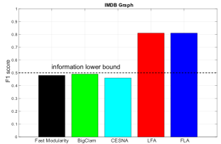
Figure 1: F1 score on IMDB graph for several community detection algorithms, including our leader-follower and fast leader-follower algorithms (LFA and FLFA). A lower bound of $0.5$ based on an algorithm that does not utilize any information is indicated by the dashed line.

Understanding community structure is an important and well studied problem in the analysis of social networks. Communities represent a latent structure that is manifested through densely connected vertices. For example, a latent social group such co-workers may show up as a set of people in a social network connected by a dense set of edges. While many community detection algorithms have been proposed (cf. fortunato2010community ), an important question is how to evaluate their performance. One approach is to compare the detected communities to a ground-truth set of communities if feasible. In this case, one needs to define some notion of distance between two sets of communities.

In yangcommunity the F1 score, which is based on concepts from information retrieval, is used to assess the accuracy of community detection methods. The score assigns a value between $0$ and $1$. It gives a higher value to communities which are closer to the ground-truth communities. The question is, what is a good F1 score? Clearly, 1 is an excellent score because it means perfect identification. But, for example, consider a popular IMDB graph for which we evaluate three excellent algorithms from the literature: modularity optimization newman2006modularity , CESNA yangcommunity and BigClam yang2013overlapping . Their respective F1 scores for the IMDB graph of $0.48,0.46$ and $0.49$ are shown in Figure 1. Are these scores good, okay or terrible?

Our contributions. To answer this question, as an important contribution we establish a non-trivial lower bound for the F1 score. Specifically, we show that there exists a simple algorithm that can produce communities with an F1 score of $0.5$ for any graph without accessing the graph structure. That is, $0.5$ is information lower bound on community detection. In that sense, for the IMDB graph mentioned above, the F1 scores of modularity optimization, CESNA and BigClam are simply terrible: based on the F1 score, these algorithms are unable to extract any meaningful information from the graph structure.

This clearly suggests that we need a better algorithm, at least for the type of community detection that graphs like IMDB require. To design such an algorithm, we need to understand how communities such as those in the IMDB network are formed. Towards that, we introduce a simple, but insightful generative model for community formation which we call the sequential community graph model. In this model, vertices (individuals) arrive sequentially and either join existing communities in the graph or form a new community. Unlike the models in yang2013overlapping and yangcommunity , our model is a combinatorial model and does not have any (hyper-)parameters.

The value of the model, in a sense, is in its ability to unearth communities hidden in a graph structure using an appropriate algorithm. We show that, for a graph generated by the sequential community model, there exists an extremely simple algorithm which we call the leader-follower algorithm (LFA), that can find all the communities successfully (see Theorem 3). The key property that we identify to establish this result is that all sequential community graphs are chordal graphs, and the LFA algorithm is effectively identifying the maximal cliques in this chordal graph. The LFA algorithm works for any graph and its running time is bounded by $O(|V|^{2}|E|)$ for a graph with vertex set $V$ and edge set $E$ (see Theorem 5).

While this running time is polynomial, it can be prohibitively expensive for very large graphs. To that end, we propose a natural heuristic that simplifies the LFA algorithm, which we call fast leader-follower algorithm (FLFA). It runs in time $O(|E|+|V|\log|V|)$ for graphs with vertex set $V$ and edge set $E$, i.e. FLFA is effectively linear in the input data size (see Theorem 4). We establish that the FLFA finds a specific subset of communities correctly for sequential community graphs (see Theorem 2).

The purpose of the sequential community graph model was to identify an algorithm that can perform well for graphs like the IMDB graph, as mentioned earlier. We evaluate the performance of our algorithms on the IMDB graph and find that both of them have F1 scores of 0.81, which is definitely better than the information lower bound of 0.5 (see Figure 1). We evaluate the algorithm’s performance for other datasets studied in the literature where ground truth communities are known. We find that for all such datasets, the LFA (and FLFA) outperform the representative known algorithms, namely, fast modularity optimization newman2006modularity and statistical inference based methods ( CESNA yangcommunity and BigClam yang2013overlapping ). We note that the FLFA runs orders of magnitude faster than all the other algorithms. The precise results are described in Section VI).

Related work. There are multiple approaches for community detection. Some are based on heuristics, such as modularity optimization newman2006modularity and k-clique percolation palla2005uncovering . More recently, there has been a lot of activity around developing statistical inference based algorithms for community detection by positing probabilistic generative model for communities. This includes the stochastic blockmodel and its variants airoldi2008mixed ; handcock2007model ; daudin2008mixture ; newman2016estimating ; karrer2011stochastic ; yang2013overlapping ; yangcommunity ; decelle2011asymptotic . One benefit of model based approaches is that they allow one to establish theoretical performance guarantees krzakala2013spectral ; hajek2016achieving ; mossel2015consistency ; abbe2016exact ; abbe2015recovering .

Many community detection methods can be difficult to implement exactly, but very often efficient approximations have been found. Modularity optimization is well known to be an NP-hard problem kar72 , but a very efficient procedure for modularity optimization is proposed in blondel2008fast . Statistical inference based methods can suffer in terms of scaling with data size due to the complexity of the inference task, but clever approaches have helped overcome such challenges, for example decelle2011asymptotic ; krzakala2013spectral ; yang2013overlapping ; yangcommunity

Organization. The remainder of the paper is organized as follows. Section II introduces the F1 score for community detection algorithms as well as our result on a non-trivial lower bound for it. Section III presents the sequential community graph model. Section IV presents the leader follower algorithm (LFA) and its efficient variant (FLFA). We establish their theoretical properties as well. We present an empirical evaluation of our algorithms in Section VI and conclude in Section VII.

II The Score Function

We are given an undirected graph $G=(V,E)$ where $V=\{v_{1},\dots,v_{n}\}$ represents vertices and $E\subset V\times V$ represents edges between them. We refer to $G$ as an observation graph because it represents all observed interactions between the vertices. The observation graph is generated through some unobserved process by a set of latent communities $\mathcal{C}=\left\{c_{1},c_{2},...,c_{m}\right\}$, where $c_{i}\subseteq V$ for $i=1,2,...,m$. The community detection problem is to use the observation graph $G$ to recover the latent communities $\mathcal{C}$.

To assess the accuracy of community detection algorithms, we define a score to compare sets of communities. For any two sets of communities $\mathcal{C}$ and $\mathcal{C}^{\prime}$ of an observation graph, we define their score as

$$d(\mathcal{C},\mathcal{C}^{\prime}) =\frac{1}{2}\left(s(\mathcal{C},\mathcal{C}^{\prime})+s(\mathcal{C}^{\prime},\mathcal{C})\right)$$ (1)

where we have defined $s(\mathcal{C},\mathcal{C}^{\prime})$ as

$$s(\mathcal{C},\mathcal{C}^{\prime}) ={\frac{1}{|\mathcal{C}|}\sum_{c\in\mathcal{C}}\max_{c^{\prime}\in\mathcal{C}^{\prime}}\delta(c,c^{\prime})}$$ (2)

and $\delta(c,c^{\prime})$ is a similarity measure between two communities. There are a variety of similarity measures we can choose, but we will follow the approach of yangcommunity and use the F1 score which is used commonly in binary classification. For two communities $c$ and $c^{\prime}$, we define the precision $p=|c\bigcap c^{\prime}|/|c^{\prime}|$ and the recall $r=|c\bigcap c^{\prime}|/|c|$. The F1 score is given by the harmonic mean of $p$ and $r$: $\delta(c,c^{\prime})=2pr/(p+r)$. For two identical community sets, the F1 score is one and the minimum value of the F1 score is zero for two disjoint communities.

The quantity $s(\mathcal{C},\mathcal{C}^{\prime})$ finds the best match in $\mathcal{C}^{\prime}$ for every community in $\mathcal{C}$. It then calculates the average similarity score of this matching. Note that multiple communities in $\mathcal{C}$ are allowed to match to the same community in $\mathcal{C}^{\prime}$ to allow for the possibility that communities in $\mathcal{C}$ are subsets of the same community in $\mathcal{C}^{\prime}$. The overall score, $d(\mathcal{C},\mathcal{C}^{\prime})$ is simply the average of $s(\mathcal{C},\mathcal{C}^{\prime})$ and $s(\mathcal{C}^{\prime},\mathcal{C})$. To see why our score needs both $s(\mathcal{C},\mathcal{C}^{\prime})$ and $s(\mathcal{C}^{\prime},\mathcal{C})$, consider the case where $\mathcal{C}=\{a\}$ and $\mathcal{C}^{\prime}=\{a,b,c,d,e,f\}$. If our score only accounted for $s(\mathcal{C},\mathcal{C}^{\prime})$, we would obtain a score of $1$, even though the communities are clearly quite different. The quantity $s(\mathcal{C}^{\prime},\mathcal{C})=1/5$. Hence, we need to account for the both $s(\mathcal{C},\mathcal{C}^{\prime})$ and $s(\mathcal{C}^{\prime},\mathcal{C})$ to obtain an informative score for two sets of communities.

To understand what constitutes a good value of this score, we consider the set of communities which is the power set of the vertices. The communities in this set are every possible subset of $V$. This is an extremely trivial community set and provides no information about community structure. We have the following result about the score of the power set communities and any arbitrary set of communities.

Lemma 1.

Let $\mathcal{C}$ be an arbitrary set of communities of a set of vertices $V$ and let the power set of $V$ be $\mathcal{P}$. Then

$$d(\mathcal{C},\mathcal{P})\geq 0.5.$$

This shows that the most uninformative community set will score at least 0.5. We will refer to this as the information lower bound. The output of a community detection algorithm must produce a score greater that 0.5 in order to be considered non-trivial. This is an important result because in previous works algorithms achieve scores below this threshold, showing that no informative community structure has been found yang2012community ; yangcommunity ; ruan2013efficient

Proof.

Every set in $\mathcal{C}$ matches exactly with one set in $\mathcal{P}$ and will have an F1 score of one. Therefore $s(\mathcal{C},\mathcal{P})=1$ which immediately leads to $d(\mathcal{C},\mathcal{P})\geq 0.5$. ∎

III Generating Communities:
Sequential Community Graphs

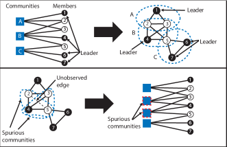
Figure 2: A latent community graph (top left) and its corresponding observation graph (top right). The leader vertices are colored black and the communities in the observation graph are circled with dashed lines. (bottom) Example of spurious communities created by an unobserved edge in the observation graph.

III.1 Latent Community Graphs

We assume that the observation graph $G$ is generated by an underlying latent or unobserved community structure $\mathcal{C}$. To make this more precise, let ${\mathcal{G}}=(V,{\mathcal{C}},{\mathcal{E}})$ represent the bipartite latent community graph, where one set of vertices is $V$ (the vertices we observe in $G$) and the other set is ${{\mathcal{C}}}=\{c_{1},\dots,c_{m}\}$ is the $m$ communities. The edges ${\mathcal{E}}\subset V\times{\mathcal{C}}$ are between these two sets, i.e. ${\mathcal{G}}$ is bipartite. The edges of ${\mathcal{E}}$ represent the membership of vertices of $V$ in communities of ${\mathcal{C}}$: $(i,c)\in{\mathcal{E}}$ if vertex $i$ belongs to community $c$. The observation graph $G=(V,E)$ is a projection of ${\mathcal{G}}$: $(i,j)\in E$ if and only if vertices $i,j\in V$ share one or more communities in ${\mathcal{G}}$, i.e. there exists $c\in{\mathcal{C}}$ such that $(i,c),(j,c)\in{\mathcal{E}}$. We illustrate these graphs in Figure 2.

One property of the latent bipartite community graph is that the resulting communities in the observation graph will be cliques. The latent bipartite community graph which explains the observation graph with the fewest number of communities will be such that each community is a maximal clique. Recall that a subset $c$ of vertices $V$ is called a clique if $\{(i,j):i\neq j\in c\}\subset E$; it is a maximal clique if there is no $c^{\prime}\subset V$ such that $c\subset c^{\prime}$ and $c^{\prime}$ is a clique as well. Note that for any given $G$, it is feasible to find a ${\mathcal{G}}$ so that $G$ becomes the corresponding projection of ${\mathcal{G}}$, but the communities are not guaranteed to be maximal cliques. Because such a set of communities may not be informative, we focus on finding communities which are maximal cliques. It is well known that the problem of finding maximal cliques in an arbitrary graph is computationally hard kar72 . The question of interest is are there prevalent social phenomenon generating latent community graphs for which finding communities in the observation graph is easy? To answer this question, we shall present the sequential community graph model next.

A few remarks are in order before we present the model. First, our problem formulation as well as the latent community graph has been considered before breiger1974duality ; simmel2010conflict ; feld1981focused ; yang2012community . Second, in practice there may be missing edges or noise in an observation graph. Statistical inference based models allow for these missing edges via a probabilistic mapping from the latent community graph to the observation graph yang2012community . In our situation, missing edges would cause true communities to no longer be cliques. For instance, if an edge is removed from a clique with $n$ vertices, then it becomes the union of two overlapping cliques each with $n-1$ vertices. Therefore, noise or missing edges in an observation graph will result in the creation of spurious community vertices in the corresponding latent community graph. We illustrate this in Figure 2. For the purposes of establishing theoretical results, we shall assume that $G$ is perfectly observed. However, as we shall see, our algorithms are robust to noisy observations.

III.2 Sequential Community Graphs

Here we present a generative model for latent community graphs which we call the sequential community graph model. This model should be treated as a social hypothesis applicable to a class of social scenarios. In particular, this model is relevant to settings where individuals enter a social graph by either joining existing communities or creating their own. We now present the model in detail.

Let ${\mathcal{G}}_{n}=(V_{n},{\mathcal{C}}_{n},{\mathcal{E}}_{n})$ denote a sequential community graph with $n$ observed vertices, i.e. $|V_{n}|=n$. This graph is generated sequentially as follows. Initially, $n=1$ and $V_{1}=\{v_{1}\}$, ${\mathcal{C}}_{1}=\{c_{1}\}$ and ${\mathcal{E}}_{1}=\{(1,c_{1})\}$. Given ${\mathcal{G}}_{i}$, ${\mathcal{G}}_{i+1}$ is generated by adding vertex $v_{i+1}$ to $V_{i}$, i.e. $V_{i+1}=V_{i}\cup\{v_{i+1}\}=\{v_{1},\dots,v_{i+1}\}$. For ${\mathcal{C}}_{i+1}$ and ${\mathcal{E}}_{i+1}$, one of the two choices listed below is exercised arbitrarily:

1. Choice 1. Choose a single community, $c\in{\mathcal{C}}_{i}$; add edge $(v_{i+1},c)$ to ${\mathcal{E}}_{i}$ to obtain ${\mathcal{E}}_{i+1}$ and set ${\mathcal{C}}_{i+1}={\mathcal{C}}_{i}$.

2. Choice 2. Add a new community vertex $c^{\prime}$ to ${\mathcal{C}}_{i}$ to obtain ${\mathcal{C}}_{i+1}$ and add a new edge $(v_{i+1},c^{\prime})$ to ${\mathcal{E}}_{i}$ to obtain ${\mathcal{E}}_{i+1}$. Then select any one other community vertex $c\in{\mathcal{C}}_{i}$. Let $V_{c}=\{v\in V:(v,c)\in{\mathcal{E}}_{i}\}$ be the neighbors of $c$ and select an arbitrary proper subset $V^{\prime}_{c}\subset V_{c}$ ($V^{\prime}_{c}$ can also be the empty set). Add edges $\{(v,c^{\prime}):v\in V^{\prime}_{c}\}$ to ${\mathcal{E}}_{i+1}$.

In a sequential community graph ${\mathcal{G}}_{n}$ there can be a maximum of $n$ community vertices because a new community vertex can only be generated by a new observation vertex. Also note that the construction of a sequential community graph is not unique. There can be multiple sequences of vertices that produce a given sequential community graph. We illustrate this with an example in Figure 3.

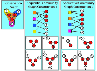
Figure 3: Illustration of two sequential community graph constructions (and the sequential construction of the corresponding observation graph) resulting in the same observation graph. In each construction the member vertices are listed in order of addition to the graph with the newest vertex at the bottom.

The sequential community graph model corresponds to social phenomena where new members join a social network by either joining an existing community or generating a new community from a subset of an existing community. Thus, new communities are only created when new members join the graph. This is not an unreasonable assumption. Consider for example the graph formed by the friends of an individual in an online social network. Communities are the mechanism by which people become friends with this individual. Either the friendship is formed from an existing community, or a brand new community is formed. The sequential community graph model assumes that a new friendship can only occur from a single community and that new communities can only include members of a single existing community. While this restricts the possible community structures, it does allow for efficient and exact recovery of communities.

The sequential community graph model motivates us to divide the vertices in any observation graph into two types. Recall that in this model, a community is a maximal clique. The vertices can be divided into those that belong to single and multiple communities/maximal cliques. We define these vertex types as follows.

Definition 1.

A vertex in an observation graph is a leader if it belongs to only one maximal clique. Otherwise it is a follower.

We call vertices which belong to a single community leaders because they are the individuals in our model whose “loyalties” lie in a single community. In graph theoretic terms, they are known as simplicial vertices, which are vertices whose neighbors induce a subgraph that is a clique wainwright2015graphical . For example, in an individual’s online social network, leaders are the people the individual only knows through a single community. Everyone else is naturally deemed to be a follower because the individual knows them through multiple social contexts and so they do not uniquely correspond to a single community. We illustrate the notion of leaders and followers in the example in Figure 2.

The construction of a sequential community graph naturally incorporates our notions of leaders and followers. A new community can only be generated by a leader. Followers belong to multiple communities and do not truly give a community its identity. As a sequential community graph evolves, the roles of vertices can change. In particular, leaders can become followers if they join communities that new leaders have created.

The sequential community graph has many important properties that facilitate fast community detection. One important property is that it has a perfect elimination ordering, which we define now.

Definition 2 (wainwright2015graphical ).

Consider a graph $G=(V,E)$. Let $(v_{1},v_{2},...,v_{n})$ be a perfect elimination order of the vertices in $V$. Then for each vertex $v_{i}$, the subgraph induced by $v_{i}$ and its neighbors in $(v_{i+1},v_{i+2},...,v_{n})$ form a clique.

For sequential community graphs, we have the following result.

Lemma 2.

Let the vertex sequence for a sequential community graph be $(v_{1},v_{2},...,v_{n})$. Then a perfect elimination order for the graph is $(v_{n},v_{n-1},...,v_{1})$.

Here we see that the reverse order in which vertices join the graph is a perfect elimination order.

Proof.

We prove the result by establishing a contradiction. Assume that the sequence $v_{n},v_{n-1},...,v_{1}$ is not a perfect elimination order. Then there must be some vertex $v_{i}$ such that its neighbors in $(v_{i-1},v_{i-2},...v_{1})$ do not form a clique. However, by the rules of construction for a sequential community graph, when $v_{i}$ joins the graph, it either joined one existing community or formed a new community with vertices from one previous community. Either way, $v_{i}$ and its neighbors among the vertices that joined before it form a clique, which is a contradiction. ∎

The existence of a perfect elimination ordering for a sequential community graph puts it in a special category of graphs, as shown by the following result.

Theorem 1.

A sequential community graph is a chordal graph.

Proof.

By Lemma 2, a sequential community graph has a perfect elimination order. By definition, a graph is chordal if and only if it has a perfect elimination order wainwright2015graphical . ∎

Because sequential community graphs are chordal, they possess important properties which allow us to efficiently recover all of their communities. We now present some of these properties.

Definition 3 (wainwright2015graphical ).

A graph is recursively simplicial if it contains a simplicial vertex $v$ and when $v$ is removed the subgraph that remains is recursively simplicial.

Proposition 1 (wainwright2015graphical ).

Chordal graphs are recursively simplicial.

This property shows that after removing the leaders of a community (which are simplicial vertices) from the observation graph, the remaining graph will still be a sequential community graph. This recursive simplicial property is the key idea behind our community detection algorithms in Section IV.

IV Leader-Follower Algorithms

We use the notion of followers and leaders and the properties of sequential community graphs discussed in Section III to develop two community detection algorithms: the fast leader-follower algorithm (FLFA) and the leader-follower algorithm (LFA). Both algorithms are able to detect overlapping communities. The FLFA is a simple procedure which can detect communities very quickly. The LFA is an iterative procedure which involves running the FLFA as a subroutine and then removing certain vertices from the observation graph. The LFA can find more communities than FLFA because it is applied iteratively to a transformed observation graph. However, we will see in practice that both algorithms have very similar performance in terms of accuracy, but the FLFA has a strong advantage in terms of speed.

IV.1 Fast Leader-Follower Algorithm

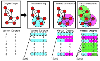
Figure 4: Application of FLFA to a graph with three communities. (top) The figures show each new community that is detected. (bottom) The list of degree ordered vertices has (multi)colored rectangles showing the (possible multiple) community membership of the vertices as new communities are detected. The seeds of each new community are indicated in the vertex lists.

The key to the FLFA is the fact that each community in a sequential community graph can be identified by finding its leaders. Since the leaders of a community only belong to one community, the neighbors of the leaders will constitute the entire community. Thus, finding the leaders associated with a community allows us to find all the members of the community.

To find leaders, FLFA makes use of the fact that the degree of a leader must be less than or equal to the degree of its neighbors, due to the fact that a leader only has connections to vertices within a single community. Thus, to find leaders, FLFA simply attempts to find vertices whose degree is less than or equal to their neighbors. Once leaders are found, their neighbors determine the underlying community structure in the graph.

FLFA uses the following approach to find leaders in a graph quickly. It orders the vertices from lowest to highest degree. Since leaders have a lower degree than followers, leaders will naturally appear earlier in the list. It then iterates through the list and finds the first vertex that has not been marked as visited yet. It marks the vertex and all of its neighbors as visited. The vertex and all of its neighbors are then placed into a community. We refer to the minimal degree vertices in a community found by the FLFA as the seeds of the community. Note that seeds are not necessarily leaders as we have define them (i.e. simplicial vertices). Rather, they represent an approximation for what the leaders may be in the observation graph. As such, the communities that are found are not necessarily cliques.

The FLFA is able to find communities in the graph extremely quickly using just a single pass through the vertices. Moreover, it is also succinct and simple in its description and implementation. Lastly, as we shall see in the results section, it still is able to find communities with a relatively high accuracy, despite taking a fraction of the time of other algorithms. We illustrate the application of the FLFA to an example graph in Figure 4. The steps of the FLFA are specified below.

procedure FLFA($G$)

     ${\mathcal{C}}\leftarrow\{\}$, $Visited\leftarrow\{\}$

     $L\leftarrow$ list of vertices of $G$ sorted by ascending degree

     for $1\leq i\leq\text{length}(L)$ do

         $v\leftarrow L[i]$

         if $v\notin Visited$ then

              $c\leftarrow v\cup\text{Neighbors}(v)$

              ${\mathcal{C}}\leftarrow{\mathcal{C}}\bigcup c$

              $Visited\leftarrow Visited\bigcup c$

         end if

     end for

     return ${\mathcal{C}}$

end procedure

IV.2 Leader-Follower Algorithm

For some graphs the FLFA is not able to find all the communities. During the construction of the sequential community graph, this occurs when new leaders enter the graph and cause leaders of a previous community to become followers. The key to discovering a leader for these hidden communities is to remove the vertices that caused the leaders of the given community to become followers. This motivates what we call the leader-follower algorithm (LFA) for community detection. This algorithm is designed to detect communities which cannot be found by the FLFA.

At each iteration of the LFA, we choose a simplicial vertex in the graph and form a community from it and its neighbors. If the community is a clique and not a subset of a previous community, we include in the set of detected communities. We then delete the vertex from the graph. This iteration is repeated until the graph is empty. With these steps, we obtain a robust algorithm that, as we will see, can exactly discover all the communities in any sequential community graph. The steps of the LFA are specified below.

procedure LFA($G$)

     ${\mathcal{C}}\leftarrow\{\}$

     while $G$ is not empty and has a simplicial vertex do

         $v=$simplicial vertex in $G$

         $c\leftarrow v\cup\text{Neighbors}(v)$

         if $c$ is a clique and $c$ is not a subset of any $c^{\prime}\in{\mathcal{C}}$ then

              ${\mathcal{C}}\leftarrow c\bigcup{\mathcal{C}}$

         end if

         $G\leftarrow G-\left\{v\right\}$

     end while

     return ${\mathcal{C}}$

end procedure

V Performance Guarantees

We will next establish theoretical performance guarantees for the LFA and FLFA. The main results presented here concern the performance of the algorithms in terms of accuracy and speed.

V.1 Accuracy

Recall that in the observation graph for a latent community graph, the communities are maximal cliques. This makes community detection for this model equivalent to finding maximal cliques. The LFA and FLFA were designed to find maximal cliques and their performance is strongest in graphs where communities take this form, such as sequential community graphs.

We first present our result for the FLFA. There are examples of sequential community graphs where the FLFA cannot find all communities. Therefore, FLFA cannot detect communities on all sequential community graphs. However, there is a subclass of sequential community graphs where the FLFA will detect all communities. Our result is as follows.

Theorem 2.

Let $G=(V,E)$ be the observation graph of a sequential community graph. The output of the FLFA applied to $G$ will contain every maximal clique of $G$ that has a leader.

Proof.

Consider an observation graph $G=(V,E)$ and let $c\subseteq V$ be a set of vertices forming a maximal clique with at least one leader. Let one of these leaders be $l$. Because $l$ is a leader, all of its neighbors are in $c$ and it has degree less than or equal to all of its neighbors. In the degree sorted list used in the FLFA, $l$ and all of its neighbors of equal degree will occur before the non-leaders in $c$. We assume without loss of generality that $l$ occurs in the degree sorted list before all other vertices in $c$. $l$ is not assigned to any community created by vertices that occur before it in the degree sorted list because it does not neighbor any of them. It is is the first vertex in $c$ that the FLFA identifies as a seed. The FLFA forms a community corresponding to $l$ and all of its neighbors, which is equivalent to $c$. Therefore, the FLFA output will contain $c$. Because this result holds for any maximal clique in $G$ with at least one leader, the FLFA output will contain all such maximal cliques. ∎

This result shows that the FLFA has exact detection on the subclass of sequential community graphs where each community has a leader, but in many sequential community graphs leaders become followers as the graph evolves. To achieve correct detection for the general class of sequential community graphs we require the LFA. Our formal result is the following.

Theorem 3.

Let $G=(V,E)$ be the observation graph of a sequential community graph. The output of LFA applied to $G$ will be the exact set of maximal cliques in $G$.

Proof.

For a sequential community graph ${\mathcal{G}}$, we define its communities as ${\mathcal{C}}$ and its observation graph as $G$. Recall that because $G$ is the observation graph of a sequential community graph, every member of ${\mathcal{C}}$ corresponds to a maximal clique in $G$. We define the output of the LFA applied to $G$ as ${\mathcal{C}}_{LFA}$. To prove Theorem 3 we show that ${\mathcal{C}}={\mathcal{C}}_{LFA}$.

Every $c\in{\mathcal{C}}$ is in ${\mathcal{C}}_{LFA}$. First we consider $c\in{\mathcal{C}}$ which has at least one leader $l$. Because $l$ is a simplicial vertex, its non-simplicial neighbors will never be deleted before it. At some iteration, $l$ (or its simplicial neighbor if exists) will be chosen to form the community with all its neighbors and be placed in ${\mathcal{C}}_{LFA}$.

Now consider $c\in{\mathcal{C}}$ which does not have a leader. To establish that this community will be found by the LFA, we first construct a clique tree for $G$. We define the clique tree $G_{C}=({\mathcal{C}},E_{C})$ with $(c_{1},c_{2})\in E_{C}$ if $c_{1}\bigcap c_{2}\neq\emptyset$. That is, each community is a vertex and there is an edge between two vertices if their corresponding communities have a non-empty intersection. In the construction of a sequential community graph we either add no new communities or add a single community which is joined by members of at most a single previous community. In the clique tree, this means that each community has at most one parent, which guarantees that it is a tree (we assume without loss of generality that $G_{C}$ is connected).

Each leaf in $G_{C}$ must have at least one leader, otherwise it would be a subset of its parent. Eventually an iteration of the LFA will find one of these leaf communities and remove one of their leaders. When all leaders are deleted, the leaf is removed from $G_{C}$, because without its leaders it is a subset of its parent and is no longer a maximal clique in the updated observation graph. Because we assumed $c$ has no leaders, it is not detected until it becomes a leaf in $G_{C}$. As the leaves are removed in the clique tree, at some iteration $c$ will become a leaf and possess a leader in the corresponding observation graph. None of the vertices in $c$ will be deleted until $c$ contains a simplicial vertex. At this iteration when $c$ is a leaf in the clique tree and has a minimal degree vertex, it is detected and placed in ${\mathcal{C}}_{LFA}$.

Every $c\in{\mathcal{C}}_{LFA}$ is in ${\mathcal{C}}$. Recall from Proposition 1 that $G$ is a recursively simplicial graph. This means that when a leader is deleted, the remaining graph will have at least one leader. Each iteration will find a community with a leader. Furthermore, this community is a maximal clique in the corresponding observation graph. Therefore, each iteration is guaranteed to find a maximal clique with at least one leader in the current observation graph.

Let $c$ be one of the communities found in an iteration of the LFA. One possibility is that $c$ is a maximal clique of the original observation graph, so $c\in{\mathcal{C}}$. The other possibility is that $c$ is a subset of a maximal clique $c^{\prime}\in{\mathcal{C}}$. In the latter case, $c$ is only a subset of $c^{\prime}$ because some vertices in $c^{\prime}$ were deleted in a previous iteration. But this can only happen if these vertices were leaders, which means $c^{\prime}$ has already been detected by the LFA, so we have $c^{\prime}\in{\mathcal{C}}_{LFA}$. ∎

V.2 Runtime

We now analyze the runtime of the FLFA and LFA. Our first result concerns the runtime of the FLFA.

Theorem 4.

For an input graph $G(V,E)$, the FLFA will terminate in $O(|E|+|V|\log(|V|))$ time.

As can be seen, the FLFA is very fast with a runtime that is linear in the graph size.

Proof.

The first step of the FLFA is to calculate the degree of each vertex and sort the vertices by degree. Calculating the degree involves counting every edge in the graph at most twice which takes $O(|E|)$ time. Sorting the $|V|$ vertices can be done in $O(|V|\log(|V|)$ time. The second step is to go through the degree sorted list and assign each unvisited vertex and its neighbors to a community. This can be done in $O(|E|)$ time. Combining these steps, we find that the a total runtime of the FLFA is $O(|E|+|V|\log(|V|))$. ∎

We have the following result for the LFA runtime.

Theorem 5.

For an input graph $G(V,E)$, the LFA will terminate in $O(|V|^{2}|E|)$ time.

The runtime of the LFA is determined by the number of iterations it requires to terminate. While the worst case bound in Theorem 5 can be potentially large, we will see in Section VI that in practice FLFA and LFA have very similar runtimes on large graphs because not many iterations of FLFA are needed.

Proof.

Each iteration of the LFA involves finding a simplicial vertex, checking if it and its neighbors form a community that is a clique and not a subset of a previous community, and then deleting this vertex from the observation graph. Finding a simplicial vertex takes $O(|E|)$ operations. Checking if a single community is a clique and a subset of a previous community will require at most $|E|$ operations, and there cannot be more than $|V|$ communities. Using this, we find that each iteration of the LFA will require $O(|V||E|)$ steps. For a graph of $|V|$ vertices, the maximum number of iterations is $|V|$. Therefore, the worst case runtime of the LFA will be $O(|V|^{2}|E|)$. ∎

VI Empirical Evaluation

We now compare the performance of the LFA and FLFA to other state of the art community detection algorithms on several real graphs. We compare the performance of the algorithms in terms of accuracy and speed on graphs with known ground truth communities. The algorithms we compare against include the method for fast modularity optimization blondel2008fast and methods based on probabilistic generative models: CESNA yangcommunity and BigClam yang2013overlapping .

VI.1 Data Description

Our dataset consist of several graphs for which we have accurate ground truth communities. We describe these graphs below. All properties of the graphs are shown in Table 1.

Graph	$|V|$	$|E|$	$|\mathcal{C}|$
Prime number graph	999	195,309	168
Culture show 2010	153	1802	13
Culture show 2011	138	3626	10
Les Miserables	71	244	80
IMDB	382,219	15,038,083	127,823

Table 1: Graph properties: Number of member vertices $|V|$, number of edges $|E|$, and number of communities $|\mathcal{C}|$.

Prime Number Graph. In a prime number graph with $N$ vertices, the integers from $2$ to $N+1>2$ are vertices, edges between two integers indicate that they share a prime number as a common factor (e.g. $14$ and $21$ have an edge since they have $7$ as a common factor), and a community corresponds to a prime number in the sense that it is a collection of integers all of which have a given prime as their factor (e.g. all integers that contain $7$ as a factor).

We use a prime number graph whose vertex set is the integers from $2$ to $1,000$. The number of ground truth communities is 168, which is the number of prime numbers less than 1,000. There is great heterogeneity in the community sizes, with some communities constituting half of the vertices, while others being isolated vertices.

Culture Show Graphs. The culture show 2010 and 2011 graphs represent performances from a college culture show at MIT in 2010 and 2011. The vertices are performers and the edges indicate whether or not two performers were in the same performance. Each performance is a separate ground truth community in this graph.

Les Miserables Graph. The Les Miserables graph captures the social interactions of the characters in the novel Les Miserables. The vertices are characters from the novel and an edge is placed between two characters if they appear in the same chapter of the novel. Each chapter corresponds to a separate ground truth community in this graph.

Internet Movie Database (IMDB) Graph.

The IMDB graph consists of actors in movies ref:imdb . Each vertex is an actor and an edge is placed between two actors if they performed in the same movie. Each ground truth community consists of actors who were all in the same movie. This graph is very large, with 382,219 vertices (actors) and 127,823 communities (movies). We will use this graph to demonstrate that our algorithms scale to larger graphs while also maintaining good accuracy.

VI.2 Experimental Results

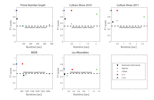
Figure 5: Plot of F1 score versus the runtime of each algorithm. The dashed line indicates the 0.5 information lower bound.

Algorithm	Prime number graph	Culture show 2010	Culture show 2011	Les Miserables	IMDB
Ground-truth	168	13	10	80	127,823
Modularity optimization	105	7	5	5	2198
BigClam	56	45	38	8	100
CESNA	2	2	2	2	2
LFA	168	13	10	34	61,059
FLFA	168	13	10	30	60,876

Table 2: Number of communities produced by each algorithm. The most accurate algorithms in terms of community number for each graph are highlighted in bold.

We compare the performance of FLFA and LFA to other algorithms on these graphs. Figure 5 shows the resulting F1 score (equation (1)) and runtimes of each algorithm.

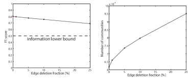
Figure 6: Plot of F1 score (top) and number of communities found (bottom) by FLFA on IMDB graph versus edge deletion fraction. The dashed line indicates the 0.5 information lower bound.

VI.2.1 Accuracy

Figure 5 shows that FLFA and LFA perform well in terms of accuracy on these graphs, consistently obtaining the highest scores. In the prime number graph, FLFA and LFA detect all communities exactly, obtaining a score of $1$, outperforming the next highest performing algorithm by $23\%$. Similarly, in the culture show graphs, FLFA and LFA again outperform the other algorithms. On both culture show graphs, FLFA and LFA both achieve a perfect score of $1$. The next best algorithm achieves a score of $0.88$ on culture show 2010 and a score of $0.79$ on culture show 2011.

In the Les Miserables graph, the LFA and FLFA have the best score of $0.65$. While this is not the perfect score we had on the prime number and culture show graphs, it is greater than the information lower bound of 0.5 given by Lemma 1. Finally, on the IMDB graph, FLFA and LFA once again detect communities extremely well. As can be seen in the table, FLFA and LFA achieve a score of $0.81$. The other algorithms are not able to even cross the information lower bound.

In addition to having the best scores, the LFA and FLFA also are the most accurate in terms of number of communities found, as seen in Table 2. In some instances, such as the IMDB graph, they are the only algorithms that come within the same order of magnitude of the number of ground-truth communities.

VI.2.2 Runtime

Not only are FLFA and LFA the most accurate algorithms on these datasets, but they are also the fastest. As shown in Figure 5, FLFA and LFA consistently perform orders of magnitude faster than alternate methods. In particular, the FLFA is able to run much faster than the other algorithms.

What is even more striking is the fact that the FLFA achieves this incredible speed with without sacrificing much in accuracy. The FLFA is the only algorithm which simultaneously has a very fast runtime and high accuracy. This is most evident on the large IMDB graph, where the FLFA has an F1 score of 0.81, which is nearly double that of the other algorithms, yet has a runtime under one second, which is almost three orders of magnitude faster than the other algorithms.

VI.2.3 Robustness

Very often we will have missing data in an observation graph. We would like to know how robust our community detection algorithms to this type of noisy observation. To check robustness, we perform the following experiment. We randomly remove different fractions of edges from the IMDB graph and apply the FLFA. The results are shown in Figure 6. As more edges are deleted, the F1 score decreases, but not substantially. With 25% of the edges removed, the score decreases by only 12.5%. This shows that the FLFA’s performance is not significantly degraded by missing data.

We saw earlier that missing data would result in spurious communities being found. From Figure 6 we see that this is indeed the case. With full observation, 61,876 communities were found by the FLFA. At 25% edge deletion, this number grows by 50%. These spurious communities generally have strong overlap with the communities found with no missing data, so even though they are numerous, their impact on the score is not as strong.

VII Conclusion

A lower bound on the F1 community score function was established in order to assess the non-triviality of the output of any community detection algorithm. This is important because many algorithms were found to produce community scores which were below this lower bound, thus bringing into question the validity of their community outputs.

We presented the leader-follower and fast leader-follower algorithms (LFA and FLFA) for fast and accurate overlapping community detection. We proposed a new generative model for community formation in social networks based on very natural social interactions. We proved that the LFA and FLFA were able to accurately learn the community structure of these models. This provided a theoretical guarantee to the performance of the algorithms.

Experiments on graphs with ground truth communities showed that the LFA and FLFA perform better than many state of the art algorithms which very often have community scores below the trivial lower bound. The FLFA was found to be almost three orders of magnitude faster than other algorithms while simultaneously maintaining high community detection accuracy. This suggests that it can be used to perform accurate, real-time community detection on extremely large graphs.

References

- [1] E. Abbe, A. S. Bandeira, and G. Hall. Exact recovery in the stochastic block model. IEEE Transactions on Information Theory, 62(1):471–487, 2016.
- [2] E. Abbe and C. Sandon. Recovering communities in the general stochastic block model without knowing the parameters. In Advances in neural information processing systems, pages 676–684, 2015.
- [3] E. M. Airoldi, D. M. Blei, S. E. Fienberg, and E. P. Xing. Mixed membership stochastic blockmodels. The Journal of Machine Learning Research, 9:1981–2014, 2008.
- [4] V. D. Blondel, J.-L. Guillaume, R. Lambiotte, and E. Lefebvre. Fast unfolding of communities in large networks. Journal of Statistical Mechanics: Theory and Experiment, 2008(10):P10008, 2008.
- [5] R. L. Breiger. The duality of persons and groups. Social forces, 53(2):181–190, 1974.
- [6] J.-J. Daudin, F. Picard, and S. Robin. A mixture model for random graphs. Statistics and computing, 18(2):173–183, 2008.
- [7] A. Decelle, F. Krzakala, C. Moore, and L. Zdeborová. Asymptotic analysis of the stochastic block model for modular networks and its algorithmic applications. Physical Review E, 84(6):066106, 2011.
- [8] S. L. Feld. The focused organization of social ties. American journal of sociology, pages 1015–1035, 1981.
- [9] C. for Complex Network Research. Network databases. http://www3.nd.edu/ networks/resources.htm, Jan. 2014.
- [10] S. Fortunato. Community detection in graphs. Physics Reports, 486(3):75–174, 2010.
- [11] B. Hajek, Y. Wu, and J. Xu. Achieving exact cluster recovery threshold via semidefinite programming. IEEE Transactions on Information Theory, 62(5):2788–2797, 2016.
- [12] M. S. Handcock, A. E. Raftery, and J. M. Tantrum. Model-based clustering for social networks. Journal of the Royal Statistical Society: Series A (Statistics in Society), 170(2):301–354, 2007.
- [13] R. Karp. Reducibility among combinatorial problems. Complexity of Computer Communications, pages 85–103, 1972.
- [14] B. Karrer and M. E. Newman. Stochastic blockmodels and community structure in networks. Physical Review E, 83(1):016107, 2011.
- [15] F. Krzakala, C. Moore, E. Mossel, J. Neeman, A. Sly, L. Zdeborová, and P. Zhang. Spectral redemption in clustering sparse networks. Proceedings of the National Academy of Sciences, 110(52):20935–20940, 2013.
- [16] E. Mossel, J. Neeman, and A. Sly. Consistency thresholds for the planted bisection model. In Proceedings of the forty-seventh annual ACM symposium on Theory of computing, pages 69–75. ACM, 2015.
- [17] M. E. Newman. Modularity and community structure in networks. Proceedings of the National Academy of Sciences, 103(23):8577–8582, 2006.
- [18] M. E. Newman and G. Reinert. Estimating the number of communities in a network. Physical review letters, 117(7):078301, 2016.
- [19] G. Palla, I. Derényi, I. Farkas, and T. Vicsek. Uncovering the overlapping community structure of complex networks in nature and society. Nature, 435(7043):814–818, 2005.
- [20] Y. Ruan, D. Fuhry, and S. Parthasarathy. Efficient community detection in large networks using content and links. In Proceedings of the 22nd international conference on World Wide Web, pages 1089–1098. ACM, 2013.
- [21] G. Simmel. Conflict and the web of group affiliations. SimonandSchuster. com, 2010.
- [22] M. J. Wainwright. Graphical models and message-passing algorithms: Some introductory lectures. In Mathematical Foundations of Complex Networked Information Systems, pages 51–108. Springer, 2015.
- [23] J. Yang and J. Leskovec. Community-affiliation graph model for overlapping network community detection. In Data Mining (ICDM), 2012 IEEE 12th International Conference on, pages 1170–1175. IEEE, 2012.
- [24] J. Yang and J. Leskovec. Overlapping community detection at scale: A nonnegative matrix factorization approach. In Proceedings of the sixth ACM international conference on Web search and data mining, pages 587–596. ACM, 2013.
- [25] J. Yang, J. McAuley, and J. Leskovec. Community detection in networks with node attributes. IEEE International Conference On Data Mining (ICDM), 2013.