The $\kern 3.00003pt\overline{\kern-1.79993ptB}{}_{d}\rightarrow\kern 1.99997pt\overline{\kern-1.99997ptK}{}^{*0}\mu^{+}\mu^{-}$ decay

Abstract

In this paper the potential for the discovery of new physics in the exclusive decay $\kern 3.00003pt\overline{\kern-1.79993ptB}{}_{d}\rightarrow\kern 1.99997pt\overline{\kern-1.99997ptK}{}^{*0}\mu^{+}\mu^{-}$ is discussed. Attention is paid to constructing observables which are protected from uncertainties in QCD form factors and at the same time observe the symmetries of the angular distribution. We discuss the sensitivity to new physics in the observables including the effect of $C\!P$-violating phases.

1 Introduction

MZ-TH/10-41

With the LHCb experiment coming online, there is the prospects of performing precision physics in the $\kern 3.00003pt\overline{\kern-1.79993ptB}{}_{d}\rightarrow\kern 1.99997pt\overline{\kern-1.99997ptK}{}^{*0}\mu^{+}\mu^{-}$ channel within a few years. This means particular attention has to be given to how the predictions from the phenomenology and the experimental measurements are compared.

First published results from BELLE [1] and BABAR [2] based on ${O}(100)$ decays already demonstrate their feasibility.

In [3], it was proposed to construct observables that maximise the sensitivity to contributions driven by the electro-magnetic dipole operator $\mathcal{O}_{7}^{{}^{\prime}}$, while, at the same time, minimising the dependence on the poorly known soft form factors.

$A_{\mathrm{T}}^{(2)}$ is highly sensitive to new right-handed currents driven by the operator $\mathcal{O}_{7}^{{}^{\prime}}$ [4], to which $A_{\mathrm{FB}}$ is blind.

Looking for the complete set of angular observables sensitive to right-handed currents, one is guided to the construction of $A_{\mathrm{T}}^{(3)}$ and $A_{\mathrm{T}}^{(4)}$ [5] and $A_{\mathrm{T}}^{(5)}$ [6]. The observables $A_{\mathrm{T}}^{(i)}$ (with $i=2,3,4,5$) use the $K^{*0}$ spin amplitudes as the fundamental building block. This provides more freedom to disentangle the information on specific Wilson coefficients than just restricting oneself to use the coefficients of the angular distribution as it was recently done in [7]. For instance, $A_{\mathrm{T}}^{(2)}$, being directly proportional to $\mathcal{C}_{7}^{{}^{\prime}}$ enhances its sensitivity to the type of NP entering this coefficient. Moreover using selected ratios of the coefficients of the distribution, like in $A_{\mathrm{T}}^{(i)}$, the sensitivity to soft form factors is completely canceled out at LO.

2 Differential decay distribution

The decay $\kern 3.00003pt\overline{\kern-1.79993ptB}{}_{d}\rightarrow\kern 1.99997pt\overline{\kern-1.99997ptK}{}^{*0}\mu^{+}\mu^{-}$, with $\kern 1.99997pt\overline{\kern-1.99997ptK}{}^{*0}\rightarrow K^{-}\pi^{+}$ on the mass shell, is completely described by four independent kinematic variables, the lepton-pair invariant mass squared, $q^{2}$, and the three angles $\theta_{l}$, $\theta_{K}$, $\phi$. Summing over the spins of the final state particles, the differential decay distribution of $\kern 3.00003pt\overline{\kern-1.79993ptB}{}_{d}\rightarrow\kern 1.99997pt\overline{\kern-1.99997ptK}{}^{*0}\ell^{+}\ell^{-}$ can be written as

$$\frac{d^{4}\Gamma}{dq^{2}\,d\cos\theta_{l}\,d\cos\theta_{K}\,d\phi}=\frac{9}{32\pi}J(q^{2},\theta_{l},\theta_{K},\phi)\,,$$ (1)

The dependence on the three angles can be made more explicit:

The $J_{i}$ depend on products of the six complex $K^{*}$ spin amplitudes, ${A_{\parallel}^{L,R}}$, ${A_{\perp}^{L,R}}$ and ${A_{0}^{L,R}}$ in the case of the SM with massless leptons. The $L$ and $R$ indicate a left and right handed current respectively. Each of these is a function of $q^{2}$. The amplitudes are just linear combinations of the well-known helicity amplitudes describing the $B\rightarrow K\pi$ transition:

$$A_{\bot,\|}^{L.R}=(H_{+1}^{L.R}\mp H_{-1}^{L.R})/\sqrt{2}\,,\qquad A_{0}^{L,R}=H_{0}^{L.R}\,.$$ (3)

The $J_{i}$ will be bi-linear functions of the spin amplitudes such as

$$J_{1s}=\frac{3}{4}\left[|{A_{\perp}^{L}}|^{2}+|{A_{\parallel}^{L}}|^{2}+|{A_{\perp}^{R}}|^{2}+|{A_{\parallel}^{R}}|^{2}\right],$$ (4)

with the expression for the eleven other $J_{i}$ terms given in [6].

The amplitudes themselves can be parametrised in terms of the seven $B\rightarrow K^{*}$ form factors by means of a narrow-width approximation. They also depend on the short-distance Wilson coefficients $\mathcal{C}_{i}$ corresponding to the various operators of the effective electroweak Hamiltonian. The precise definitions of the form factors and of the effective operators are given in [5]. Assuming only the three most important SM operators for this decay mode, namely $\mathcal{O}_{7}$, $\mathcal{O}_{9}$, and $\mathcal{O}_{10}$, and the chirally flipped ones, being numerically relevant, we have as an example

$${A_{\perp}^{L,R}}= N\sqrt{2}\lambda^{1/2}\bigg{[}\frac{V(q^{2})}{m_{B}+m_{K^{*}}}\bigg{\{}$$

$$\quad(\mathcal{C}_{9}^{\mathrm{(eff)}}+\mathcal{C}_{9}^{{}^{\prime}\mathrm{(eff)}})\mp(\mathcal{C}_{10}^{\mathrm{(eff)}}+\mathcal{C}_{10}^{{}^{\prime}\mathrm{(eff)}})\bigg{\}}+$$

$$+\frac{2m_{b}}{q^{2}}(\mathcal{C}_{7}^{\mathrm{(eff)}}+\mathcal{C}_{7}^{{}^{\prime}\mathrm{(eff)}})T_{1}(q^{2})\bigg{]}$$ (5)

where the $\mathcal{C}_{i}$ denote the corresponding Wilson coefficients, $N$ is a normalisation and

$$\lambda=m_{B}^{4}+m_{K^{*}}^{4}+q^{4}-2(m_{B}^{2}m_{K^{*}}^{2}+m_{K^{*}}^{2}q^{2}+m_{B}^{2}q^{2}).$$ (6)

There are similar expressions for the other spin amplitudes [5].

When going from the six complex spin amplitude to the expression of the angular distribution (LABEL:eq:J) with 12 $J_{i}$ terms, one would naturally assume there is no loss of information. However, it turns out that there are a number of relations between the $J_{i}$ terms; this in turns means that there are continuous transformations of the spin amplitudes that will result in the identical angular distribution. The full derivation of these symmetries can be found in [6], while here we just give the result.

In total four of the $J_{i}$ terms can be written as a function of the eight remaining $J_{i}$. Thus, the differential distribution is invariant under the following four independent symmetry transformations of the amplitudes

$$n_{i}^{{}^{\prime}}= \left[\begin{array}[]{ll}e^{i\phi_{L}}&0\\ 0&e^{-i\phi_{R}}\end{array}\right]\left[\begin{array}[]{rr}\cos\theta&-\sin\theta\\ \sin\theta&\cos\theta\end{array}\right]$$ (11)

$$\left[\begin{array}[]{rr}\cosh i\tilde{\theta}&-\sinh i\tilde{\theta}\\ -\sinh i\tilde{\theta}&\cosh i\tilde{\theta}\end{array}\right]n_{i}\,,$$ (14)

where $\phi_{L}$, $\phi_{R}$, $\theta$ and $\tilde{\theta}$ can be varied independently and $n_{i}$ is defined as

$$n_{1} =({A_{\parallel}^{L}},{A_{\parallel}^{R}}^{*})\,,$$

$$n_{2} =({A_{\perp}^{L}},-{A_{\perp}^{R}}^{*})\,,$$ (15)

$$n_{3} =({A_{0}^{L}},{A_{0}^{R}}^{*})\,.$$

Normally, there is the freedom to pick a single global phase, but as $L$ and $R$ amplitudes do not interfere here, two phases can be chosen arbitrarily as reflected in the first transformation matrix. The interpretation of the third and fourth symmetry is that they transform a helicity $+1$ final state with a left handed current into a helicity $-1$ state with a right handed current. As we experimentally cannot measure the simultaneous change of helicity and handedness of the current, these transformations turn into symmetries for the differential decay rate.

3 Comparing theory and experiment

As can be seen in the previous section it is possible to express the full angular dependence in terms of the effective Wilson coefficients. From this it would seem that it is trivially possible to extract full knowledge of the Wilson coefficients from a fit to experimental data on the angular distribution. Unfortunately there are several problems related to such an approach that will be described in turn.

As we are dealing with an exclusive decay, we have to rely on the calculation of form factors. These can come from either light cone sum rule calculations in the low $q^{2}$ region, or from lattice QCD calculations in the high $q^{2}$ region but are in both cases subject to significant uncertainty. In the low $q^{2}$ region below 6${\mathrm{\,Ge\kern-1.00006ptV^{2}\!/}c^{4}}$ the use of soft collinear effective theory (SCET), allows for the a reduction in the number of form factors from seven to two, which we will subsequently take advantage of. From below we are limited to $q^{2}>1{\mathrm{\,Ge\kern-1.00006ptV^{2}\!/}c^{4}}$ due to a logarithmic divergence in the SCET approach.

Even after the form factors have been considered, each spin amplitude has an uncertainty due to $\mathchar 28931\relax_{\mathrm{QCD}}/m_{b}$ corrections. The level of these are not known but dimensional considerations leads one to expect them at the 10% level or below. In our analysis we have made the effect explicit by illustrating the effect of $\mathchar 28931\relax_{\mathrm{QCD}}/m_{b}$ corrections at the 5% and 10% level.

The effect of charm loops will be important even outside the narrow resonance regions of the $B_{d}\rightarrow{J\mskip-3.0mu/\mskip-2.0mu\psi\mskip 2.0mu}K^{*0}$ and $B_{d}\rightarrow\psi{(2S)}K^{*0}$ due to the effect of virtual $c\overline{c}$ pairs [8]. The effect is small for $q^{2}<6{\mathrm{\,Ge\kern-1.00006ptV^{2}\!/}c^{4}}$ which is the region we consider.

When comparing theory to experimental data, two approaches are in general taken. One can start at the theory end with a physics model; from that we calculate the Wilson coefficients and subsequently the spin amplitudes. The last step will lead to a loss of accuracy due to the form factor uncertainties and the unknown $\mathchar 28931\relax_{\mathrm{QCD}}/m_{b}$ corrections. Finally we calculate the angular coefficients $J_{i}$ which can be compared directly to an angular fit of experimental data.

The other approach is to start from the experimental determination of the angular coefficients and from that determine the spin amplitudes. As we have seen in the previous section this process is not well defined due to symmetries in the angular distribution. Ignoring this point one can from the spin amplitudes get the Wilson coefficients (again suffering from form factor and $\mathchar 28931\relax_{\mathrm{QCD}}/m_{b}$ uncertainties) and go onto a physics model.

As illustrated in Fig. 1 the experimental results and the theory can be compared at several different levels. However, the uncertainties introduced in each direction means this is not optimal. We suggest instead to create a set of observables which can be derived from both the theory side and the experimental results as illustrated in Fig. 2. In this way the majority of the uncertainty due to the soft form factors can be eliminated.

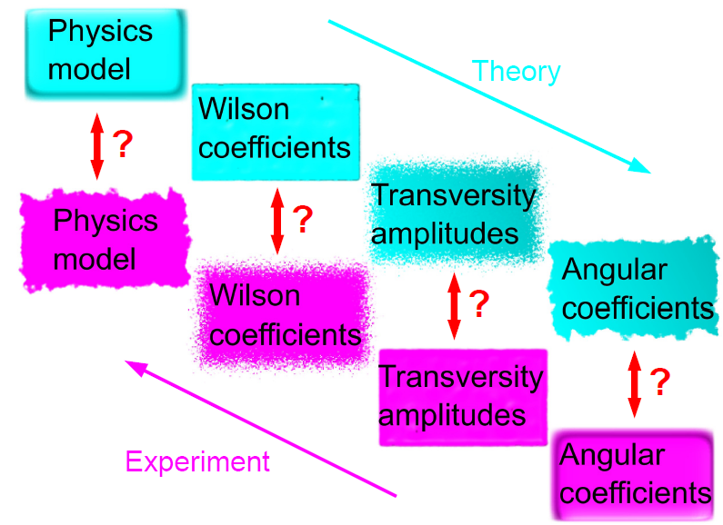
Figure 1: Traditionally experiment and theory are compared at some point along the route of transforming one to the other. For $\kern 3.00003pt\overline{\kern-1.79993ptB}{}_{d}\rightarrow\kern 1.99997pt\overline{\kern-1.99997ptK}{}^{*0}\mu^{+}\mu^{-}$ this has the disadvantage of having a large theoretical uncertainty from form factor and $\mathchar 28931\relax_{\mathrm{QCD}}/m_{b}$ uncertainties.

4 Constructing observables

When constructing observables as outlined in the previous section, several constraints has to be considered.

• They should have sensitivity to a range of new physics models. In the work we present here, we have concentrated on sensitivity to models with right handed currents, but other choices are equally possible.

• In the low $q^{2}$ region, where there are only two form factors, observables should be constructed where their value cancel out to leading order.

• The effect of $\mathchar 28931\relax_{\mathrm{QCD}}/m_{b}$ corrections should be demonstrated to be small in comparison to expected differences between the SM and different NP models.

• The observable should be invariant under the symmetries of the differential distribution described above. Otherwise it would not be well defined from an experimental point of view.

• The experimental resolution from a data set obtainable with LHCb or a super-$B$ factory should be good enough to offer distinction between models.

Based on these constraints, a range of $C\!P$-conserving observables have been designed, designated $A_{\mathrm{T}}^{(i)}$, with $i=2,3,4,5$.

An example of an observable fulfilling all the criteria is the asymmetry $A_{\mathrm{T}}^{(2)}$, first proposed in [3], and defined as

$$A_{\mathrm{T}}^{(2)}=\frac{|A_{\perp}|^{2}-|A_{\parallel}|^{2}}{|A_{\perp}|^{2}+|A_{\parallel}|^{2}},$$ (16)

where $|A_{i}|^{2}=|A_{i}^{L}|^{2}+|A_{i}^{R}|^{2}$. It has a simple form, free from form factor dependencies, in the heavy-quark ($m_{B}\rightarrow\infty$) and large $\kern 1.99997pt\overline{\kern-1.99997ptK}{}^{*0}$ energy ($E_{K^{*}}\rightarrow\infty$) limits:

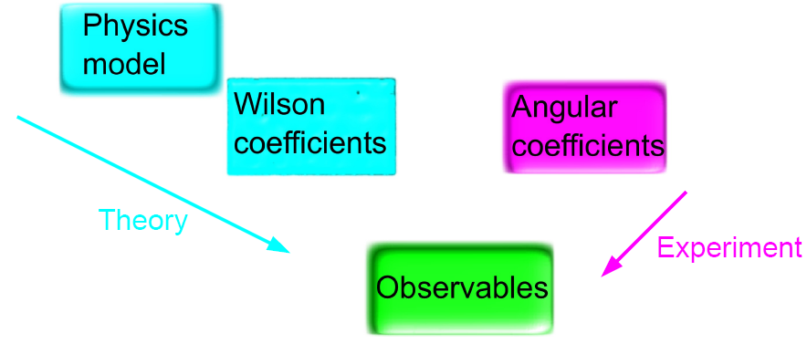
Figure 2: Observables can be constructed which from the theoretical side offers cancellation of form factors, and which from the experimental side are well defined and have good experimental sensitivity.

where $F\equiv 2m_{b}m_{B}/q^{2}$. The sensitivity to the primed Wilson coefficients corresponding to right handed currents can clearly be seen from the equation and is illustrated in Fig. 3 where a NP contribution to $\mathcal{C}_{10}^{{}^{\prime}\mathrm{(eff)}}$ is considered. It can also be seen how the theoretical errors are very small. In Fig. 4 the expected experimental resolution with data from the LHCb experiment is illustrated.

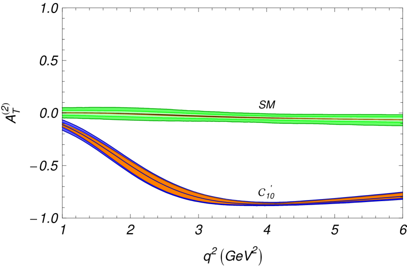
Figure 3: $A_{\mathrm{T}}^{(2)}$ in the SM (green) and with NP in $\mathcal{C}_{10}^{{}^{\prime}\mathrm{(eff)}}=3e^{i\frac{\pi}{8}}$ (blue); this value is allowed by the model independent analysis of [9]. The inner line corresponds to the central value of each curve. The dark orange bands surrounding it are the NLO results including all uncertainties (except for $\mathchar 28931\relax_{\rm QCD}/m_{b}$). Internal light green/blue bands (barely visible) include the estimated $\mathchar 28931\relax_{\rm QCD}/m_{b}$ uncertainty at a $\pm 5\%$ level and the external dark green/blue bands correspond to a $\pm 10\%$ correction for each spin amplitude.

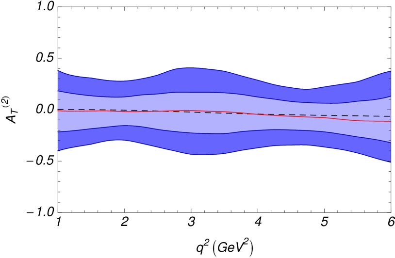
Figure 4: For $A_{\mathrm{T}}^{(2)}$ we illustrate the expected statistical experimental errors. The inner and outer bands correspond to 1$\sigma$ and 2$\sigma$ statistical errors with a yield corresponding to a 10$\mbox{\,fb}^{-1}$ data set from LHCb.

As another example,

$$A_{\mathrm{T}}^{(5)}=\frac{\big{|}{A_{\perp}^{L}}{A_{\parallel}^{R}}^{*}+{A_{\perp}^{R}}^{*}{A_{\parallel}^{L}}\big{|}}{\big{|}{A_{\perp}^{L}}\big{|}^{2}+\big{|}{A_{\perp}^{R}}\big{|}^{2}+\big{|}{A_{\parallel}^{L}}\big{|}^{2}+\big{|}{A_{\parallel}^{R}}\big{|}^{2}}\,.$$ (18)

as defined in [6], has a very different behaviour with respect to NP contributions, and a comparison of experimental measurements of $A_{\mathrm{T}}^{(2)}$ and $A_{\mathrm{T}}^{(5)}$, will be able to provide details of the underlying theory. The sensitivity to NP of $A_{\mathrm{T}}^{(5)}$ is illustrated in Fig. 5.

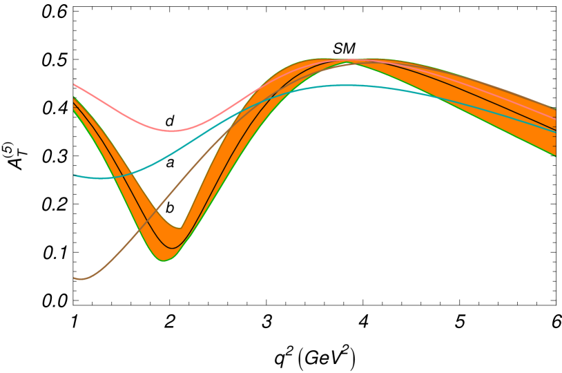
Figure 5: $A_{\mathrm{T}}^{(5)}$ in the SM and with NP in both the $\mathcal{C}_{7}^{\mathrm{(eff)}}$ and $\mathcal{C}_{7}^{{}^{\prime}\mathrm{(eff)}}$ Wilson coefficients. The cyan line ($a$) corresponds to ($\mathcal{C}_{7}^{\scriptscriptstyle{\mathrm{NP}}}$, $\mathcal{C}_{7}^{{}^{\prime}}$) = ($0.26e^{-i\frac{7\pi}{16}}$, $0.2e^{i\pi}$), the brown line ($b$) to ($0.07e^{i\frac{3\pi}{5}}$, $0.3e^{i\frac{3\pi}{5}}$) and the pink line ($d$) to ($0.18e^{-i\frac{\pi}{2}}$, $0$). The bands symbolise the theoretical uncertainty as described in Fig. 3.

5 Conclusion

We have presented how the decay $\kern 3.00003pt\overline{\kern-1.79993ptB}{}_{d}\rightarrow\kern 1.99997pt\overline{\kern-1.99997ptK}{}^{*0}\ell^{+}\ell^{-}$ can provide detailed knowledge of NP effects in the flavour sector. We developed a method for constructing observables with specific sensitivity to some types of NP while, at the same time, keeping theoretical errors from form factors under control. We demonstrate the possible impact of the unknown $\mathchar 28931\relax_{\rm QCD}/m_{b}$ corrections on the NP sensitivity of the observables. Experimental sensitivity to the observables was evaluated for datasets corresponding to 10$\mbox{\,fb}^{-1}$ of data at LHCb. A phenomenological analysis of the $A_{\mathrm{T}}^{(i)}$ observables reveals a good sensitivity to NP including the effects from $C\!P$-violating phases.

References

- [1] BELLE Collaboration, J. T. Wei et. al., Measurement of the Differential Branching Fraction and Forward-Backward Asymmetry for , Phys. Rev. Lett. 103 (2009) 171801, [arXiv:0904.0770].
- [2] BABAR Collaboration, B. Aubert et. al., Measurements of branching fractions, rate asymmetries, and angular distributions in the rare decays and , Phys. Rev. D73 (2006) 092001, [hep-ex/0604007].
- [3] F. Kruger and J. Matias, Probing new physics via the transverse amplitudes of at large recoil, Phys. Rev. D71 (2005) 094009, [hep-ph/0502060].
- [4] E. Lunghi and J. Matias, Huge right-handed current effects in in supersymmetry, JHEP 04 (2007) 058, [hep-ph/0612166].
- [5] U. Egede, T. Hurth, J. Matias, M. Ramon, and W. Reece, New observables in the decay mode , JHEP 11 (2008) 032, [arXiv:0807.2589].
- [6] U. Egede, T. Hurth, J. Matias, M. Ramon, and W. Reece, New physics reach of the decay mode , JHEP 10 (2010) 001, [1005.0571].
- [7] W. Altmannshofer et. al., Symmetries and Asymmetries of Decays in the Standard Model and Beyond, JHEP 01 (2009) 019, [arXiv:0811.1214].
- [8] A. Khodjamirian, T. Mannel, A. Pivovarov, and Y.-M. Wang, Charm-loop effect in and , 1006.4945.
- [9] C. Bobeth, G. Hiller, and G. Piranishvili, CP Asymmetries in and Untagged , Decays at NLO, JHEP 07 (2008) 106, [arXiv:0805.2525].