Irreversible Aggregation and Network Renormalization

Abstract

Irreversible aggregation is revisited in view of recent work on renormalization of complex networks. Its scaling laws and phase transitions are related to percolation transitions seen in the latter. We illustrate our points by giving the complete solution for the probability to find any given state in an aggregation process $(k+1)X\to X$, given a fixed number of unit mass particles in the initial state. Exactly the same probability distributions and scaling are found in one dimensional systems (a trivial network) and well-mixed solutions. This reveals that scaling laws found in renormalization of complex networks do not prove that they are self-similar.

Droplets beget rain, goblets coagulate to make butter or cream, and dust particles stick together to form aggregates that can eventually coalesce into planets. At the microscopic level, irreversible aggregation of atoms and molecules creates many familiar forms of matter such as aerosols, colloids, gels, suspensions, clusters and solids Zangwill (2001). Almost a century ago, Smoluchowski proposed a theory based on rate equations to describe processes governed by diffusion, collision and irreversible merging of aggregates von Smoluchowski (1917). The theory predicts how many small and large clusters exist at any given time and yields a mass distribution that depends on certain details such as the initial conditions, reactions present, relative rates, the presence or absence of spatial structure, etc. A key interest to physicists has been to derive scaling laws that characterize different universality classes (Leyvraz, 2003, and references therein).

By contrast, wide interest in complex networks Strogatz (2001); Albert and Barabási (2002); Dorogovtsev and Mendes (2002); Newman (2003) has emerged recently. Vast applications to physics, computer science, biology, and sociology (Dorogovtsev et al., 2008; Barabási, 2009; Barabási et al., 2011, and references therein) continue to be vigorously investigated. An important question is whether or not complex networks exhibit self-similarity at different length scales and if they can be grouped into universality classes on that basis. Renormalization schemes for networks were proposed Song et al. (2005); Goh et al. (2006); Kim et al. (2007); Rozenfeld et al. (2010) to address this question. Scaling of the mass or degree distribution of the renormalized nodes was used to argue that many complex networks are self-similar. The semi-sequential renormalization group (RG) flow underlying the box covering of Song et al. (2005); Goh et al. (2006); Kim et al. (2007); Rozenfeld et al. (2010) was studied carefully in Radicchi et al. (2008, 2009), where it was found that scaling laws may be related to an “RG fixed point” which was observed for a wide variety of networks. A convenient, fully sequential scheme called random sequential renormalization (RSR) was introduced Bizhani et al. (2010). At each RSR step, one node is selected at random, and all nodes within a fixed distance $\ell$ of it are replaced by a single super-node.

We point out a simple mapping between RSR and irreversible aggregation on any graph. Hence any conclusion drawn for one process holds also for the other. Indeed, a local coarse-graining step to produce a new super-node represents one aggregation event, where a ‘molecule’ aggregates with all its neighbors within distance $\ell$ to produce a new cluster. Exact analysis in one dimension reveals that even this trivial network exhibits scaling laws for the cluster mass distribution under RSR – with exponents that depend on $\ell$. Consequently, and somewhat counter-intuitively, self-similarity observed in RSR and similar network renormalization schemes cannot be used to prove that complex networks are themselves self-similar. Instead scaling laws arise due to a percolation transition in irreversible aggregation.

The correspondence between aggregation and renormalization is relevant for any model with stochastic coarse-graining of a network. For instance, the theory of space and time “Graphity” Konopka et al. (2006); Hamma et al. (2010), based on loop quantum gravity, involves a stochastic coarsening similar (albeit more structured) to RSR. Hence the critical point of aggregation may also be relevant in that and related cases. The breakdown of conventional universality, where critical exponents depend on the microscopic scale of coarse-graining, $\ell$, seems to present a dilemma for theories based on stochastic coarse-graining of a network to arrive at e.g. a universal large scale theory of gravity.

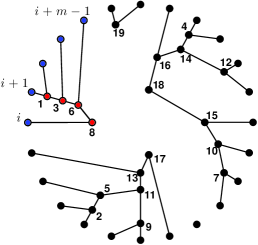
Figure 1: (Color online) Illustration of aggregation on a ring with $k=1$, $N_{0}=24$, and $N=5$. The tree in color corresponds to a cluster of mass $m=5$. It has five leaves (blue) and four internal nodes (red). Its leaves start at site $i$ and end at site $i+m-1$. The numbers beside internal nodes correspond to the time when coalescence occurs.

In order to demonstrate these points, here we consider irreversible aggregation $(k+1)X\to X$, where a randomly picked cluster coalesces with $k$ neighbors. For even $k=2\ell$ this corresponds precisely to RSR on a 1-d chain with coarsening range $\ell$. The mass of the newly formed cluster is the sum of the $(k+1)$ masses. We assume that the ‘target’ cluster is picked with uniform probability from all clusters. Other choices will be discussed in Son et al. (2011).

Let us start with the model defined on a ring, i.e., with periodic boundary conditions. Initially, $N_{0}$ sites labelled by $i\in[1,...N_{0}]$ are each occupied by a particle of mass $m=1$. Time can be either discrete or continuous, but we demand that two events never happen simultaneously. Hence events, ranked by increasing time, are denoted by positive integer values $t$. For each event, particles coagulate to form clusters of mass $m>1$. More precisely, an event consists of picking a random cluster with uniform probability and joining it with $k$ clusters to its immediate right, using periodic boundary conditions. For $k$ even, the same results are found if we aggregate clusters symmetrically. After $t$ events, $N_{t}=N_{0}-kt$ clusters exist. Our main result is the probability to find any sequence of adjacent cluster masses $p^{N_{0}}_{N_{t}}(m_{1},m_{2}\dots m_{N_{t}})$ – where a cluster of mass $m_{1}$ is followed by a cluster of mass $m_{2}$, etc., moving clockwise (see Fig. 1). we start with the single cluster mass probability.

Cluster masses are restricted to $m\equiv 1$ (mod $k$). Defining $m-1=ks$, the integer $s$ is the number of events needed to make the cluster of mass $m$. As depicted in Fig. 1, we can represent any realization of the process by a forest of $N_{t}$ rooted trees with $N_{0}$ leaves and $t$ internal nodes. Each tree $\alpha$ has $s_{\alpha}$ internal nodes, with $\sum_{\alpha}s_{\alpha}=t$. We simplify the notation by $N$ for $N_{t}$.

Let $\pi_{N}^{N_{0}}(m)$ denote, for fixed $k$ (the dependence on $k$ is not written explicitly in the following), the probability that a cluster of mass $m$ has its left-most member at site $i\in[1,N_{0}]$ after $t$ events. The probability that any of the $N$ clusters picked at random has mass $m$ is then

$$p_{N}^{N_{0}}(m)={N_{0}\over N}\;\pi_{N}^{N_{0}}(m)\quad,$$ (1)

because there are $N_{0}$ choices for $i$ and the chance to pick that particular cluster, given that it exists, is $1/N$. Since events occur completely at random, each history occurs with equal probability. The term ‘history’ refers to a fixed forest, which includes a fixed temporal order of events. Thus $\pi_{N}^{N_{0}}(m)$ is equal to the number of histories leading to a final configuration with a cluster of mass $m$ starting at position $i$, divided by all possible histories leading to $N$ clusters. The latter is equal to

$$n_{\rm hist,tot}=N_{0}\times(N_{0}-k)\times\ldots(N+k),$$ (2)

where each of the $t$ factors equals the number of choices for the next event. Using Pochhammer $k-$symbols or, equivalently, generalized rising factorials Normand (2004); Díaz and Pariguan (2007); Pitman and Picard (2006); Kingman (1982), this can be written as $n_{\rm hist,tot}=\mathbf{(}N+k\mathbf{)}_{t,k}$. Similarly, the number of histories leading to a cluster of size $m$ starting at a fixed position $i$ is

$$n_{\rm hist,cluster}=(m-k)(m-2k)\times\ldots 1=\mathbf{(}1\mathbf{)}_{s,k}$$ (3)

and the number of histories for the remaining $N-1$ clusters is

$$n_{\rm hist,rest} = (N_{0}-m-k)(N_{0}-m-2k)\times\ldots(N-1)$$ (4)

$$= \mathbf{(}N-1\mathbf{)}_{t-s,k}\quad.$$

So far we have not included the number of choices associated with different time orderings for the $s$ events in the cluster and $(t-s)$ events in the rest of the forest. The number of different time orderings is given by

$$n_{\rm orderings}={t\choose s}\quad.$$ (5)

Combining Eqs. (1) to (5), we obtain

$$p_{N}^{N_{0}}(m) = {N_{0}\over N}{t\choose s}{\mathbf{(}N-1\mathbf{)}_{t-s,k}\mathbf{(}1\mathbf{)}_{s,k}\over\mathbf{(}N+k\mathbf{)}_{t,k}}$$ (6)

$$= {t\choose s}{\mathbf{(}N-1\mathbf{)}_{t-s,k}\mathbf{(}1\mathbf{)}_{s,k}\over\mathbf{(}N\mathbf{)}_{t,k}}.$$

This result can be further simplified into beta functions or, more conveniently, $k$-beta functions (see e.g. Díaz and Pariguan (2007)),

$$B_{k}(x,y)={1\over k}B({x\over k},{y\over k})\quad,$$

giving a remarkably simple final result

$$p_{N}^{N_{0}}(m)={t\choose s}{B_{k}(N_{0}-m,m)\over B_{k}(N-1,1)}\quad.$$ (7)

We make a number of observations: (1) For $k=1$ the process maps to bond percolation on a ring. For $N=2$, the mass distribution is uniform over the entire range $m\in[1,N_{0}-1]$. For $N>2$, the distribution is proportional to the $(N-2)^{nd}$ factorial power $((N_{0}-m-1)(N_{0}-m-2)\cdots(N_{0}-m-N+2))$. (2) For $N=2$ and any $k\geq 1$, $p_{N}^{N_{0}}(m)$ is symmetric under the exchange $m\leftrightarrow N_{0}-m$. (3) For $N=2$ and $k=2$ we obtain an equation formally identical to Spitzer’s discrete arcsine law for fluctuations of random walks Spitzer (2001). (4) Asymptotic power laws for $N_{0}\to\infty$ can be determined using Stirling’s formula. If $N$ is fixed and both $m$ and $(N_{0}-m)\to\infty$,

$$p_{N}^{N_{0}}(m)\sim{(t-s)^{\frac{N-1}{k}-1}\over s^{1-\frac{1}{k}}}\quad.$$ (8)

For small masses, this gives a decreasing power law with exponent $-1+1/k$. For $N=k+1$, the power law $p_{N}^{N_{0}}(m)\sim s^{-1+1/k}$ holds up to the largest possible value, $m=N_{0}-N+1$, and the cutoff is a step function. For $m/N_{0}\to 1$ different power laws appear if $N\neq k+1$, and the sign of the exponent changes at $N=k+1$. For $N<k+1$, the distribution has a peak at $m/N_{0}\to 1$, while it goes to zero for $N>k+1$. These scaling laws are illustrated for $k=2$ in Fig. 2. (5) The scaling laws found for $m\ll N_{0}$ are identical to those obtained by Krapivsky Krapivsky (1991) for the well mixed case. However, the behavior for $m/N_{0}\to 1$ given in  Krapivsky (1991) does not agree with our result. (6) The probability $p_{N}^{N_{0}}(m)$ satisfies a number of recursion relations:

$$p_{N}^{N_{0}}(m+k)=\frac{m(N_{0}-m-N+1)}{(m+k-1)(N_{0}-m-k)}\;p^{N_{0}}_{N}(m)\;,$$

$$p^{N_{0}}_{N+k}(m)=\frac{N(N_{0}-m-N+1)}{(N-1)(N_{0}-N)}\;p^{N_{0}}_{N}(m)\;.$$

A third nonlinear recursion relation is given later.

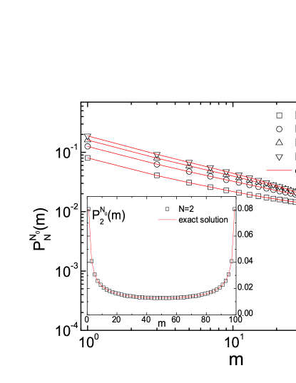
Figure 2: (Color online) Cluster size distributions after $t=50$ events for $k=2$, for different values of $N$ averaged over $10^{6}$ realizations compared to exact results. The large size behavior changes from increasing to decreasing power law at $N=k+1$. Inset: The discrete arcsine law found for $N=2$.

Joint distributions for masses of adjacent clusters can also be found. We denote by $p_{N}^{N_{0}}(m_{1},m_{2})$ the probability to find a cluster of mass $m_{1}$ followed immediately to the right by a cluster of mass $m_{2}$. This is non-zero only if $m_{1}=1+s_{1}k$ and $m_{2}=1+s_{2}k$, where $s_{\alpha}$ is the number of events needed to form a cluster of mass $m_{\alpha}$. By the same arguments that led to Eq. (6) we get

$$p_{N}^{N_{0}}(m_{1},m_{2})=\binom{t}{s_{0},s_{1},s_{2}}{\mathbf{(}N-2\mathbf{)}_{s_{0},k}\mathbf{(}1\mathbf{)}_{s_{1},k}\mathbf{(}1\mathbf{)}_{s_{2},k}\over\mathbf{(}N\mathbf{)}_{t,k}}\;,$$

where $s_{0}=t-\sum_{\beta=1}^{\alpha}s_{\beta}$ and the first factor is the multinomial coefficient instead of the binomial coefficient. When $\alpha=2$, it is a trinomial coefficient that counts the number of ways in which the three sequences of events – for the two clusters considered, and for all ($N-2$) other clusters – can be interleaved in a single history.

For any $1\leq\alpha\leq N-1$ the joint probability distribution for $\alpha$ consecutive, adjacent clusters is a product of a multinomial coefficient and $\alpha+1$ Pochhammer $k$-symbols, divided by the Pochhammer $k$-symbol related to the total number of possible histories given $N_{0}$ initial particles. Defining again $s_{0}$ as the number of events in all clusters except the first $\alpha$ ones, we can write the result compactly as

$$p_{N}^{N_{0}}(m_{1},\ldots m_{\alpha})=\binom{t}{s_{0},\ldots s_{\alpha}}{(N-\alpha)_{s_{0},k}\prod_{\beta=1}^{\alpha}(1)_{s_{\beta},k}\over(N)_{t,k}}.$$ (9)

In particular, this can also be done for the joint distribution for all $N$ masses by setting $\alpha=N-1$. The resulting expression is then manifestly invariant under any permutations of $N$ numbers $(m_{1},\ldots m_{N})$. Hence the $N-$ cluster probability is independent of the spatial ordering of the clusters. While there are obvious correlations between the mass values (the sum of all cluster masses must be $N_{0}$), there are no spatial correlations.

We now consider a line of $N_{0}$ particles with open boundaries. Again, aggregation events consist of a random choice of a cluster, followed by its amalgamation with its $k$ nearest neighbors to the right. The target cluster must be at least $k$ steps away from the right-most boundary. Following the same arguments leads immediately to Eq. (9) for $\alpha=N-1$, showing that the two models lead to precisely the same statistics.

The absence of spatial correlations indicates that the same dynamics might result for the well-mixed case. Now we start with a bucket containing $N_{0}$ balls, each of unit mass. An event consists of taking $k+1$ balls out of the bucket, merging them together, and returning the new ball to the bucket. The $k+1$ balls are chosen completely at random, independent of their masses.

The single cluster mass distribution for the well-mixed model can be obtained using the same strategy as before, but the details are quite different. Consider the total number of histories. Since events now correspond to choosing any $k+1$ balls out of $N_{0}-kt$ balls, we have, instead of the Pochhammer $k$-symbol, a product of binomial coefficients,

$$n_{\rm hist,tot}={N_{0}\choose k+1}{N_{0}-k\choose k+1}\ldots{N+k\choose k+1}.$$ (10)

The expressions for $n_{\rm hist,cluster}$ and $n_{\rm hist,rest}$ are analogous, with the factors $(m-jk)$ (resp. $(N_{0}-m-jk)$) in Eq. (3) (resp. (4)) replaced by binomial coefficients. The number of time orderings $n_{\rm orderings}$ is exactly the same as before, but the first factor $N_{0}/N$ in Eq. (6) has to be replaced by ${1\over N}{N_{0}\choose m}$. Putting all these things together, many cancellations take place, leading exactly to Eq. (7). This argument can be similarly extended to get the full $N$-particle distribution function, obtaining exactly the same result as before, for any $k$.

The time-reversed process of aggregation is fragmentation. When considering the fragmentation process associated with any of these models, we have to carefully evaluate fragmentation rates. Assuming uniform rates would not lead to all time-reversed histories having the same probability. Indeed the fraction of all mergers associated with making a cluster of mass $m^{\prime}$ is $(s^{\prime}/t)=(m^{\prime}-1)/(N_{0}-N)$, which must equal the probability that an existing cluster of mass $m^{\prime}$ will fragment at the next step in the time-reversed process. If it does, then for consistency its fragmentation products must have a mass distribution given by $p^{m^{\prime}}_{k+1}(m)$. A quadratic recursion relation for $p^{N_{0}}_{N+k}(m)$ can then be obtained by considering the likelihood of all fragmentation events in a configuration of $N$ clusters, with $m$ being the mass of one of the resulting $k+1$ fragmentation products. The relation is

$$p^{N_{0}}_{N+k}(m)=\sideset{}{{}^{\prime}}{\sum}\limits_{m^{\prime}=m+k}^{N_{0}-N+1}{N(m^{\prime}-1)p^{N_{0}}_{N}(m^{\prime})p^{m^{\prime}}_{k+1}(m)\over N_{0}-N},$$

where the prime on the summation symbol indicates that $m^{\prime}$ must increase in steps of $k$.

In summary, we derived complete solutions for the probability to find any given state in three models – well-mixed solutions, particles on a ring reacting with their $k$ nearest neighbors, and the same reaction for particles on a line with open boundaries – and show that these solutions are precisely the same. The fact that we could solve exactly a one dimensional model without detailed balance might seem surprising since such models are in general not solvable. It stems from the fact that spatial correlations, although a priori not excluded, are in fact absent. Related to this is our finding that the well-mixed models have exactly the same solutions. Our method can be used to solve the model where the target cluster is picked with a probability proportional to its mass Son et al. (2011). Perhaps generalizations of these observations hold true for more complicated models, in which case weighted path integrals would replace sums over histories.

We have pointed out a direct mapping between irreversible aggregation and RSR. The latter was motivated by claims that one can define finite fractal dimensions for real networks Song et al. (2005), using similar but more complicated and ambiguous schemes. Results for RSR with $\ell=1$ on various graphs (critical trees Bizhani et al. (2010), Erdös-Renyi and Barabasi-Albert networks Bizhani et al. (2011), and regular lattices Christensen et al. (2010)) concur with our present conclusions for $k=2$. Apart from studying a system that is sufficiently simple to be exactly solvable and that is obviously not fractal, here we presented results for $\ell>1$, showing that scaling laws depend in a non-trivial way on $\ell$. Results for the elementary network (a one dimensional line) examined analytically here proves that scaling under stochastic network renormalization arises from an underlying percolation transition in aggregation and does not prove fractality or self-similarity of the underlying graph.

Our mapping suggests that the critical behavior of aggregation may also turn up in “Graphity” Konopka et al. (2006); Hamma et al. (2010) or related models, where geometry, gravity, and matter emerge through an aggregation process of an underlying graph. “Geometrogenesis” is the complementary process of infinite cluster formation in irreversible aggregation. In that case, scaling that depends on the microscopic coarse-graining scale $\ell$ seems to add further obstacles to the persistent and challenging problem to derive a large scale theory of gravity from microscopic graph models.

References

- Zangwill (2001) A. Zangwill, Nature 411, 651 (2001).
- von Smoluchowski (1917) M. von Smoluchowski, Z. Phys. Chem. 92, 129 (1917).
- Leyvraz (2003) F. Leyvraz, Phys. Rep. 383, 95 (2003).
- Strogatz (2001) S. H. Strogatz, Nature 410, 268 (2001).
- Albert and Barabási (2002) R. Albert and A.-L. Barabási, Rev. Mod. Phys. 74, 47 (2002).
- Dorogovtsev and Mendes (2002) S. N. Dorogovtsev and J. F. F. Mendes, Adv. Phys. 51, 1079 (2002).
- Newman (2003) M. E. J. Newman, SIAM Rev. 45, 167 (2003).
- Dorogovtsev et al. (2008) S. N. Dorogovtsev, A. V. Goltsev, and J. F. F. Mendes, Rev. Mod. Phys. 80, 1275 (2008).
- Barabási (2009) A.-L. Barabási, Science 24, 412 (2009).
- Barabási et al. (2011) A.-L. Barabási, N. Gulbahce, and J. Loscalzo, Nature Rev. Genet. 12, 56 (2011).
- Song et al. (2005) C. Song, S. Havlin, and H. Makse, Nature 433, 392 (2005).
- Goh et al. (2006) K.-I. Goh, G. Salvi, B. Kahng, and D. Kim, Phys. Rev. Lett. 96, 018701 (2006).
- Kim et al. (2007) J. S. Kim et al., Phys. Rev. E 75, 16110 (2007).
- Rozenfeld et al. (2010) H. Rozenfeld, C. Song, and H. Makse, Phys. Rev. Lett. 104, 25701 (2010).
- Radicchi et al. (2008) F. Radicchi, J. J. Ramasco, A. Barrat, and S. Fortunato, Phys. Rev. Lett. 101, 148701 (2008).
- Radicchi et al. (2009) F. Radicchi, A. Barrat, S. Fortunato, and J. J. Ramasco, Phys. Rev. E 79, 26104 (2009).
- Bizhani et al. (2010) G. Bizhani, V. Sood, M. Paczuski, and P. Grassberger, e-print arXiv:1009.3955, to appear in Phys. Rev. E (2010).
- Konopka et al. (2006) T. Konopka, F. Markopoulou, and L. Smolin, e-print arXiv:hep-th/0611197v1 (2006).
- Hamma et al. (2010) A. Hamma et al., Phys. Rev. D 81, 104032 (2010).
- Son et al. (2011) S.-W. Son et al., in preparation (2011).
- Normand (2004) J. Normand, J. Phys. A 37, 5737 (2004).
- Díaz and Pariguan (2007) R. Díaz and E. Pariguan, Divulg. Mat. 15, 179 (2007).
- Pitman and Picard (2006) J. Pitman and J. Picard, Combinatorial stochastic processes (Springer, 2006).
- Kingman (1982) J. Kingman, J. Appl. Prob. 19, 27 (1982).
- Spitzer (2001) F. Spitzer, Principles of random walk (Springer Verlag, 2001).
- Krapivsky (1991) P. Krapivsky, J. Phys. A 24, 4697 (1991).
- Bizhani et al. (2011) G. Bizhani et al., in preparation (2011).
- Christensen et al. (2010) C. Christensen et al., e-print arXiv:1012.1070 (2010).