A posteriori error estimator based on gradient recovery by averaging for convection-diffusion-reaction problems approximated by discontinuous Galerkin methods

Abstract

We consider some (anisotropic and piecewise constant) convection-diffusion-reaction problems in domains of $\mbox{\Blackbrd R}^{2}$, approximated by a discontinuous Galerkin method with polynomials of any degree. We propose two a posteriori error estimators based on gradient recovery by averaging. It is shown that these estimators give rise to an upper bound where the constant is explicitly known up to some additional terms that guarantees reliability. The lower bound is also established, one being robust when the convection term (or the reaction term) becomes dominant. Moreover, the estimator is asymptotically exact when the recovered gradient is superconvergent. The reliability and efficiency of the proposed estimators are confirmed by some numerical tests.

Key Words convection-diffusion-reaction problems, a posteriori estimator, discontinuous Galerkin finite elements.

AMS (MOS) subject classification 65N30; 65N15, 65N50.

1 Introduction

The finite element method is the more popular one that is commonly used in the numerical realization of different problems appearing in engineering applications, like the Laplace equation, the Lamé system, the Stokes system, the Maxwell system, etc…. (see [7, 8, 26]). More recently discontinuous Galerkin finite element methods become very attractive since they present some advantages. For example, they allow to perform ”$p$ refinement”, by locally increasing the polynomial degree of the approximation if needed. They can moreover use non-conform meshes allowing hanging-nodes, making the mesh generation easier for concrete industrial applications. We refer to [3, 10], and the references cited there, for a good overview on this topic. Adaptive techniques based on a posteriori error estimators have become indispensable tools for such methods. For continuous Galerkin finite element methods, there now exists a vast amount of literature on a posteriori error estimation for problems in mechanics or electromagnetism and obtaining locally defined a posteriori error estimates, see for instance the monographs [2, 4, 27, 35]. On the other hand a similar theory for discontinuous methods is less developed, let us quote [5, 12, 13, 20, 21, 22, 30, 34].

Usually upper and lower bounds are proved in order to guarantee the reliability and the efficiency of the proposed estimator. Most of the existing approaches involve constants depending on the shape regularity of the elements and/or of the jumps in the coefficients; but these dependences are often not given. Only a small number of approaches gives rise to estimates with explicit constants, let us quote [2, 6, 18, 23, 25, 28, 29] for continuous methods. For discontinuous methods, we may cite the recent papers [1, 9, 13, 15, 16, 24].

Our goal is here to consider convection-diffusion-reaction problems with discontinuous diffusion coefficients in two-dimensional domains with Dirichlet boundary conditions approximated by a discontinuous Galerkin method with polynomials of any degree. Inspired from the paper [18], which treats the case of continuous diffusion coefficients approximated by a continuous Galerkin method, we further derive some a posteriori estimators with an explicit constant in the upper bound (1 or a similar constant) up to some additional terms that are usually superconvergent and some oscillating terms. The approach, called gradient recovery by averaging [18] is based on the construction of a Zienkiewicz/Zhu estimator, namely the difference in an appropriate norm of $a\nabla_{h}u_{h}-Gu_{h}$, where $\nabla_{h}u_{h}$ is the broken gradient of $u_{h}$ and $Gu_{h}$ is a $H({\rm{div}\,})$-conforming approximation of this variable. Here special attention has to be paid due to the assumption that $a$ may be discontinuous. Moreover the non conforming part of the error is managed using a comparison principle from [16] and a standard Oswald interpolation operator [1, 22]. Furthermore using standard inverse inequalities, we show that our estimator is locally efficient. Two interests of this approach are first the simplicity of the construction of $Gu_{h}$, and secondly its superconvergence property (validated by numerical tests). Let us finally notice that this paper extends our previous one [13] in many directions: first we treat convection-diffusion-reaction problems instead of purely diffusion ones. Second we track the dependence of the constant in the lower bounds, in particular we show that the natural extension of the estimator from [13] yields a lower bound with a constant that is not robust when the convection and/or the reaction term becomes dominant. Consequently we introduce another estimator (adapted from [36]) that is robust, keeping nevertheless an upper bound with an explicit constant.

The schedule of the paper is as follows: We recall in section 2 the convection-diffusion-reaction problem, its numerical approximation and recall the comparison principle from [16]. Section 3 is devoted to the introduction of the first estimator based on gradient averaging and the proofs of the upper and lower bounds. The upper bound directly follows from the construction of the estimator and some results from [18], while the lower bound requires the use of some inverse inequalities and a special construction of $Gu_{h}$. Since the lower bound is not robust as the convection and/or the reaction term becomes dominant we propose an alternative estimator in section 4 and show its robustness. Finally in section 5 some numerical tests are presented that confirm the reliability and efficiency of our estimators and the superconvergence of $Gu_{h}$ to $a\nabla u$.

Let us finish this introduction with some notation used in the remainder of the paper: On $D$, the $L^{2}(D)$-norm will be denoted by $\|\cdot\|_{D}$. In the case $D=\Omega$, we will drop the index $\Omega$. The usual norm and semi-norm of $H^{s}(D)$ ($s\geq 0$) are denoted by $\|\cdot\|_{s,D}$ and $|\cdot|_{s,D}$, respectively. Finally, the notation $a\lesssim b$ and $a\sim b$ means the existence of positive constants $C_{1}$ and $C_{2}$, which are independent of the mesh size, the coefficients of the operator and of the quantities $a$ and $b$ under consideration such that $a\lesssim C_{2}b$ and $C_{1}b\lesssim a\lesssim C_{2}b$, respectively. In other words, the constants may depend on the aspect ratio of the mesh, as well as the polynomial degree $l$, but they do not depend on the coefficients of the operator $a,\beta$ and $\mu$ (see below).

2 The boundary value problem and its discretization

Let $\Omega$ be a bounded domain of $\mbox{\Blackbrd R}^{2}$ with a Lipschitz boundary $\Gamma$ that we suppose to be polygonal. We consider the following convection-diffusion-reaction problem with homogeneous Dirichlet boundary conditions:

$$\left\{\begin{array}[]{rcl}-{\rm{div}\,}(a\hbox{~{}}\nabla u)+\beta\cdot\nabla u+\mu u&=&f\mbox{~{}in~{}$\Omega$},\\ u&=&0\hbox{~{}on~{}$\Gamma$}.\end{array}\right.$$ (1)

In the sequel, we suppose that $a$ is a symmetric positive definite matrix which is piecewise constant, namely we assume that there exists a partition $\cal P$ of $\Omega$ into a finite set of Lipschitz polygonal domains $\Omega_{1},\cdots,\Omega_{J}$ such that, on each $\Omega_{j}$, $a=a_{j}$ where $a_{j}$ is a symmetric positive definite matrix. Furthermore we assume that $\beta\in H({\rm{div}\,},\Omega)\cap L^{\infty}(\Omega)^{2}$, $\mu\in L^{\infty}(\Omega)$ and are such that $\mu-\frac{1}{2}{\rm{div}\,}\beta\geq 0$. If $\mu-\frac{1}{2}{\rm{div}\,}\beta=0$ on $\omega\subset\Omega$, then we assume that $\mu={\rm{div}\,}\beta=0$ on $\omega$.

The variational formulation of (1) involves the bilinear form

$${\it B}(u,v)=\int_{\Omega}(a\nabla u\cdot\nabla v+\beta\cdot\nabla uv+\mu uv),\forall u,v\in H^{1}_{0}(\Omega),$$

and the corresponding energy norm

$$|||v|||^{2}={\it B}(v,v)=\int_{\Omega}(a\nabla v\cdot\nabla v+(\mu-\frac{1}{2}{\rm{div}\,}\beta)|v|^{2}),\forall v\in H^{1}_{0}(\Omega).$$

Given $f\in L^{2}(\Omega)$, the weak formulation consists in finding $u\in H^{1}_{0}(\Omega)$ such that

$${\it B}(u,v)=(f,v),\hbox{~{}}\forall v\in H^{1}_{0}(\Omega),$$ (2)

where $(f,v)$ means the $L^{2}$ inner product in $\Omega$, i.e., $(f,v)=\int_{\Omega}fv$. Invoking the positiveness of $a$ and the hypothesis $(\mu-\frac{1}{2}{\rm{div}\,}\beta)\geq 0$, the bilinear form ${\it B}$ is coercive on $H^{1}_{0}(\Omega)$ with respect to the norm $|||\cdot|||$ and this coerciveness guarantees that problem (2) has a unique solution by the Lax-Milgram lemma.

2.1 Discontinuous Galerkin approximated problem

Following [3, 16, 22], we consider the following discontinuous Galerkin approximation of our continuous problem: We consider a triangulation ${\mathcal{T}}$ made of triangles $T$ whose edges are denoted by $e$. We assume that this triangulation is regular, i.e., for any element $T$, the ratio $\displaystyle\frac{h_{T}}{\rho_{T}}$ is bounded by a constant $\sigma>0$ independent of $T$ and of the mesh size $h=\max_{T\in{\mathcal{T}}}h_{T}$, where $h_{T}$ is the diameter of $T$ and $\rho_{T}$ the diameter of its largest inscribed ball. We further assume that ${\mathcal{T}}$ is conforming with the partition $\cal P$ of $\Omega$, i.e., the matrix $a$ being constant on each $T\in{\mathcal{T}}$, we then denote by $a_{T}$ the value of $a$ restricted to an element $T$. With each edge $e$ of an element $T$, we associate its length $h_{e}$ and a unit normal vector $n_{e}$, while $n_{T}$ stands for the outer unit normal vector along $\partial T$. ${\mathcal{E}}$ (resp. ${\mathcal{N}}$) represents the set of edges (resp. vertices) of the triangulation. In the sequel, we need to distinguish between edges (resp. vertices) included into $\Omega$ or into $\Gamma$, in other words, we set

$${\mathcal{E}}_{int} = \{e\in{\mathcal{E}}:e\subset\Omega\},{\mathcal{N}}_{int}=\{x\in{\mathcal{N}}:x\in\Omega\},$$

$${\mathcal{E}}_{D} = \{e\in{\mathcal{E}}:e\subset\Gamma\},{\mathcal{N}}_{D}=\{x\in{\mathcal{N}}:x\in\Gamma\}.$$

Problem (2) is approximated by the (discontinuous) finite element space:

$$X_{h}=\left\{v_{h}\in L^{2}(\Omega)|{v_{h}}_{|T}\in\mbox{\Blackbrd P}_{\ell}(T),T\in{\mathcal{T}}\right\},$$

where $\ell$ is a fixed positive integer. Later on we also need the continuous counterpart of $X_{h}$, namely we introduce

$$S_{h}=\left\{v_{h}\in C(\overline{\Omega})|{v_{h}}_{|T}\in\mbox{\Blackbrd P}_{\ell}(T),T\in{\mathcal{T}}\right\},$$

as well as

$$S_{h,1}=\left\{v_{h}\in C(\overline{\Omega})|{v_{h}}_{|T}\in\mbox{\Blackbrd P}_{1}(T),T\in{\mathcal{T}}\right\}.$$

We further need

$$X_{h,1}=\left\{v_{h}\in L^{2}(\Omega)|{v_{h}}_{|T}\in\mbox{\Blackbrd P}_{1}(T),T\in{\mathcal{T}}\right\}.$$

For our further analysis we need to define some jumps and means through any edge $e\in{\mathcal{E}}$ of the triangulation. For $e\in{\mathcal{E}}_{int}$, we denote by $T^{+}$ and $T^{-}$ the two elements of ${\mathcal{T}}$ containing $e$. Let $q\in X_{h}$, we denote by $q^{\pm}$, the traces of $q$ taken from $T^{\pm}$, respectively. Then we define the mean of $q$ on $e$ by

$$\mbox{$\big{\{}\big{\{}q\big{\}}\big{\}}$}_{\omega}=\omega^{+}(e)q^{+}+\omega^{-}(e)q^{-},$$

where the nonnegative weights $\omega^{\pm}(e)$ have to satisfy $\omega^{+}(e)+\omega^{-}(e)=1$. If $\omega^{+}(e)=\omega^{-}(e)=1/2$, we drop the index $\omega$. The jump of $q$ on $e$ is now defined as follows:

$$\mbox{$\big{[}\big{[}q\big{]}\big{]}$}=q^{+}n_{T^{+}}+q^{-}n_{T^{-}}.$$

Remark that the jump $\big{[}\big{[}q\big{]}\big{]}$ of $q$ is vector-valued.

For $v\in[X_{h}]^{d}$, we denote similarly

$$\mbox{$\big{\{}\big{\{}v\big{\}}\big{\}}$}_{\omega}=\omega^{+}(e)v^{+}+\omega^{-}(e)v^{-}.$$

For a boundary edge $e$, i. e. $e\in{\mathcal{E}}_{D}$, there exists a unique element $T^{+}\in{\mathcal{T}}$ such that $e\subset\partial T^{+}$. Therefore the mean and jump of $q$ are defined by $\mbox{$\big{\{}\big{\{}q\big{\}}\big{\}}$}=q^{+}$ and $\mbox{$\big{[}\big{[}q\big{]}\big{]}$}=q^{+}n_{T^{+}}$.

For $q\in X_{h}$, we define its broken gradient $\nabla_{h}q$ in $\Omega$ by :

$$(\nabla_{h}q)_{|T}=\nabla q_{|T},\forall T\in{\mathcal{T}}.$$

For $w\in X_{h}+H^{1}_{0}(\Omega)$ and for $\omega\subset\Omega$, we set

$$|||w|||_{T}^{2} = \int_{T}(a\nabla w\cdot\nabla w+(\mu-\frac{1}{2}{\rm{div}\,}\beta)|w|^{2}),\forall T\in{\mathcal{T}},$$

$$|||w|||^{2}_{\omega} = \sum_{T\in{\mathcal{T}}:T\subset\bar{\omega}}|||w|||_{T}^{2},\quad|||w|||^{2}=\sum_{T\in{\mathcal{T}}}|||w|||_{T}^{2},$$

$$\|w\|_{DG,h} = |||w|||+\left(\sum_{e\in{\mathcal{E}}}h_{e}^{-1}\|\mbox{$\big{[}\big{[}w\big{]}\big{]}$}\|^{2}_{e}\right)^{1/2}.$$

Note that $\|\cdot\|_{DG,h}$ is a norm on $X_{h}$.

With these notations, we define the bilinear form ${\it B}_{h}(.,.)$ as follows:

$${\it B}_{h}(u_{h},v_{h}) = (a\nabla_{h}u_{h},\nabla_{h}v_{h})+((\mu-{\rm{div}\,}\beta)u_{h},v_{h})-(u_{h},\beta\cdot\nabla_{h}v_{h})$$

$$- \sum_{e\in{\mathcal{E}}}\int_{e}(\theta\mbox{$\big{\{}\big{\{}a\nabla_{h}v_{h}\big{\}}\big{\}}$}_{\omega}\cdot\mbox{$\big{[}\big{[}u_{h}\big{]}\big{]}$}+\mbox{$\big{\{}\big{\{}a\nabla_{h}u_{h}\big{\}}\big{\}}$}_{\omega}\cdot\mbox{$\big{[}\big{[}v_{h}\big{]}\big{]}$})$$

$$+ \sum_{e\in{\mathcal{E}}}\int_{e}(\gamma_{e}\mbox{$\big{[}\big{[}u_{h}\big{]}\big{]}$}\cdot\mbox{$\big{[}\big{[}v_{h}\big{]}\big{]}$}+\mbox{$\big{\{}\big{\{}u_{h}\big{\}}\big{\}}$}\beta\cdot\mbox{$\big{[}\big{[}v_{h}\big{]}\big{]}$}),\qquad\forall u_{h},v_{h}\in X_{h},$$

where $\theta$ is a fixed real parameter and the positive parameters $\gamma_{e}$ are chosen appropriately, see below.

The discontinuous Galerkin approximation of problem (2) reads now: Find $u_{h}\in X_{h}$, such that

$${\it B}_{h}(u_{h},v_{h})=(f,v_{h}),\mbox{~{}}\forall v_{h}\in X_{h}.$$ (4)

In (2.1), taking the interior weights $\omega^{\pm}(e)$ equal to $1/2$ and setting $\theta=0$, $\theta=-1$ or $\theta=1$ leads to the incomplete, nonsymmetric or symmetric interior-penalty discontinuous Galerkin methods. The stabilization parameters $\gamma_{e}$ are chosen in the form (see e.g. [16, 17])

$$\gamma_{e}=\alpha_{e}\frac{\gamma_{a,e}}{h_{e}}+\gamma_{\beta,e},$$ (5)

where $\alpha_{e}$ is a positive parameter, $\gamma_{a,e}$ is a positive parameter that depends on $a$ and $\gamma_{\beta,e}$ is a positive parameter that depends on $\beta$ and is zero is $\beta=0$ (the choice $\gamma_{\beta,e}=\frac{|\beta\cdot n_{e}|}{2}$ corresponding to an upwinding scheme). Whenever $\theta\neq-1$, the parameters $\alpha_{e}$ have to be large enough to ensure coerciveness of the bilinear form ${\it B}_{h}$ on $X_{h}$ (see, e.g., Lemma 2.1 of [22]).

If $\omega$ is a subset of $\Omega$, we denote by $c_{a,\omega}$ (resp. $C_{a,\omega}$) the minimal (resp. maximal) eigenvalue of the restriction of the matrix $a$ to $\omega$. We further denote by $c_{\beta,\mu,\omega}=\inf_{x\in\omega}(\mu-\frac{1}{2}{\rm{div}\,}\beta)$. We recall that from our assumption, we have the implication

$$c_{\beta,\mu,\omega}=0\Rightarrow{\rm{div}\,}\beta=0\hbox{ and }\mu=0\hbox{ in }\omega.$$

For shortness we drop the index $\Omega$ in these notations, namely we set $c_{a}=c_{a,\Omega}$, $C_{a}=C_{a,\Omega}$ and $c_{\beta,\mu}=c_{\beta,\mu,\Omega}$.

As our approximated scheme is a non conforming one (i.e. the solution does not belong to $H^{1}_{0}(\Omega)$), as usual we need to take into account the non conforming part of the error. The possibilities are twofold : either use an appropriate Helmholtz decomposition of the error (see Lemma 3.2 of [14], or Theorem 1 of [1] in 2D or Lemma 2.1 of [9]) or use the following comparison principle, proved in Theorem 6.3 of [16].

Lemma 2.1 (Abstract upper error bound)

Let $u\in H^{1}_{0}(\Omega)$ be a solution of (2) and $u_{h}\in X_{h}$ be the solution of (4), then

$$|||u-u_{h}|||\leq\inf_{s\in H^{1}_{0}(\Omega)}\Big{\{}|||u_{h}-s|||$$

$$+ \inf_{{\mathbf{t}}\in H({\rm{div}\,},\Omega)}\sup_{\varphi\in H^{1}_{0}(\Omega):|||\varphi|||=1}\Big{(}(f-{\rm{div}\,}{\mathbf{t}}-\beta\cdot\nabla s-\mu s,\varphi)$$

$$- (a\nabla_{h}u_{h}+{\mathbf{t}},\nabla\varphi)+((\mu-\frac{1}{2}{\rm{div}\,}\beta)(s-u_{h}),\varphi)\Big{)}\Big{\}}.$$

3 The a posteriori error analysis based on gradient recovery by averaging

Error estimators can be constructed in many different ways as, for example, using residual type error estimators which measure locally the jump of the discrete flux [22]. A different method, based on equilibrated fluxes, consists in solving local Neumann boundary value problems [2] or in using Raviart-Thomas interpolant [1, 9, 15, 16]. Here, as an alternative we introduce a gradient recovery by averaging and define an error estimator based on a $H({\rm{div}\,})$-conforming approximation of the broken gradient $a\nabla_{h}u_{h}$. In comparison with [18], we admit discontinuous diffusion coefficients and use a discontinuous Galerkin method.

Inspired from [18] the conforming part of the estimator $\eta_{CF}$ involves the difference between the broken gradient $a\nabla_{h}u_{h}$ and its smoothed version $Gu_{h}$, where $Gu_{h}$ is for the moment any element in $X_{h,1}^{2}$ satisfying

$$Gu_{h}\in H({\rm{div}\,},\Omega)=\{v\in L^{2}(\Omega)^{2}:{\rm{div}\,}v\in L^{2}(\Omega)\},$$ (7)

$$(Gu_{h})|_{|\Omega_{j}}\in H^{1}(\Omega_{j}),\forall j=1,\cdots,J.$$ (8)

Hence conforming part of the estimator $\eta_{CF}$ is defined by

$$\eta_{CF}^{2}=\sum_{T\in{\mathcal{T}}}\eta_{CF,T}^{2},$$ (9)

where the indicator $\eta_{CF,T}$ is defined by

$$\eta_{CF,T}=\|a^{-1/2}\left(a\nabla u_{h}-Gu_{h}\right)\|_{T}.$$

For the nonconforming part of the error, we associate with $u_{h}$, its Oswald interpolation operator, namely the unique element $I_{\rm Os}u_{h}\in S_{h}$ defined in the following natural way (see Theorem 2.2 of [22]): to each node $n$ of the mesh corresponding to the Lagrangian-type degrees of freedom of $S_{h}$, the value of $I_{\rm Os}u_{h}$ is the average of the values of $u_{h}$ at this node $n$ if it belongs to $\Omega$ (i.e., $I_{\rm Os}u_{h}(n)=\frac{\sum_{n\in T}|T|u_{h|T}(n)}{\sum_{n\in T}|T|}$) and is zero at this node if it belongs to $\Gamma$. Then the non conforming indicator $\eta_{NC,T}$ is simply

$$\eta_{NC,T}=|||I_{\rm Os}u_{h}-u_{h}|||_{T}=(||a^{1/2}\nabla(I_{\rm Os}u_{h}-u_{h})\|_{T}^{2}+||(\mu-\frac{1}{2}{\rm{div}\,}\beta)^{1/2}(I_{\rm Os}u_{h}-u_{h})\|_{T}^{2})^{\frac{1}{2}}.$$

The non conforming part of the estimator is then

$$\eta_{NC}^{2}=\sum_{T\in{\mathcal{T}}}\eta_{NC,T}^{2}.$$ (10)

Similarly by keeping in $\eta_{NC}$ only the zero order term, we get a second non conforming indicator $\eta_{NC2,T}$, which is simply

$$\eta_{NC2,T}=||(\mu-\frac{1}{2}{\rm{div}\,}\beta)^{1/2}(I_{\rm Os}u_{h}-u_{h})\|_{T},$$

with a global contribution

$$\eta_{NC2}^{2}=\sum_{T\in{\mathcal{T}}}\eta_{NC2,T}^{2}.$$ (11)

We obviously notice that

$$\eta_{NC2,T}\leq\eta_{NC,T}.$$

Similarly we introduce the estimator corresponding to jumps of $u_{h}$:

$$\eta_{J}^{2}=\sum_{e\in{\mathcal{E}}}\eta_{J,e}^{2},$$

with

$$\eta_{J,e}^{2}=\left\{\begin{tabular}[]{ll}$h_{e}^{-1}\|\mbox{$\big{[}\big{[}u_{h}\big{]}\big{]}$}\|_{e}^{2}$&if $e\in{\mathcal{E}}_{int}$,\vspace{2mm}\\ $h_{e}^{-1}\|u_{h}\|_{e}^{2}$&if $e\in{\mathcal{E}}_{D}$.\end{tabular}\right.$$

As in [18], we introduce some additional superconvergent security parts. In order to define them properly we recall that for a node $x\in{\mathcal{N}}$, we denote by $\lambda_{x}$ the standard hat function (defined as the unique element in $S_{h,1}$ such that $\lambda_{x}(y)=\delta_{x,y}$ for all $y\in{\mathcal{N}}$), let $\omega_{x}$ be the patch associated with $x$, which is simply the support of $\lambda_{x}$ and let $h_{x}$ be the diameter of $\omega_{x}$ (which is equivalent to the diameter $h_{K}$ of any triangle $K$ included into $\omega_{x}$). We now denote by $r$ the element residual

$$r=f+{\rm{div}\,}(Gu_{h})-\beta\cdot\nabla I_{\rm Os}u_{h}-\mu I_{\rm Os}u_{h}$$

and for all $x\in{\mathcal{N}}$, we set

$$\bar{r}_{x}= \big{(}\int_{\omega_{x}}\lambda_{x}\big{)}^{-1}\int_{\omega_{x}}r\lambda_{x} \hbox{ if }x\in{\mathcal{N}}_{int}={\mathcal{N}}\setminus{\mathcal{N}}_{D},$$

$$\bar{r}_{x}= 0 \hbox{ if }x\in{\mathcal{N}}_{D}.$$

We further use a multilevel decomposition of $S_{h,1}$, namely we suppose that we start from a coarse grid ${\mathcal{T}}_{0}$ and that the successive triangulations are obtained by using the bisection method, see [18, 32]. This means that we obtain a finite sequence of nested triangulations ${\mathcal{T}}_{\ell}$, $\ell=0,\cdots,L$ such that ${\mathcal{T}}_{L}={\mathcal{T}}$. Denoting by $S_{\ell}$ the space

$$S_{\ell}=\left\{v\in C(\overline{\Omega})|{v}_{|T}\in\mbox{\Blackbrd P}_{1}(T),T\in{\mathcal{T}}_{\ell}\right\},$$

then we have

$$S_{\ell}\subset S_{\ell+1}\hbox{ and }S_{h,1}=\cup_{\ell=0}^{L}S_{\ell}=S_{L}.$$

Furthermore if we denote by ${\mathcal{N}}_{\ell}$ the nodes of the triangulation ${\mathcal{T}}_{\ell}$, we have

$${\mathcal{N}}_{\ell}\subset{\mathcal{N}}_{\ell+1}.$$

As usual for all $z\in{\mathcal{N}}_{\ell}$ we denote by $\lambda_{\ell z}$ the hat function associated with $z$, namely the unique element in $S_{\ell}$ such that

$$\lambda_{\ell z}(z^{\prime})=\delta_{zz^{\prime}}\forall z^{\prime}\in{\mathcal{N}}_{\ell}.$$

For all $\ell\geq 1$ we finally set

$$\tilde{\mathcal{N}}_{\ell}=({\mathcal{N}}_{\ell}\setminus{\mathcal{N}}_{\ell-1})\cup\{z\in{\mathcal{N}}_{\ell-1}\ :\ \lambda_{\ell z}\neq\lambda_{\ell-1z}\},$$

and $\tilde{\mathcal{N}}_{0}={\mathcal{N}}_{0}$. It should be noticed (see for instance [18]) that to each $z\in\tilde{\mathcal{N}}_{\ell}$, the corresponding hat function $\lambda_{\ell z}$ does not belong to $S_{\ell-1}$.

Now we define $\bar{\rho}$ and $\bar{\gamma}$ by

$$\bar{\rho}^{2} = \sum_{x\in{\mathcal{N}}}c_{a,\omega_{x}}^{-1}\rho_{x}^{2},$$

$$\bar{\gamma}^{2} = \sum_{\ell=0}^{L}\sum_{z\in\tilde{\mathcal{N}}_{\ell}\setminus\Gamma_{D}}\gamma_{\ell z}^{2},$$

where

$$\rho_{x}^{2} = h_{x}^{2}\int_{\omega_{x}}|r-\bar{r}_{x}|^{2}\lambda_{x},$$

$$\gamma_{\ell z} = |\langle R,\lambda_{\ell z}\rangle|,$$

$R$ being the residual defined by

$$\langle R,\varphi\rangle=\int_{\Omega}(Gu_{h}\cdot\nabla\varphi+\beta\cdot\nabla I_{\rm Os}u_{h}\varphi+\mu I_{\rm Os}u_{h}\varphi-f\varphi),\forall\varphi\in H^{1}(\Omega).$$

3.1 Upper bound

Theorem 3.1

Let $u\in H^{1}_{0}(\Omega)$ be a solution of problem (2) and let $u_{h}$ be its discontinuous Galerkin approximation, i.e. $u_{h}\in X_{h}$ solution of (4). Then there exists $C>0$ such that

$$|||u-u_{h}|||\leq\eta_{CF}+\eta_{NC}+\eta_{NC2}+C(\bar{\rho}+\bar{\gamma}),$$ (12)

and consequently

$$\|u-u_{h}\|_{DG,h}\leq\eta_{CF}+\eta_{NC}+\eta_{NC2}+\eta_{J}+C(\bar{\rho}+\bar{\gamma}).$$ (13)

Proof: We first use the estimate (2.1) with $s=I_{\rm Os}u_{h}$ and ${\mathbf{t}}=-Gu_{h}$ to get

$$|||u-u_{h}|||\leq\Big{\{}|||u_{h}-I_{\rm Os}u_{h}|||$$

$$+ \sup_{\varphi\in H^{1}_{0}(\Omega):|||\varphi|||=1}\Big{(}(f+{\rm{div}\,}Gu_{h}-\beta\cdot\nabla I_{\rm Os}u_{h}-\mu I_{\rm Os}u_{h},\varphi)$$

$$- (a\nabla_{h}u_{h}-Gu_{h},\nabla\varphi)+((\mu-\frac{1}{2}{\rm{div}\,}\beta)(I_{\rm Os}u_{h}-u_{h}),\varphi)\Big{)}\Big{\}}.$$

By Cauchy-Schwarz’s inequality we directly obtain

$$|||u-u_{h}|||\leq\eta_{CF}+\eta_{NC}+\eta_{NC2}+\sup_{\varphi\in H^{1}_{0}(\Omega):|||\varphi|||=1}|\langle R,\varphi\rangle|.$$ (14)

Using the arguments from Theorem 4.1 of [18], we have

$$|\langle R,\varphi\rangle|\leq C(\bar{\rho}+\bar{\gamma})\|a^{1/2}\nabla\varphi\|.$$ (15)

These two estimates lead to the conclusion.    

Remark 3.2

Let us notice that under a superconvergence property of $||a^{-1/2}(Gu_{h}-a\nabla u)||$, $\overline{\rho}$ and $\overline{\gamma}$ will be proved to be negligible quantities (see Theorem 3.8 below), so that the error is, in this case, asymptotically bounded above by the estimator without any multiplicative constant. This superconvergence property is observed in most of practical cases, as for example in our numerical tests (see section 5). Moreover, theoretical results for different continuous finite element methods on structured and unstructured meshes have been established (see for example [19, 31, 39]), but, to our knowledge, not yet for discontinuous methods for reaction-diffusion-convection problems on unstructured multi-dimensional meshes.    

3.2 Asymptotic nondeterioration of the smoothed gradient

This subsection is mainly devoted to the estimate of the error between the smoothed gradient and the exact solution, where we show that it is bounded by the local error in the $DG$-norm up to an oscillating term.

We first start with the estimate of some element residuals. On each element $T$, let us introduce

$$R_{T}=f+{\rm{div}\,}(a_{T}\nabla u_{h})-\beta\cdot\nabla u_{h}-\mu u_{h}.$$

Lemma 3.3

For all $T\in{\mathcal{T}}$, one has

$$h_{T}\|R_{T}\|_{T} \lesssim \Big{(}C_{a,T}^{1/2}+h_{T}(\frac{\|\beta\|_{\infty,T}}{c_{a,T}^{1/2}}+\frac{\|\mu\|_{\infty,T}}{c_{\beta,\mu,T}^{1/2}})\Big{)}|||u-u_{h}|||_{T}+h_{T}\|f-\Pi_{T}f\|_{T},$$ (16)

$$h_{T}\|r\|_{T} \lesssim C_{a,T}^{1/2}\|a^{-1/2}(a\nabla u-Gu_{h})\|_{T}+h_{T}\Big{(}\frac{\|\beta\|_{\infty,T}}{c_{a,T}^{1/2}}+\frac{\|\mu\|_{\infty,T}}{c_{\beta,\mu,T}^{1/2}}\Big{)}|||u-I_{\rm Os}u_{h}|||_{T}$$

$$+ h_{T}\|f-\Pi_{T}f\|_{T},$$

where $\Pi_{T}f$ is the $L^{2}(T)$-orthogonal projection of $f$ onto $\mbox{\Blackbrd P}_{0}(T)$.

Proof: We start by the first estimate. Its proof is quite standard, we give it for the sake of completeness. Denoting by

$$R^{\prime}_{T}=\Pi_{T}f+{\rm{div}\,}(a_{T}\nabla u_{h})-\beta\cdot\nabla u_{h}-\mu u_{h},$$

we trivially have

$$R_{T}=f-\Pi_{T}f+R^{\prime}_{T}.$$

Hence it remains to estimate $h_{T}\|R^{\prime}_{T}\|_{T}$. For that purpose, we introduce the standard bubble function $b_{T}$ (see [35]) and set $w_{T}=b_{T}R^{\prime}_{T}$. Then by a standard inverse inequality, we have

$$\|R^{\prime}_{T}\|_{T}^{2} \lesssim \int_{T}R^{\prime}_{T}w_{T}$$

$$\lesssim \int_{T}(\Pi_{T}f+{\rm{div}\,}(a_{T}\nabla u_{h})-\beta\cdot\nabla u_{h}-\mu u_{h})w_{T}$$

$$\lesssim \int_{T}(\Pi_{T}f-f)w_{T}+\int_{T}(f+{\rm{div}\,}(a_{T}\nabla u_{h})-\beta\cdot\nabla u_{h}-\mu u_{h})w_{T}.$$

Now using (1), we may write

$$\|R^{\prime}_{T}\|_{T}^{2}\lesssim\int_{T}(\Pi_{T}f-f)w_{T}+\int_{T}\Big{(}{\rm{div}\,}(a_{T}\nabla(u_{h}-u))-\beta\cdot\nabla(u_{h}-u)-\mu(u_{h}-u)\Big{)}w_{T}$$

and by Green’s formula, we obtain

$$\|R^{\prime}_{T}\|_{T}^{2}\lesssim\int_{T}(\Pi_{T}f-f)w_{T}-\int_{T}\Big{(}a_{T}\nabla(u_{h}-u)\cdot\nabla w_{T}+(\beta\cdot\nabla(u_{h}-u)+\mu(u_{h}-u))w_{T}\Big{)}.$$ (18)

By Cauchy-Schwarz’s inequality we obtain

$$\|R^{\prime}_{T}\|_{T}^{2} \lesssim \|\Pi_{T}f-f\|_{T}\|w_{T}\|_{T}+\|a_{T}^{1/2}\nabla(u_{h}-u)\|_{T}C_{a,T}^{1/2}\|\nabla w_{T}\|_{T}$$

$$+ \left(\|\beta\|_{\infty,T}c_{a,T}^{-1/2}\|a_{T}^{1/2}\nabla(u_{h}-u)\|_{T}+\|\mu\|_{\infty,T}c_{\beta,\mu,T}^{-1/2}\|(\mu-\frac{1}{2}{\rm{div}\,}\beta)^{1/2}(u_{h}-u)\|_{T}\right)\|w_{T}\|_{T}.$$

The inverse inequalities [35]

$$\|w_{T}\|_{T}\leq\|R^{\prime}_{T}\|_{T},$$ (19)

$$\|\nabla w_{T}\|_{T}\lesssim h_{T}^{-1}\|R^{\prime}_{T}\|_{T},$$ (20)

lead to (16).

We proceed similarly for the estimate (3.3), namely for any $T\in{\mathcal{T}}$ we set

$$r^{\prime}_{T}=\Pi_{T}f+{\rm{div}\,}(Gu_{h})-\beta\cdot\nabla I_{\rm Os}u_{h}-\mu I_{\rm Os}u_{h},$$

and therefore

$$r=f-\Pi_{T}f+r^{\prime}_{T}\hbox{ on }T.$$

Hence it remains to estimate $h_{T}\|r^{\prime}_{T}\|_{T}$. As before we set $w_{T}=b_{T}r^{\prime}_{T}$. Then by a standard inverse inequality, we have

$$\|r^{\prime}_{T}\|_{T}^{2} \lesssim \int_{T}r^{\prime}_{T}w_{T}$$

$$\lesssim \int_{T}(\Pi_{T}f-f)w_{T}+\int_{T}(f+{\rm{div}\,}(Gu_{h})-\beta\cdot\nabla I_{\rm Os}u_{h}-\mu I_{\rm Os}u_{h})w_{T}.$$

Using (1) we obtain

$$\|r^{\prime}_{T}\|_{T}^{2}\lesssim\int_{T}(\Pi_{T}f-f)w_{T}+\int_{T}\Big{(}{\rm{div}\,}(Gu_{h}-a_{T}\nabla u)-\beta\cdot\nabla(I_{\rm Os}u_{h}-u)-\mu(I_{\rm Os}u_{h}-u)\Big{)}w_{T},$$

and Green’s formula yields

$$\|r^{\prime}_{T}\|_{T}^{2}\lesssim\int_{T}(\Pi_{T}f-f)w_{T}-\int_{T}\Big{(}(Gu_{h}-a_{T}\nabla u)\cdot\nabla w_{T}+(\beta\cdot\nabla(I_{\rm Os}u_{h}-u)+\mu(I_{\rm Os}u_{h}-u))w_{T}\Big{)}.$$ (21)

Cauchy-Schwarz’s inequality and the inverse inequalities (19)-(20) yield (3.3).    

We go on with the edge residual.

Lemma 3.4

For all $e\in{\mathcal{E}}_{int}$, we set

$$\mbox{$\big{[}\big{[}a\nabla_{h}u_{h}\cdot n\big{]}\big{]}$}_{e}=a_{T^{+}}\nabla u_{h|T^{+}}\cdot n_{T^{+}}+a_{T^{-}}\nabla u_{h|T^{-}}\cdot n_{T^{-}},$$

when $\omega_{e}=T^{+}\cup T^{-}$. Then one has

$$h_{e}^{1/2}\|\mbox{$\big{[}\big{[}a\nabla_{h}u_{h}\cdot n\big{]}\big{]}$}_{e}\|_{e}\lesssim\max_{T\subset\omega_{e}}\Big{(}C_{a,T}^{1/2}+h_{T}(\frac{\|\beta\|_{\infty,T}}{c_{a,T}^{1/2}}+\frac{\|\mu\|_{\infty,T}}{c_{\beta,\mu,T}^{1/2}})\Big{)}|||u-u_{h}|||_{\omega_{e}}+\mathop{\rm osc}\nolimits(f,\omega_{e}),$$ (22)

where $\mathop{\rm osc}\nolimits(f,\omega)^{2}=\sum_{T\subset\omega}h_{T}^{2}\|f-\Pi_{T}f\|_{T}^{2}$.

Proof: Again the proof is quite standard, we introduce the edge bubble function $b_{e}$ and set $w_{e}=E(r_{e})b_{e}$, where $E(r_{e})$ is an extension of $r_{e}=\mbox{$\big{[}\big{[}a\nabla_{h}u_{h}\cdot n\big{]}\big{]}$}_{e}$ to $\omega_{e}$ (see [35]). By a standard inverse inequality, we have

$$\|r_{e}\|_{e}^{2}\lesssim\int_{e}r_{e}w_{e}=\int_{e}\mbox{$\big{[}\big{[}a\nabla_{h}(u_{h}-u)\cdot n\big{]}\big{]}$}_{e}w_{e}$$

By Green’s formula, we obtain

$$\|r_{e}\|_{e}^{2} \lesssim \sum_{T\subset\omega_{e}}\int_{T}\left(a_{T}\nabla(u_{h}-u)\cdot\nabla w_{e}+{\rm{div}\,}(a_{T}\nabla(u_{h}-u))w_{e}\right).$$

Taking into account (1), we get

$$\|r_{e}\|_{e}^{2} \lesssim \sum_{T\subset\omega_{e}}\int_{T}\left(a_{T}\nabla(u_{h}-u)\cdot\nabla w_{e}+{\rm{div}\,}(a_{T}\nabla u_{h})w_{e}+(f-\beta\cdot\nabla u-\mu u)w_{e}\right)$$

$$\lesssim \sum_{T\subset\omega_{e}}\int_{T}\Big{(}a_{T}\nabla(u_{h}-u)\cdot\nabla w_{e}+(f+{\rm{div}\,}(a_{T}\nabla u_{h})-\beta\cdot\nabla u_{h}-\mu u_{h})w_{e}$$

$$+(\beta\cdot\nabla(u_{h}-u)+\mu(u_{h}-u))w_{e}\Big{)}$$

$$\lesssim \sum_{T\subset\omega_{e}}\int_{T}\left(a_{T}\nabla(u_{h}-u)\cdot\nabla w_{e}+R_{T}w_{e}+(\beta\cdot\nabla(u_{h}-u)+\mu(u_{h}-u))w_{e}\right).$$

The conclusion follows from Cauchy-Schwarz’s inequality, (16) and the next inverse inequalities

$$\|w_{e}\|_{T}\lesssim h_{e}^{1/2}\|r_{e}\|_{e},\forall T\subset\omega_{e},$$

$$\|\nabla w_{e}\|_{T}\lesssim h_{e}^{-1/2}\|r_{e}\|_{e},\forall T\subset\omega_{e}.$$

 

To prove our nondeterioration result we also need the next estimate of the norm of the difference of a vector field $v$ with an appropriate projection $g(v)$ with the norm of its jumps in the interfaces. First of all for any vertex $x$ of one $\Omega_{j}$ and belonging to more than one sub-domain, we introduce the following local notation: let $\Omega_{i}$, $i=1,\cdots,n$, $n\geq 2$, the sub-domains that have $x$ as vertex. We further denote by $n_{i}$ the unit normal vector along the interface $I_{i}$ between $\Omega_{i}$ and $\Omega_{i+1}$ (modulo $n$ if $x$ is inside the domain $\Omega$) and oriented from $\Omega_{i}$ and $\Omega_{i+1}$. Now we are able to state the following lemma, for a proof see Lemma 3.3 of [13].

Lemma 3.5

Assume that $x$ is a vertex of one $\Omega_{j}$ and belonging to more than one sub-domain, and use the notations introduced above. Then there exists a positive constant $C$ that depends only on the geometrical situation of the $\Omega_{i}$’s near $x$ such that for all $v^{(i)}\in\mbox{\Blackbrd R}^{2}$, $i=1,\cdots,n$, there exist vectors $g(v)^{(i)}\in\mbox{\Blackbrd R}^{2}$, $i=1,\cdots,n$ satisfying

$$(g(v)^{(i+1)}-g(v)^{(i)})\cdot n_{i}=0,\forall i=1,\cdots,n,$$ (23)

and such that the following estimate holds

$$\sum_{i=1}^{n}|v^{(i)}-g(v)^{(i)}|\leq C\sum_{i=1}^{n}|\mbox{$\big{[}\big{[}v\cdot n\big{]}\big{]}$}_{i}|,$$ (24)

where here $|\cdot|$ means the Euclidean norm and $\mbox{$\big{[}\big{[}v\cdot n\big{]}\big{]}$}_{i}$ means the jump of the normal derivative of $v$ along the interface $I_{i}$:

$$\mbox{$\big{[}\big{[}v\cdot n\big{]}\big{]}$}_{i}=(v^{(i+1)}-v^{(i)})\cdot n_{i},\forall i=1,\cdots,n.$$

Using the above lemma, we are now able to prove the asymptotic nondeterioration of the smoothed gradient if the following choice for $Gu_{h}$ is made (we refer to [13] for a similar construction): We distinguish the following different possibilities for $x\in{\mathcal{N}}$.
1) First for all vertex $x$ of the mesh (i.e. vertex of at least one triangle) such that $x$ is inside one $\Omega_{j}$, we set

$$(Gu_{h})_{|\Omega_{j}}(x)=\frac{1}{|\omega_{x}|}\sum_{x\in T}|T|a_{T}\nabla u_{h|T}(x).$$ (25)

2) Second if $x$ belongs to the boundary of $\Omega$ and to the boundary of only one $\Omega_{j}$ (hence it does not belong to the boundary of another $\Omega_{k}$), we define $(Gu_{h})_{|\Omega_{j}}(x)$ as before.
3) If $x$ belongs to an interface between two different sub-domain $\Omega_{j}$ and $\Omega_{k}$ but is not a vertex of these sub-domains, then we denote by $n_{j,k}$ the unit normal vector pointing from $\Omega_{j}$ to $\Omega_{k}$ and set $t_{j,k}$ the unit orthogonal vector of $n_{j,k}$ so that $(n_{j,k},t_{j,k})$ is a direct basis of $\mbox{\Blackbrd R}^{2}$; in that case we set

$$(Gu_{h})_{|\Omega_{j}}(x)\cdot n_{j,k} = (Gu_{h})_{|\Omega_{k}}(x)\cdot n_{j,k}=\frac{1}{|\omega_{x}|}\sum_{x\in T}|T|a_{T}\nabla u_{h|T}(x)\cdot n_{j,k},$$ (26)

$$(Gu_{h})_{|\Omega_{j}}(x)\cdot t_{j,k} = \frac{1}{|\omega_{x}\cap\Omega_{j}|}\sum_{T\subset\Omega_{j}:x\in T}|T|a_{T}\nabla u_{h|T}(x)\cdot t_{j,k},$$ (27)

$$(Gu_{h})_{|\Omega_{k}}(x)\cdot t_{j,k} = \frac{1}{|\omega_{x}\cap\Omega_{k}|}\sum_{T\subset\Omega_{k}:x\in T}|T|a_{T}\nabla u_{h|T}(x)\cdot t_{j,k}.$$ (28)

4) Finally if $x$ is a vertex of at least two sub-domains $\Omega_{j}$, for the sake of simplicity we suppose that each triangle $T$ having $x$ as vertex is included into one $\Omega_{j}$, and we take

$$(Gu_{h})_{|\Omega_{j}}(x)=g(v)^{(j)}\forall j\in{\cal J}_{x},$$ (29)

where ${\cal J}_{x}=\{j\in\{1,\cdots,J\}:x\in\bar{\Omega}_{j}\}$, $g(v)^{(j)}$ were defined in the previous Lemma 3.5 with here $v$ given by $v=(a_{j}\nabla u_{h|T}(x))_{j\in{\cal J}_{x}}$.

With these choices, we take

$$(Gu_{h})_{|\Omega_{j}}=\sum_{x\in{\mathcal{N}}\cap\bar{\Omega}_{j}}(Gu_{h})_{|\Omega_{j}}(x)\lambda_{x},\forall j=1,\cdots,J,$$ (30)

where $(Gu_{h})_{|\Omega_{j}}(x)$ was defined before.

The main point is that by construction $Gu_{h}$ satisfies the requirements (7) and (8) but moreover the next asymptotic nondeterioration result holds. In order to track the constants with respect to the diffusion coefficient we first prove the following technical lemma.

Lemma 3.6

If $\{n,t\}$ is an arbitrary orthonormal basis of $\mbox{\Blackbrd R}^{2}$, then for all $T\in{\mathcal{T}}$, one has

$$|a_{T}v|\leq\kappa(a_{T})(|(a_{T}v)\cdot n|+2C_{a,T}|v\cdot t|),\forall v\in\mbox{\Blackbrd R}^{2},$$ (31)

where we recall that $\kappa(a_{T})$ is the condition number of the matrix $a_{T}$ defined by

$$\kappa(a_{T})=C_{a,T}c_{a,T}^{-1}.$$

Proof: For shortness we drop the index $T$.

In a first step we take $w\in\mbox{\Blackbrd R}^{2}$ such that $w\cdot t=0$. Then in that case we can write

$$w=(w\cdot n)n,$$

and therefore

$$aw=(w\cdot n)an,\quad aw\cdot n=(w\cdot n)(an\cdot n).$$

By direct calculations, we obtain

$$|aw|\leq C_{a}|w\cdot n|,\quad|w\cdot n|\leq c_{a}^{-1}|aw\cdot n|,$$

that leads to

$$|aw|\leq\kappa(a)|aw\cdot n|.$$ (32)

For an arbitrary $v\in\mbox{\Blackbrd R}^{2}$ we set $w=v-(v\cdot t)t$ that, by construction, satisfies $w\cdot t=0$. Hence by (32) we get

$$|av| \leq |aw|+|v\cdot t||at|$$

$$\leq \kappa(a)|aw\cdot n|+C_{a}|v\cdot t|$$

But by the definition of $w$, one has

$$aw\cdot n=av\cdot n-(v\cdot t)at\cdot n,$$

and consequently

$$|aw\cdot n|\leq|av\cdot n|+C_{a}|v\cdot t|.$$

The last inequalities leads to (31) reminding that $\kappa(a)\geq 1$.    

Thanks to this lemma we can prove an asymptotic nondeterioration result that is similar to Theorem 3.4 of [13], where we here give the explicit dependence of the constants with respect to the coefficients $a,\beta$ and $\mu$.

Theorem 3.7

If $\ell\leq 2$, then for each element $T\in{\mathcal{T}}$ the following estimate holds

$$\|a_{T}^{-1/2}(Gu_{h}-a_{T}\nabla u)\|_{T}\lesssim c_{a,T}^{-1/2}C_{a,T}\kappa(a_{T})\sum_{e\in{\mathcal{E}}_{int}:e\subset\omega_{T}}h_{e}^{-1/2}\|\mbox{$\big{[}\big{[}u_{h}\big{]}\big{]}$}\|_{e}+$$ (33)

$$+\left(1+c_{a,T}^{-1/2}\kappa(a_{T})\max_{T^{\prime}\subset\omega_{T}}\Big{(}C_{a,T^{\prime}}^{1/2}+h_{T}(\frac{\|\beta\|_{\infty,T^{\prime}}}{c_{a,T^{\prime}}^{1/2}}+\frac{\|\mu\|_{\infty,T^{\prime}}}{c_{\beta,\mu,T^{\prime}}^{1/2}})\Big{)}\right)|||u-u_{h}|||_{\omega_{T}}$$

$$+c_{a,T}^{-1/2}\kappa(a_{T})\mathop{\rm osc}\nolimits(f,\omega_{T}),$$

where $\omega_{T}$ denotes the patch consisting of all the triangles of ${\mathcal{T}}$ having a nonempty intersection with $T$.

Proof: By the triangle inequality we may write

$$\|a_{T}^{-1/2}(Gu_{h}-a_{T}\nabla u)\|_{T}\leq\|a_{T}^{-1/2}(Gu_{h}-a_{T}\nabla u_{h})\|_{T}+\|a_{T}^{-1/2}(a_{T}\nabla u_{h}-a_{T}\nabla u)\|_{T}$$

$$\leq\|a_{T}^{-1/2}(Gu_{h}-a_{T}\nabla u_{h})\|_{T}+|||u-u_{h}|||_{T}.$$

Therefore it remains to estimate the first term of this right-hand side. For that purpose, since $T\subset\bar{\Omega}_{j}$ for a unique $j\in\{1,\cdots,J\}$, we may write having in mind the assumption $l\leq 2$ :

$$(Gu_{h}-a_{T}\nabla u_{h})_{|T}=\sum_{x\in T}\{(Gu_{h})_{|\Omega_{j}}(x)-a_{j}\nabla u_{h|T}(x)\}\lambda_{x}.$$

As $0\leq\lambda_{x}\leq 1$, and since the triangulation is regular, we get

$$\|a_{T}^{-1/2}(Gu_{h}-a_{T}\nabla u_{h})\|_{T}\lesssim c_{a,T}^{-1/2}\sum_{x\in T}|(Gu_{h})_{|\Omega_{j}}(x)-a_{j}\nabla u_{h|T}(x)|h_{T}.$$ (34)

We are then reduced to estimate the factor $|(Gu_{h})_{|\Omega_{j}}(x)-a_{j}\nabla u_{h|T}(x)|$ for all nodes $x$ of $T$. For that purpose, we distinguish four different cases:
1) If $x\in\Omega_{j}$, then we use an argument similar to the one from Proposition 4.2 of [18] adapted to the DG situation. By the definition of $Gu_{h}$, we have

$$(Gu_{h})_{|\Omega_{j}}(x)=\frac{1}{|\omega_{x}|}\sum_{T^{\prime}\subset\omega_{x}}|T^{\prime}|a_{j}\nabla u_{h|T^{\prime}}(x),$$

because in this case all $T^{\prime}\subset\omega_{x}$ are included into $\Omega_{j}$. As a consequence, we obtain

$$(Gu_{h})_{|\Omega_{j}}(x)-a_{j}\nabla u_{h|T}(x)=\frac{1}{|\omega_{x}|}\sum_{T^{\prime}\subset\omega_{x}}|T^{\prime}|a_{j}(\nabla u_{h|T^{\prime}}(x)-\nabla u_{h|T}(x)),$$

and therefore

$$\big{|}(Gu_{h})_{|\Omega_{j}}(x)-a_{j}\nabla u_{h|T}(x)\big{|}\lesssim\sum_{T^{\prime}\subset\omega_{x}}\big{|}a_{j}(\nabla u_{h|T^{\prime}}(x)-\nabla u_{h|T}(x))\big{|}.$$

For each $T^{\prime}\subset\omega_{x}$, there exists a path of triangles of $\omega_{x}$, written $T_{i},i=0,\cdots,n$ such that

$$T_{0}=T,T_{n}=T^{\prime},T_{i}\neq T_{j},\forall i\neq j,$$

$$T_{i}\cap T_{i+1}\hbox{ is an common edge }\forall i=1,\cdots,n-1.$$

Hence by the triangle inequality we can estimate

$$\big{|}a_{j}(\nabla u_{h|T^{\prime}}(x)-\nabla u_{h|T}(x))\big{|}\leq\sum_{i=0}^{n-1}\big{|}a_{j}(\nabla u_{h|T_{i+1}}(x)-\nabla u_{h|T_{i}}(x))\big{|}.$$

Now for each term, since $a_{j}$ is symmetric and positive definite, using Lemma 3.6 above we have

$$\big{|}a_{j}(\nabla u_{h|T_{i+1}}(x)-\nabla u_{h|T_{i}}(x))\big{|}\leq\kappa(a_{j})\big{|}\{a_{j}(\nabla u_{h|T_{i+1}}(x)-\nabla u_{h|T_{i}}(x))\}\cdot n_{i}\big{|}$$

$$+2\kappa(a_{j})C_{a_{j}}\big{|}(\nabla u_{h|T_{i+1}}(x)-\nabla u_{h|T_{i}}(x))\cdot t_{i}\big{|},$$

where $n_{i}$ is one fixed unit normal vector along the edge $T_{i}\cap T_{i+1}$ and $t_{i}$ is one fixed unit tangent vector along this edge. All together we have shown that

$$|(Gu_{h})_{|\Omega_{j}}(x)-a_{j}\nabla u_{h|T}(x)|h_{T}\lesssim h_{T}\kappa(a_{T})\sum_{e\in{\mathcal{E}}_{int}:x\in\bar{e}}\{|\mbox{$\big{[}\big{[}a\nabla u_{h}(x)\cdot n\big{]}\big{]}$}_{e}|+C_{a,T}|\mbox{$\big{[}\big{[}\nabla_{h}u_{h}(x)\cdot t\big{]}\big{]}$}_{e}|\}.$$

Using a norm equivalence and an inverse inequality we obtain

$$|(Gu_{h})_{|\Omega_{j}}(x)-a_{j}\nabla u_{h|T}(x)|h_{T}\lesssim\kappa(a_{T})\sum_{e\in{\mathcal{E}}_{int}:x\in\bar{e}}\{h_{e}^{1/2}\|\mbox{$\big{[}\big{[}a\nabla_{h}u_{h}\cdot n\big{]}\big{]}$}_{e}\|_{e}+C_{a,T}h_{e}^{-1/2}\|\mbox{$\big{[}\big{[}u_{h}\big{]}\big{]}$}\|_{e}\}.$$ (35)

2) If the node $x$ belongs to the boundary of $\Omega$ and to the boundary of a unique $\Omega_{j}$, since $(Gu_{h})_{|\Omega_{j}}(x)$ is defined as in the first case, the above arguments lead to (35).
3) If $x$ belongs to an interface between two subdomains and is not a vertex of them, then it is not difficult to show that

$$|(Gu_{h})_{|\Omega_{j}}(x)-a_{j}\nabla u_{h|T}(x)|h_{T}\lesssim h_{T}\sum_{e\in{\mathcal{E}}_{int}:x\in\bar{e}}|\mbox{$\big{[}\big{[}a\nabla_{h}u_{h}(x)\cdot n\big{]}\big{]}$}_{e}|$$ (36)

holds (due to the regularity of the mesh), and consequently (35) is still valid.
4) Finally if $x$ is a vertex of different sub-domains $\Omega_{j}$, then Lemma 3.5 yields (36) and therefore as before we conclude that (35) holds.

Summarizing the different cases, by (34) and (35), we have

$$\|a_{T}^{-1/2}(Gu_{h}-a_{T}\nabla u_{h})\|_{T}\lesssim c_{a,T}^{-1/2}\kappa(a_{T})\sum_{x\in T}\sum_{e\in{\mathcal{E}}_{int}:x\in\bar{e}}\{h_{e}^{1/2}\|\mbox{$\big{[}\big{[}a\nabla_{h}u_{h}\cdot n\big{]}\big{]}$}_{e}\|_{e}+C_{a,T}h_{e}^{-1/2}\|\mbox{$\big{[}\big{[}u_{h}\big{]}\big{]}$}\|_{e}\}.$$ (37)

The first term of this right hand side is the standard edge residuals that were estimated in Lemma 3.4, while the second term in (37) is part of the DG-norm and is then kept. Therefore the estimate (22) in (37) leads to (33).    

3.3 Lower bound

In the spirit of subsection 3.1 (see Remark 3.2), we first provide lower bounds where the error between the gradient of the exact solution and its smoothed gradient is involved in the right-hand side. In a second step using the results of the previous section, we give lower bounds with only the $DG$-norm of the error.

First using the same arguments than in Proposition 4.1 of [18], we have

Theorem 3.8

For all $T\in{\mathcal{T}}$, $x\in{\mathcal{N}}$ and $\ell\geq 0,z\in{\mathcal{N}}_{\ell}$, we have

$$\eta_{CF,T} \leq \|a_{T}^{1/2}\nabla(u_{h}-u)\|_{T}+\|a^{-1/2}(Gu_{h}-a\nabla u)\|_{T},$$ (38)

$$c_{a,\omega_{x}}^{-1/2}\rho_{x} \lesssim \frac{C_{a,\omega_{x}}^{1/2}}{c_{a,\omega_{x}}^{1/2}}\|a^{-1/2}(a\nabla u-Gu_{h})\|_{\omega_{x}}$$

$$+ h_{x}\Big{(}\frac{\|\beta\|_{\infty,\omega_{x}}}{c_{a,\omega_{x}}}+\frac{\|\mu\|_{\infty,\omega_{x}}}{c_{a,\omega_{x}}^{1/2}c_{\beta,\mu,\omega_{x}}^{1/2}}\Big{)}|||u-I_{\rm Os}u_{h}|||_{\omega_{x}}+c_{a,\omega_{x}}^{-1/2}\mathop{\rm osc}\nolimits(f,\omega_{x}),$$

$$\gamma_{\ell z} \lesssim C_{a,z}^{1/2}\|a^{-1/2}(Gu_{h}-a\nabla u)\|_{\omega_{\ell z}}+h_{\ell z}\Big{(}\frac{\|\beta\|_{\infty,\omega_{\ell z}}}{c_{a,z}^{1/2}}+\frac{\|\mu\|_{\infty,\omega_{\ell z}}}{c_{\beta,\mu,z}^{1/2}}\Big{)}|||u-I_{\rm Os}u_{h}|||_{\omega_{\ell z}}.\quad\quad$$ (40)

Proof: The first estimate is a simple consequence of the triangle inequality. For the second one, we notice that

$$\rho_{x}\leq h_{x}\|r\|_{\omega_{x}}.$$

Hence the estimate (3.8) follows from (3.3).

For the third estimate by the definition of $\gamma_{\ell z}$, (1) and Green’s formula, we have

$$\gamma_{\ell z}=\int_{\Omega}\left((Gu_{h}-a\nabla u)\cdot\nabla\lambda_{\ell z}+(\beta\cdot\nabla(I_{\rm Os}u_{h}-u)+\mu(I_{\rm Os}u_{h}-u))\lambda_{\ell z}\right).$$

Hence the conclusion follows from Cauchy-Schwarz’s inequality and using the estimates

$$\|\lambda_{\ell z}\|\lesssim h_{\ell z},\quad\|\nabla\lambda_{\ell z}\|\lesssim 1.$$

 

For the non conforming part of the estimator, we make use of Lemma 3.5 of [16] (see also Theorem 2.2 of [22]) to directly obtain the

Theorem 3.9

Let the assumptions of Theorem 3.1 be satisfied. For each element $T\in{\mathcal{T}}$ the following estimate holds

$$\eta_{NC,T}\lesssim(C_{a,T}^{1/2}+h_{T}\|(\mu-\frac{1}{2}{\rm{div}\,}\beta)^{1/2}\|_{\infty,T})\sum_{e\in{\mathcal{E}}:e\subset\omega_{T}}h_{e}^{-1/2}\|\mbox{$\big{[}\big{[}u_{h}\big{]}\big{]}$}\|_{e}.$$ (41)

Corollary 3.10

Let the assumptions of Theorem 3.1 be satisfied. For each element $T\in{\mathcal{T}}$ the following estimate holds

$$|||u-I_{\rm Os}u_{h}|||_{T}\lesssim(1+C_{a,T}^{1/2}+h_{T}\|(\mu-\frac{1}{2}{\rm{div}\,}\beta)^{1/2}\|_{\infty,T})\|u-u_{h}\|_{DG,\omega_{T}},$$ (42)

where

$$\|v\|_{DG,\omega}=|||v|||_{\omega}+\left(\sum_{e\in{\mathcal{E}}:e\subset\omega}h_{e}^{-1}\|\mbox{$\big{[}\big{[}v\big{]}\big{]}$}\|_{e}^{2}\right)^{1/2}.$$

Remark 3.11

From the estimates (3.8), (40) and (42), we can say that the quantities $c_{a,\omega_{x}}^{-1/2}\rho_{x}$, $\bar{\rho}$ and $\gamma_{Lz}$ are superconvergent if $\|a^{-1/2}(a\nabla u-Gu_{h})\|$ and $\mathop{\rm osc}\nolimits(f,\omega_{x})$ are. Obviously this superconvergence properties are lost when the diffusion matrix $a$ tends to $0$, i.e., it is not robust with respect to convection dominance. A similar phenomenon also holds for $\bar{\gamma}$, see Remark 3.15.    

A direct consequence of these three Theorems is the next local lower bound:

Theorem 3.12

Let the assumptions of Theorems 3.1 and 3.7 be satisfied. For each element $T\in{\mathcal{T}}$ the following estimate holds

$$\eta_{CF,T}+\eta_{NC;T}+\eta_{J,T}+\sum_{x\in T}(c_{a,\omega_{x}}^{-1/2}\rho_{x}+\gamma_{x})\lesssim\kappa_{1,T}\|u-u_{h}\|_{DG,\tilde{\omega}_{T}}$$

$$\hskip 56.9055pt+C_{a,\omega_{T}}^{1/2}(1+c_{a,\omega_{T}}^{-1/2})\|a^{-1/2}(a\nabla u-Gu_{h})\|_{\omega_{T}}+\sum_{x\in T}c_{a,\omega_{x}}^{-1/2}\mathop{\rm osc}\nolimits(f,\omega_{x}),$$

where $\gamma_{x}=\gamma_{Lx}$ recalling that $L$ is such that ${\mathcal{N}}_{L}={\mathcal{N}}$, $\tilde{\omega}_{T}$ is the larger patch defined by $\tilde{\omega}_{T}=\displaystyle\cup_{T^{\prime}\subset\omega_{T}}{\omega_{T^{\prime}}}$ and

$$\kappa_{1,T}=\big{(}1+C_{a,\omega_{T}}^{1/2}+h_{T}\|(\mu-\frac{1}{2}{\rm{div}\,}\beta)^{1/2}\|_{\infty,\omega_{T}}\big{)}\Big{\{}1+h_{T}(1+c_{a,\omega_{T}}^{-1/2})\Big{(}\frac{\|\beta\|_{\infty,\omega_{T}}}{c_{a,\omega_{T}}^{1/2}}+\frac{\|\mu\|_{\infty,\omega_{T}}}{c_{\beta,\mu,\omega_{T}}^{1/2}})\Big{)}\Big{\}}.$$

Using the nondeterioration result from the previous subsection, we get a lower bound with the $DG$-norm of the error at any event.

Corollary 3.13

Let the assumptions of Theorems 3.1 and 3.7 be satisfied. For each element $T\in{\mathcal{T}}$ the following estimate holds

$$\eta_{CF,T}+\eta_{NC,T}+\eta_{J,T}+\sum_{x\in T}(c_{a,\omega_{x}}^{-1/2}\rho_{x}+\gamma_{x})\lesssim\tilde{\kappa}_{1,T}\|u-u_{h}\|_{DG,\tilde{\omega}_{T}}+c_{a,\tilde{\omega}_{T}}^{-1/2}\kappa(a_{\omega_{T}})^{2}\mathop{\rm osc}\nolimits(f,\tilde{\omega}_{T}),$$

where

$$\tilde{\kappa}_{1,T}=\kappa_{1,T}+C_{a,\omega_{T}}^{1/2}(1+c_{a,\omega_{T}}^{-1/2})\Big{(}1+C_{a,\omega_{T}}^{1/2}\kappa(a_{\omega_{T}})^{2}$$

$$\hskip 56.9055pt+c_{a,\omega_{T}}^{-1/2}\kappa(a_{\omega_{T}})\big{(}C_{a,\tilde{\omega}_{T}}^{1/2}+h_{T}(\frac{\|\beta\|_{\infty,\tilde{\omega}_{T}}}{c_{a,\tilde{\omega}_{T}}^{1/2}}+\frac{\|\mu\|_{\infty,\tilde{\omega}_{T}}}{c_{\beta,\mu,\tilde{\omega}_{T}}^{1/2}})\big{)}\Big{)}.$$

Combining the arguments of Proposition 4.3 of [18] and the above ones, one can obtain a global lower bound:

Theorem 3.14

Let the assumptions of Theorems 3.1 and 3.7 be satisfied. Then the following global lower bound holds

$$\eta_{CF}+\eta_{NC}+\eta_{J}+\bar{\rho}+\bar{\gamma}\lesssim\kappa_{2}\|u-u_{h}\|_{DG,h}+\mathop{\rm osc}\nolimits_{1}(f,\Omega),$$

where

$$\kappa_{1} = (1+C_{a}^{1/2}+\max_{x\in{\mathcal{N}}}\frac{C_{a,\omega_{x}}^{1/2}}{c_{a,\omega_{x}}^{1/2}}),$$

$$\kappa_{2} = \kappa_{3}$$

$$+ \kappa_{1}\Big{\{}1+\max_{T}\left(c_{a,T}^{-1/2}C_{a,T}\kappa(a_{T})+c_{a,T}^{-1/2}\kappa(a_{T})\max_{T^{\prime}\subset\omega_{T}}\Big{(}C_{a,T^{\prime}}^{1/2}+h_{T}(\frac{\|\beta\|_{\infty,T^{\prime}}}{c_{a,T^{\prime}}^{1/2}}+\frac{\|\mu\|_{\infty,T^{\prime}}}{c_{\beta,\mu,T^{\prime}}^{1/2}})\Big{)}\right)\Big{\}},$$

$$\kappa_{3} = (1+C_{a}^{1/2})\Big{(}1+\max_{x\in{\mathcal{N}}}h_{x}(\frac{\|\beta\|_{\infty,\omega_{x}}}{c_{a,\omega_{x}}}+\frac{\|\mu\|_{\infty,\omega_{x}}}{c_{a,\omega_{x}}^{1/2}c_{\beta,\mu,\omega_{x}}^{1/2}})+c_{\beta,\mu}^{-1/2}(\|\beta\|_{\infty}+\|{\rm{div}\,}\beta\|_{\infty}+\|\mu\|_{\infty})\Big{)},$$

$$\mathop{\rm osc}\nolimits_{1}(f,\Omega) = \left(\sum_{x\in{\mathcal{N}}}c_{a,\omega_{x}}^{-1}\mathop{\rm osc}\nolimits(f,\omega_{x})^{2}\right)^{1/2}+\kappa_{1}\left(\sum_{T\in{\mathcal{T}}}c_{a,T}^{-1}\kappa(a_{T})^{2}\mathop{\rm osc}\nolimits(f,\omega_{T})^{2}\right)^{1/2},$$

Proof: As in Proposition 4.3 of [18], we have

$$\bar{\gamma}^{2}=\langle R,\chi\rangle,$$

with $\chi\in H^{1}_{0}(\Omega)$ defined in the proof of Proposition 4.3 of [18]. As before using (2), we have

$$\langle R,\chi\rangle=\int_{\Omega}\left((Gu_{h}-a\nabla u)\cdot\nabla\chi+(\beta\cdot\nabla(I_{\rm Os}u_{h}-u)+\mu(I_{\rm Os}u_{h}-u))\chi\right)$$ (43)

and by Green’s formula, we get

$$\langle R,\chi\rangle=\int_{\Omega}\left((Gu_{h}-a\nabla u)\cdot\nabla\chi+(I_{\rm Os}u_{h}-u){\rm{div}\,}(\beta\chi)+\mu(I_{\rm Os}u_{h}-u)\chi\right).$$ (44)

By Cauchy-Schwarz’s inequality we get

$$\langle R,\chi\rangle\lesssim C_{a}^{1/2}\|a^{-1/2}(Gu_{h}-a\nabla u)\|\|\nabla\chi\|+\Big{(}\|\beta\|_{\infty}+\|{\rm{div}\,}\beta\|_{\infty}+\|\mu\|_{\infty}\Big{)}||u-I_{\rm Os}u_{h}||\|\chi\|_{1,\Omega}.$$

Hence by Poincaré’s inequality, we deduce that

$$\bar{\gamma}^{2}\lesssim\left(C_{a}^{1/2}\|a^{-1/2}(Gu_{h}-a\nabla u)\|+\Big{(}\|\beta\|_{\infty}+\|{\rm{div}\,}\beta\|_{\infty}+\|\mu\|_{\infty}\Big{)}||u-I_{\rm Os}u_{h}||\right)\|\nabla\chi\|.$$

Since Proposition 4.3 of [18] shows that $\|\nabla\chi\|\lesssim\bar{\gamma}$, we conclude that

$$\bar{\gamma}\lesssim C_{a}^{1/2}\|a^{-1/2}(Gu_{h}-a\nabla u)\|+\Big{(}\|\beta\|_{\infty}+\|{\rm{div}\,}\beta\|_{\infty}+\|\mu\|_{\infty}\Big{)}||u-I_{\rm Os}u_{h}||.$$ (45)

This estimate and Theorems 3.7, 3.8 and 3.9 lead to the conclusion.    

Remark 3.15

From the estimate (45) we can say that the quantity $\bar{\gamma}$ is superconvergent if $\|a^{-1/2}(a\nabla u-Gu_{h})\|$ and $||u-I_{\rm Os}u_{h}||$ are superconvergent. For the second term $||u-I_{\rm Os}u_{h}||$, using a triangle inequality, we have

$$||u-I_{\rm Os}u_{h}||\leq||u-u_{h}||+||u_{h}-I_{\rm Os}u_{h}||,$$

and Lemma 3.5 of [16] yields (see Theorem 3.9)

$$||u_{h}-I_{\rm Os}u_{h}||\lesssim h\|(\mu-\frac{1}{2}{\rm{div}\,}\beta)^{1/2}\|_{\infty}\|u-u_{h}\|_{DG},$$

Hence $||u_{h}-I_{\rm Os}u_{h}||$ is a superconvergent quantity. On the other hand using an Aubin-Nitsche trick (see for instance [3]), if $\theta=1$, then we have

$$\|u-u_{h}\|\leq Ch^{\sigma}\|u-u_{h}\|_{DG},$$

for some $\sigma>0$ and $C$ depends on the matrix $a$, $\beta$ and $\mu$ (and may blow up as $a\to 0$). Hence, if $\theta=1$, $\|u-u_{h}\|$ is is a superconvergent quantity and therefore $||u-I_{\rm Os}u_{h}||$ as well. As in Remark 3.11, this property is not valid in the convective dominant case.    

According to Theorem 3.14 we see that our lower bound is not robust with respect to convection/reaction dominance. Indeed two factors (namely the factors $c_{a,\omega_{x}}^{-1}\|\beta\|_{\infty,\omega_{x}}$ and $c_{a,\omega_{x}}^{-1/2}\|\mu\|_{\infty,\omega_{x}}$ in the definition of $\kappa_{3}$) blow up as $a$ goes to zero. The two factors come from two different terms in the proof of the lower bound. Indeed the first one appears when one wants to estimate a convective derivative (see Lemma 3.3 for instance) and is usually eliminated by adding to the norm of the error an additional dual norm (see [33, 36]), this technique will be adapted to our problem in the next section. We further see that the same factors appear in the estimate of the error between $Gu_{h}$ and $a\nabla u$, hence a simple idea to eliminate these factors is to add the term $||a^{-1/2}(Gu_{h}-a\nabla u)||$ to the error (even if in practice this error is quite often superconvergent). These two ideas are developed below.

Note also that in Theorem 3.14 the lower bound is not robust with respect to the local anisotropy of the diffusion matrix (via the constants $\kappa_{1}$ and $\kappa_{2}$ that blow up if the condition number $\kappa(a_{j})$ blows up for at least one $j$). But this is a normal phenomenon that also appears in former works, see for instance Theorem 3.2 of [16], Theorem 4.4 of [37] or Theorem 4.2 of [38].

4 A robust a posteriori estimate

According to the previous papers [33, 36] we need to use an appropriate dual norm in order to estimate convective derivatives. The price to pay is that the constant in the upper bound will be no more 1, but remains nevertheless explicit. Note further that theoretically we lose the robust superconvergence property of $\bar{\rho}$ (or a modification of it, see below) and of $\bar{\gamma}$.

We start with the following definition: for $h\in L^{2}(\Omega)$, let us denote by $|||h|||_{*}$ its norm as an element of the dual of $H^{1}_{0}(\Omega)$ (equipped with the norm $|||\cdot|||$), namely

$$|||h|||_{*}=\sup_{v\in H^{1}_{0}(\Omega)\setminus\{0\}}\frac{\int_{\Omega}hv}{|||v|||}.$$

Then the proof of Lemma 3.1 of [36] yields the following result.

Lemma 4.1

If

$$M=\max\{1,\sup_{\Omega}\frac{|\mu|}{(\mu-\frac{1}{2}{\rm{div}\,}\beta)}\},$$

then we have

$$\left|\int_{\Omega}(a\nabla v\cdot\nabla w+\mu vw)\right|\leq M\,|||v|||\,|||w|||,\forall v,w\in H^{1}_{0}(\Omega),$$

and

$$|||w|||+|||\beta\cdot\nabla w|||_{*}\leq(2+M)\sup_{v\in H^{1}_{0}(\Omega)\setminus\{0\}}\frac{B(w,v)}{|||v|||},\forall w\in H^{1}_{0}(\Omega).$$

For robustness reasons, we further introduce

$$\alpha_{x} = \min\{c_{\beta,\mu}^{-1/2},c_{a,\omega_{x}}^{-1/2}h_{x}\},\forall x\in{\mathcal{N}},$$

$$\alpha_{T} = \min\{c_{\beta,\mu}^{-1/2},c_{a_{T}}^{-1/2}h_{T}\},\forall T\in{\mathcal{T}},$$

and

$$\tilde{\rho}^{2}=\sum_{x\in{\mathcal{N}}}\alpha_{x}^{2}\int_{\omega_{x}}|r-\bar{r}_{x}|^{2}\lambda_{x}.$$

Theorem 4.2

Let $u\in H^{1}_{0}(\Omega)$ be a solution of problem (2) and let $u_{h}$ be its discontinuous Galerkin approximation, i.e. $u_{h}\in X_{h}$ solution of (4). Then there exists $C>0$ such that

$$|||u-u_{h}|||+|||\beta\cdot\nabla(u-I_{\rm Os}u_{h})|||_{*}\leq\eta_{NC2}+(3+M)\left(\eta_{CF}+\eta_{NC}+C(\tilde{\rho}+\bar{\gamma})\right),$$ (46)

and consequently

$$\|u-u_{h}\|_{DG,h}+|||\beta\cdot\nabla(u-I_{\rm Os}u_{h})|||_{*}\leq\eta_{J}+\eta_{NC2}+(3+M)\left(\eta_{CF}+\eta_{NC}+C(\tilde{\rho}+\bar{\gamma})\right).$$ (47)

Proof: Applying Lemma 4.1 to $w=u-I_{\rm Os}u_{h}$, we see that

$$|||\beta\cdot\nabla(u-I_{\rm Os}u_{h})|||_{*}\leq(2+M)\sup_{v\in H^{1}_{0}(\Omega)\setminus\{0\}}\frac{B(u-I_{\rm Os}u_{h},v)}{|||v|||}.$$

But according to (2) and the definition of $R$ we have

$$B(u-I_{\rm Os}u_{h},v)=(a^{-1/2}(Gu_{h}-a\nabla_{h}u_{h}),a^{-1/2}\nabla v)+(a^{1/2}(\nabla_{h}u_{h}-\nabla I_{\rm Os}u_{h}),a^{-1/2}\nabla v)-\langle R,v\rangle.$$

Hence by Cauchy-Schwarz’s inequality we deduce that

$$B(u-I_{\rm Os}u_{h},v)\leq(\eta_{CF}+\eta_{NC})|||v|||+|\langle R,v\rangle|.$$

Similarly to Theorem 4.1 of [18], we can show that

$$|\langle R,\varphi\rangle|\leq C(\tilde{\rho}+\bar{\gamma})|||\varphi|||,$$ (48)

due to the easily checked estimate

$$\|\varphi-\Big{(}\int_{\omega_{x}}\lambda_{x}\Big{)}^{-1}\int_{\omega_{x}}\varphi\lambda_{x}\|\lesssim\alpha_{x}|||\varphi|||_{\omega_{x}}.$$

The estimate (48) then yields

$$B(u-I_{\rm Os}u_{h},v)\leq(\eta_{CF}+\eta_{NC}+C(\tilde{\rho}+\bar{\gamma}))|||v|||,$$

and therefore

$$|||\beta\cdot\nabla(u-I_{\rm Os}u_{h})|||_{*}\leq(2+M)(\eta_{CF}+\eta_{NC}+C(\tilde{\rho}+\bar{\gamma})).$$ (49)

In the same manner, the estimate (48) allows to show that

$$|||u-u_{h}|||\leq\eta_{CF}+\eta_{NC}+\eta_{NC2}+C(\tilde{\rho}+\bar{\gamma}).$$

This estimate and (49) lead to (46).    

As suggested before we now add the error between the gradient of $u$ and its smoothed gradient in order to have a full robust lower bound.

Corollary 4.3

Under the assumptions of Theorem 4.2, there exists $C>0$ such that

$$|||u-u_{h}|||+\|a^{-1/2}(Gu_{h}-a\nabla u)\|+|||\beta\cdot\nabla(u-I_{\rm Os}u_{h})|||_{*}\leq\eta_{CF}+2\eta_{NC2}$$

$$+2(3+M)\left(\eta_{CF}+\eta_{NC}+C(\tilde{\rho}+\bar{\gamma})\right),$$

and consequently

$$\|u-u_{h}\|_{DG,h}+\|a^{-1/2}(Gu_{h}-a\nabla u)\|+|||\beta\cdot\nabla(u-I_{\rm Os}u_{h})|||_{*}\leq\eta_{J}+\eta_{CF}+2\eta_{NC2}$$

$$+2(3+M)\left(\eta_{CF}+\eta_{NC}+C(\tilde{\rho}+\bar{\gamma})\right).$$

The lower bound requires to revisit some results from subsection 3.3. For that purpose and only for the sake of simplicity we require that the diffusion matrix $a$ is constant on the whole domain. Let us now revisit Lemma 3.3:

Lemma 4.4

Assume that the diffusion matrix $a$ is constant. Then the next estimate holds

$$\tilde{\rho}\lesssim\|a^{-1/2}(Gu_{h}-a\nabla u)\|+|||\beta\cdot\nabla(u-I_{\rm Os}u_{h})|||_{*}+\frac{\|\mu\|_{\infty}}{c_{\beta,\mu}^{1/2}}\|u-I_{\rm Os}u_{h}\|+\xi,$$ (50)

where we have set

$$\xi^{2}=\sum_{T\in{\mathcal{T}}}\alpha_{T}^{2}\|f-\pi_{T}f\|_{T}^{2}.$$

Proof: First we notice that

$$\tilde{\rho}^{2}\lesssim\sum_{x\in{\mathcal{N}}}\alpha_{x}^{2}\|r\|^{2}_{\omega_{x}}\lesssim\sum_{T\in{\mathcal{T}}}\alpha_{T}^{2}\|r\|^{2}_{T}.$$

Hence it remains to estimate

$$\sum_{T\in{\mathcal{T}}}\alpha_{T}^{2}\|r^{\prime}_{T}\|_{T}^{2}.$$

For that purpose, we start as in the proof of Lemma 3.3. Namely for all elements $T$, the estimate (21) holds. Hence multiplying this estimate by $\alpha_{T}^{2}$, summing on $T$ and setting $w=\sum_{T\in{\mathcal{T}}}\alpha_{T}^{2}w_{T}$ (with $w_{T}$ defined in the proof of Lemma 3.3), we have

$$\sum_{T\in{\mathcal{T}}}\alpha_{T}^{2}\|r^{\prime}_{T}\|_{T}^{2} \lesssim \sum_{T\in{\mathcal{T}}}\alpha_{T}^{2}\int_{T}(\Pi_{T}f-f)w_{T}$$

$$- \int_{\Omega}\Big{(}Gu_{h}-a\nabla u)\cdot\nabla w+(\beta\cdot\nabla(I_{\rm Os}u_{h}-u)w+\mu(I_{\rm Os}u_{h}-u)w\Big{)}.$$

By Cauchy-Schwarz’s inequality and the definition of the norm $|||\cdot|||_{*}$, we get

$$\sum_{T\in{\mathcal{T}}}\alpha_{T}^{2}\|r^{\prime}_{T}\|_{T}^{2} \lesssim \xi^{2}(\sum_{T\in{\mathcal{T}}}\alpha_{T}^{2}\|w_{T}\|_{T}^{2})+(\|a^{-1/2}(Gu_{h}-a\nabla u)\|$$

$$+ |||\beta\cdot\nabla(u-I_{\rm Os}u_{h})|||_{*}+\frac{\|\mu\|_{\infty}}{c_{\beta,\mu}^{1/2}}\|u-I_{\rm Os}u_{h}\|)|||w|||.$$

By the estimate (4.15) of [36], we see that

$$|||w|||^{2}\lesssim\sum_{T\in{\mathcal{T}}}\alpha_{T}^{2}\|r^{\prime}_{T}\|_{T}^{2},$$

while we directly check that

$$\sum_{T\in{\mathcal{T}}}\alpha_{T}^{2}\|w_{T}\|_{T}^{2}\leq\sum_{T\in{\mathcal{T}}}\alpha_{T}^{2}\|r^{\prime}_{T}\|_{T}^{2}.$$

These three estimates yield

$$\Big{(}\sum_{T\in{\mathcal{T}}}\alpha_{T}^{2}\|r^{\prime}_{T}\|_{T}^{2}\Big{)}^{1/2}\lesssim\|a^{-1/2}(Gu_{h}-a\nabla u)\|+|||\beta\cdot\nabla(u-I_{\rm Os}u_{h})|||_{*}+\frac{\|\mu\|_{\infty}}{c_{\beta,\mu}^{1/2}}\|u-I_{\rm Os}u_{h}\|+\xi,$$

and we obtain (50) by the definition of $r^{\prime}_{T}$.    

As in Theorem 3.14, the above results allow to obtain the following robust global lower bound.

Theorem 4.5

Let the assumptions of Theorems 3.1 and 3.7 be satisfied. Assume that the diffusion matrix $a$ is constant. Then the following global lower bound holds

$$\eta_{CF}+\eta_{NC}+\eta_{J}+\tilde{\rho}+\bar{\gamma}\lesssim\kappa_{4}|||u-u_{h}|||+\kappa_{5}\eta_{J}$$

$$\hskip 56.9055pt+\kappa_{6}|||\beta\cdot\nabla(u-I_{\rm Os}u_{h})|||_{*}+\|a^{-1/2}(Gu_{h}-a\nabla u)\|+\kappa(a)(1+C_{a}^{1/2})\xi,$$

where

$$\kappa_{4} = M(1+c_{\beta,\mu}^{1/2}),$$

$$\kappa_{5} = 1+\kappa_{4}(C_{a}^{1/2}+h\|(\mu-\frac{1}{2}{\rm{div}\,}\beta)^{1/2}\|_{\infty}),$$

$$\kappa_{6} = 1+C_{a}^{1/2}+\|(\mu-\frac{1}{2}{\rm{div}\,}\beta)^{1/2}\|_{\infty}.$$

Proof: By using the identity (43) of the proof of Theorem 3.14, we get

$$\bar{\gamma}^{2} = \langle R,\chi\rangle$$

$$\lesssim C_{a}^{1/2}\|a^{-1/2}(Gu_{h}-a\nabla u)\|\|\nabla\chi\|+\|\mu\|_{\infty}\|u-I_{\rm Os}u_{h}\|\|\chi\|+|||\beta\cdot\nabla(u-I_{\rm Os}u_{h})|||_{*}|||\chi|||.$$

But Poincaré’s inequality yield

$$|||\chi|||^{2}\lesssim(C_{a}+\|\mu-\frac{1}{2}{\rm{div}\,}\beta\|_{\infty})\|\nabla\chi\|^{2}.$$

These two estimates and the fact $\|\nabla\chi\|\lesssim\bar{\gamma}$ (see Proposition 4.3 of [18]) yield

$$\bar{\gamma} \lesssim C_{a}^{1/2}\|a^{-1/2}(Gu_{h}-a\nabla u)\|+\|\mu\|_{\infty}\|u-I_{\rm Os}u_{h}\|$$

$$+ (C_{a}^{1/2}+\|(\mu-\frac{1}{2}{\rm{div}\,}\beta)^{1/2}\|_{\infty})|||\beta\cdot\nabla(u-I_{\rm Os}u_{h})|||_{*}.$$

This estimate, (38), (50) and (41) lead to the conclusion.    

Remark 4.6

The factor $M$ in the lower bound is also present in Theorem 4.1 of [36].    

5 Numerical results

Here we illustrate and validate our theoretical results by some computational experiments.

5.1 The homogeneous case

We consider the domain $\Omega=\{0<x,y<1\}$, the reaction coefficient $\mu=1$, the velocity field $\beta=(1,0)^{\top}$ and the isotropic homogeneous diffusion tensor $a=\varepsilon\,\mathcal{I}$ where $\mathcal{I}$ is the identity matrix. Here, as in [16], we take $\varepsilon=1E-02$ and $\varepsilon=1E-04$. The source term $f$ is chosen accordingly so that $u=\frac{1}{2}x(x-1)y(y-1)(1-tanh(10-20x))$ is the exact solution (see Figure 1).

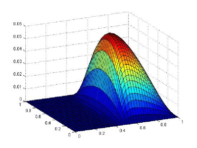
Figure 1: The exact solution $u=\displaystyle\frac{1}{2}x(x-1)y(y-1)(1-tanh(10-20x))$.

Results are presented for uniformly refined meshes. In Tables 1 and 2, $N$ stands for the number of mesh elements, $\eta=\eta_{CF}+\eta_{NC}+\eta_{NC2}+\eta_{J}$, and $Eff=\eta/||u-u_{h}||_{DG,h}$ is the effectivity index. $CV_{error}$ and $CV_{recov}$ are respectively the convergence order in $\sqrt{1/N}$ of the error $||u-u_{h}||_{DG,h}$ and of $||a^{-1/2}(Gu_{h}-a\nabla u)||$, from one line of the table to the following. First of all, it can be observed for $\varepsilon=1E-02$ that the error $||u-u_{h}||_{DG,h}$ converges towards zero at order one and that, in the same time, the superconvergence property of $||a^{-1/2}(Gu_{h}-a\nabla u)||$ is observed. Moreover, as expected by Theorems 3.1 and 3.14 when $\bar{\rho}$ and $\bar{\gamma}$ are superconvergent terms, the proposed estimator is reliable and efficient since the effectivity index remains constant during the refinement process (around 2.00). For $\varepsilon=1E-04$, the same kind of behaviour occurs. Let us nevertheless note that the convergence rate $CV_{error}$ is astonishment high. In fact, the contribution of the jump term $\left(\sum_{e\in{\mathcal{E}}}h_{e}^{-1}\|\mbox{$\big{[}\big{[}u_{h}\big{]}\big{]}$}\|^{2}_{e}\right)^{1/2}$ arising in $||u-u_{h}||_{DG,h}$ is predominant and goes fast towards zero, while the contribution of $|||u-u_{h}|||$ is smaller but converges at order one once the mesh is fine enough.

$N$	$||u-u_{h}||_{DG,h}$	$CV_{error}$	$\eta$	$Eff$	$||a^{-1/2}(Gu_{h}-a\nabla u)||$	$CV_{recov}$
512	2.22E-02		4.47E-02	2.01	4.29E-03
2048	1.13E-02	0.98	2.29E-02	2.02	1.61E-03	1.41
8192	5.58E-03	1.02	1.13E-02	2.02	4.87E-04	1.73
32768	2.77E-03	1.04	5.57E-03	2.01	1.37E-04	1.83
131072	1.38E-03	1.01	2.77E-03	2.01	3.96E-05	1.79

Table 1: Homogeneous case, $\varepsilon=1E-02$, $\gamma=250$, $\gamma_{a,e}=\varepsilon$.

$N$	$||u-u_{h}||_{DG,h}$	$CV_{error}$	$\eta$	$Eff$	$||a^{-1/2}(Gu_{h}-a\nabla u)||$	$CV_{recov}$
512	2.60E+00		2.72E+00	1.05	3.52E-02
2048	1.46E+00	0.82	8.28E-01	1.06	2.17E-02	0.69
8192	5.38E-01	1.44	5.81E-01	1.09	7.97E-03	1.44
32768	1.84E-01	1.54	2.07E-01	1.12	2.40E-03	1.73
131072	6.83E-02	1.43	8.06E-02	1.18	7.14E-04	1.75

Table 2: Homogeneous case, $\varepsilon=1E-04$, $\gamma=250$, $\gamma_{a,e}=\varepsilon$.

5.2 The singular case

We consider here the domain $\Omega=\{-1<x,y<1\}$, which is decomposed into 4 sub-domains $\Omega_{i}$, $i=1,...,4$, with $\Omega_{1}=(0,1)\times(0,1)$, $\Omega_{2}=(-1,0)\times(0,1)$, $\Omega_{3}=(-1,0)\times(-1,0)$ and $\Omega_{4}=(0,1)\times(-1,0)$. Like in subsection 5.1, the reaction coefficient is $\mu=1$, the velocity field $\beta=(1,0)^{\top}$, but the isotropic diffusion tensor is this time no more homogeneous. It is defined by $a_{|\Omega_{i}}=\varepsilon_{i}\,\mathcal{I}$, with $\varepsilon_{2}=\varepsilon_{4}=1$ and $\varepsilon_{1}=\varepsilon_{3}=C>1$ to be specified.

Using the usual polar coordinates $(r,\theta)$ centered at $(0,0)$, the exact solution is chosen to be equal to the singular function $u(x,y)=\eta(r)\,v(x,y)$ with $v(x,y)=r^{\alpha}\phi(\theta)$, where $\alpha\in(0,1)$ and $\phi$ are chosen such that $v$ is harmonic on each sub-domain $\Omega_{i}$, $i=1,..4$, and satisfies the jump conditions :

$$\left[v\right]=0\mbox{ and }\left[a\nabla v.n\right]=0$$

on the interfaces. The function $\eta$ is a $\mathcal{C}^{1}[0,1]$ truncation function used to ensure homogeneous Dirichlet boudary condition on the boundary. Namely, we chose :

$$\eta(r)=\left\{\begin{array}[]{lll}1&\mbox{ for }0\leq r\leq 1/3,\\ (r-2/3)^{2}\,(54r-9)&\mbox{ for }1/3\leq r\leq 2/3,\\ 0&\mbox{ for }r\geq 2/3.\\ \end{array}\right.$$

It is easy to see (see for instance [11]) that $\alpha$ is the root of the transcendental equation

$$\tan\frac{\alpha\,\pi}{4}=\sqrt{\frac{1}{C}},$$

and since $\alpha<1$, this solution has a singular behavior around the point $(0,0)$. Consequently, a local mesh-refinement strategy is used, based on the estimator $\eta_{T}=\eta_{CF,T}+\eta_{NC,T}+\eta_{J,T}$ and the marking process

$$\eta_{T}>0.75\max_{T^{\prime}}\eta_{T^{\prime}},$$

with a standard refinement procedure associated with a limitation on the minimal angle.

Like in [13], we choose first $C=5$. Figure 2 shows some of the meshes obtained during the local refinement process. Moreover, Table 3 displays the corresponding quantitative results. It can be observed that the error goes towards zero as theoretically expected, and that the effectivity index always remains almost constant, which is quite satisfactory and comparable with results from [9, 16] as well as those of the previous test in subsection 5.1. The superconvergence property of $||a^{-1/2}(Gu_{h}-a\nabla u)||$ is once again observed, and the mesh is automatically refined in the vicinity of the singularity as well as in the zone of the mesh where the gradient of $\eta$ is the highest.

Figure 2: Mesh levels 1, 3 and 5, singular solution for $C=5$.

$N$	$||u-u_{h}||_{DG,h}$	$CV_{error}$	$\eta$	$Eff$	$||a^{-1/2}(Gu_{h}-a\nabla u)||$	$CV_{recov}$
128	1.26E+00		3.09E+00	2.44	1.14E+00
468	4.72E-01	1.51	1.25E+00	2.65	4.55E-01	1.41
2016	2.14E-01	1.08	5.74E-01	2.68	1.36E-01	1.65
9068	1.01E-01	1.00	2.81E-01	2.76	4.68E-02	1.41

Table 3: Homogeneous case, $C=5$, $\gamma=50$, $\gamma_{a,e}=1$.

Secondly, we consider a stronger singularity by choosing $C=100$. Figure 3 shows some of the meshes obtained during the local refinement process, and Table 4 displays the corresponding quantitative results. The results are very similar to the ones obtained for $C=5$. Like in [13], the refinement process is faster around the interfaces (and the origin). The effectivity index slightly increases while remaining constant during all the refinement process, and the superconvergence property of $||a^{-1/2}(Gu_{h}-a\nabla u)||$ is observed.

Figure 3: Mesh levels 1, 3 and 15, singular solution for $C=100$.

$N$	$||u-u_{h}||_{DG,h}$	$CV_{error}$	$\eta$	$Eff$	$||a^{-1/2}(Gu_{h}-a\nabla u)||$	$CV_{recov}$
128	1.56E+00		6.34E+00	4.05	2.92E+00
504	7.25E-01	1.12	3.65E+00	5.03	7.99E-01	1.89
2208	4.48E-01	0.65	1.95E+00	4.35	3.81E-01	1.00
7716	2.44E-01	0.97	1.09E+00	4.46	1.60E-01	1.38

Table 4: Homogeneous case, $C=100$, $\gamma=500$, $\gamma_{a,e}=1$.

5.3 The boundary-layer case

We now consider the domain $\Omega=\{0<x,y<1\}$, with the reaction coefficient $\mu=0$ and the velocity field $\beta=(1,0)^{\top}$. The homogeneous isotropic diffusion tensor is defined by $a=\varepsilon\,\mathcal{I}$, with $\varepsilon=1E-02$. The source term $f$ is chosen accordingly so that $u=10y(1-y)x(e^{-x}-e^{-1+\frac{x-1}{\alpha}})$ is the exact solution (see Figure 4), with $\alpha=1E-03$ in order to generate a strong boundary layer. Here, the same refinement procedure than in section 5.2 is used.

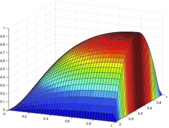
Figure 4: The exact solution $u=10y(1-y)x(e^{-x}-e^{-1+\frac{x-1}{\alpha}})$, with $\alpha=1E-03$.

Figure 5 shows some of the meshes obtained during the local refinement process. Moreover, Table 5 displays the corresponding quantitative results. Provided that the boundary layer mesh resolution is sufficient, the same behaviours than in the previous tests can also be observed : the error goes towards zero as theoretically expected, the effectivity index remains almost constant, the superconvergence property of $||a^{-1/2}(Gu_{h}-a\nabla u)||$ occurs, and the mesh is automatically refined around the boundary layer.

Figure 5: Mesh levels 1, 5 and 16, non homogeneous boundary-layer case.

$N$	$||u-u_{h}||_{DG,h}$	$CV_{error}$	$\eta$	$Eff$	$||a^{-1/2}(Gu_{h}-a\nabla u)||$	$CV_{recov}$
156	5.90E+00		9.11E+00	1.54	1.46E+00
766	1.32E+00	1.88	2.52E+00	1.90	8.84E-01	0.63
3033	5.76E-01	1.21	1.24E+00	2.16	3.67E-01	1.27
12881	2.53E-01	1.13	5.34E-01	2.10	1.19E-01	1.58
50496	1.26E-01	1.02	2.66E-01	2.11	5.02E-02	1.26

Table 5: Boundary-layer case, $\varepsilon=1E-02$, $\gamma=250$, $\gamma_{a,e}=\varepsilon$.

References

• [1] M. Ainsworth. A posteriori error estimation for discontinuous Galerkin finite element approximation. SIAM J. Numer. Anal., 45(4):1777–1798 (electronic), 2007.
• [2] M. Ainsworth and J. Oden. A posteriori error estimation in finite element analysis. John Wiley and Sons, 2000.
• [3] D. G. Arnold, F. Brezzi, B. Cockburn, and L. D. Marini. Unified analysis of discontinuous Galerkin methods for elliptic problems. SIAM J. Numer. Anal., 39:1749–1779, 2001.
• [4] I. Babuška and T. Strouboulis. The finite element methods and its reliability. Clarendon Press, Oxford.
• [5] R. Becker, P. Hansbo, and M. G. Larson. Energy norm a posteriori error estimation for discontinuous Galerkin methods. Comput. Meth. Appl. Mech. Engrg., 192:723–733, 2003.
• [6] D. Braess and J. Schöberl. Equilibrated residual error estimator for edge elements. Math. Comp., 77(262):651–672, 2008.
• [7] S. C. Brenner and L. R. Scott. The Mathematical Theory of Finite Element Methods. Springer Verlag, New York, 1994.
• [8] P. G. Ciarlet. The finite element method for elliptic problems. North-Holland, Amsterdam, 1978.
• [9] S. Cochez-Dhondt and S. Nicaise. Equilibrated error estimators for discontinuous Galerkin methods. Numer. Meth. PDE, 24:1236–1252, 2008.
• [10] B. Cockburn, G. E. Karniadakis, and C.-W. Shu. The development of discontinuous Galerkin methods, volume 11 of Lect. Notes Comput. Sci. Eng. Springer Verlag, Berlin, 2000.
• [11] M. Costabel, M. Dauge, and S. Nicaise. Singularities of Maxwell interface problems. RAIRO Modél. Math. Anal. Numér., 33:627–649, 1999.
• [12] E. Creusé and S. Nicaise. Anisotropic a posteriori error estimation for the mixed discontinuous Galerkin approximation of the Stokes problem. Numer. Meth. PDE, 22:449–483, 2006.
• [13] E. Creusé and S. Nicaise. A posteriori error estimator based on gradient recovery by averaging for discontinuous Galerkin methods J. Comput. Appl. Math., 234, 2903-2915, 2010.
• [14] E. Dari, R. Durán, C. Padra, and V. Vampa. A posteriori error estimators for nonconforming finite element methods. M2AN, 30:385–400, 1996.
• [15] A. Ern, S. Nicaise, and M. Vohralík. An accurate $\mathbb{H}({\rm div})$ flux reconstruction for discontinuous Galerkin approximations of elliptic problems. C. R. Math. Acad. Sci. Paris, 345(12):709–712, 2007.
• [16] A. Ern, A. F. Stephansen, and M. Vohralík. Guaranteed and robust discontinuous galerkin a posteriori error estimates for convection-diffusion-reaction problems. J. Comput. Appl. Math., 234:114 –130, 2010.
• [17] A. Ern, A. F. Stephansen, and P. Zunino. A discontinuous Galerkin method with weighted averages for advection–diffusion equations with locally small and anisotropic diffusivity. IMA J. Numer. Anal., 29(2):235–256, 2009.
• [18] F. Fierro and A. Veeser. A posteriori error estimators, gradient recovery by averaging, and superconvergence. Numer. Math., 103(2):267–298, 2006.
• [19] W. Hoffmann, A. H. Schatz, L. B. Wahlbin, and G. Wittum. Asymptotically exact a posteriori estimators for the pointwise gradient error on each element in irregular meshes. I. A smooth problem and globally quasi-uniform meshes. Math. Comp., 70(235):897–909 (electronic), 2001.
• [20] P. Houston, I. Perugia, and D. Schötzau. Energy norm a posteriori error estimation for mixed discontinuous Galerkin approximations of the Maxwell operator. Comput. Meth. Appl. Mech. Engrg., 194:499–510, 2005.
• [21] P. Houston, I. Perugia, and D. Schötzau. A posteriori error estimation for discontinuous Galerkin discretization of the H(curl)-ellipic partial differential operator. IMA J. Numer. Analysis, 27:122–150, 2007.
• [22] O. A. Karakashian and F. Pascal. A posteriori error estimates for a discontinuous Galerkin approximation of second-order problems. SIAM J. Numer. Anal., 41:2374–2399, 2003.
• [23] P. Ladevèze and D. Leguillon. Error estimate procedure in the finite element method and applications. SIAM J. Numer. Anal., 20:485–509, 1983.
• [24] R. Lazarov, S. Repin, and S. Tomar. Functional a posteriori error estimates for discontinuous galerkin approximations of elliptic problems. Report 2006-40, Ricam, Austria, 2006.
• [25] R. Luce and B. Wohlmuth. A local a posteriori error estimator based on equilibrated fluxes. SIAM J. Numer. Anal., 42:1394–1414, 2004.
• [26] P. Monk. A posteriori error indicators for Maxwell’s equations. J. Comput. Appl. Math., 100:73–190, 1998.
• [27] P. Monk. Finite element methods for Maxwell’s equations. Numerical Mathematics and Scientific Computation. Oxford University Press, 2003.
• [28] P. Neittaanmaäki and S. Repin. Reliable methods for computer simulation: error control and a posteriori error estimates., volume 33 of Studies in Mathematics and its applications. Elsevier, Amsterdam, 2004.
• [29] S. Nicaise, K. Witowski, and B. I. Wohlmuth. An a posteriori error estimator for the Lamé equation based on equilibrated fluxes. IMA J. Numer. Anal., 28(2):331–353, 2008.
• [30] B. Rivière and M. Wheeler. A posteriori error estimates for a discontinuous Galerkin method applied to elliptic problems. Comput. Math. Appl., 46(1):141–163, 2003.
• [31] A. H. Schatz and L. B. Wahlbin. Asymptotically exact a posteriori estimators for the pointwise gradient error on each element in irregular meshes. II. The piecewise linear case. Math. Comp., 73(246):517–523 (electronic), 2004.
• [32] A. Schmidt and K. G. Siebert. Design of adaptive finite element software, volume 42 of Lecture Notes in Computational Science and Engineering. Springer-Verlag, Berlin, 2005. The finite element toolbox ALBERTA, With 1 CD-ROM (Unix/Linux).
• [33] D. Schötzau and L. Zhu. A robust a-posteriori error estimator for discontinuous Galerkin methods for convection-diffusion equations. Appl. Numer. Math., 59(9):2236–2255, 2009.
• [34] S. Sun and M. F. Wheeler. $L^{2}(H^{1})$ norm a posteriori error estimation for discontinuous Galerkin approximations of reactive transport problems. J. Sci. Comput., 22-23:501–530, 2005.
• [35] R. Verfürth. A review of a posteriori error estimation and adaptive mesh-refinement thecniques. Wiley–Teubner Series Advances in Numerical Mathematics. Wiley–Teubner, Chichester, Stuttgart, 1996.
• [36] R. Verfürth. Robust a posteriori error estimates for stationary convection-diffusion equations. SIAM J. Numer. Anal., 43(4):1766–1782 (electronic), 2005.
• [37] M. Vohralík. A posteriori error estimates for lowest-order mixed finite element discretizations of convection-diffusion-reaction equations. SIAM J. Numer. Anal., 45(4):1570–1599 (electronic), 2007.
• [38] M. Vohralík. Residual flux-based a posteriori error estimates for finite volume and related locally conservative methods. Numer. Math., 111(1):121–158, 2008.
• [39] Z. Zhang. A posteriori error estimates on irregular grids based on gradient recovery. Adv. Comput. Math., 15(1-4):363–374 (2002), 2001.