Compressibility of graphene

Abstract

We develop a theory for the compressibility and quantum capacitance of disordered monolayer and bilayer graphene including the full hyperbolic band structure and band gap in the latter case. We include the effects of disorder in our theory, which are of particular importance at the carrier densities near the Dirac point. We account for this disorder statistically using two different averaging procedures: first via averaging over the density of carriers directly, and then via averaging in the density of states to produce an effective density of carriers. We also compare the results of these two models with experimental data, and to do this we introduce a model for inter-layer screening which predicts the size of the band gap between the low-energy conduction and valence bands for arbitary gate potentials applied to both layers of bilayer graphene. We find that both models for disorder give qualitatively correct results for gapless systems, but when there is a band gap in the low-energy band structure, the density of states averaging is incorrect and disagrees with the experimental data.

I Introduction

Recently, graphene has become a highly-studied electronic system with many potential uses in electronic devices, optics, and sensing applications.abergel-advphys While significant theoretical effort has been concentrated on the transport propertiesdassarma-rmp (such as the minimal conductivity, localization effects, and signatures of relativistic behavior of the charge carriers), bulk thermodynamic quantities such as the compressibility of the electron liquid in monolayer and bilayer graphene have also received substantial attention. The compressibility is an important quantity because it is possible to extract information about the electron-electron interactions and correlations directly from these measurements, and to gain information about fundamental physical quantities such as the pair correlation function. The quantum capacitancejohn-jap96 ; fang-apl91 is also an important quantity in the context of device design and fundamental understanding of the graphene system. In fact, the compressibility is often inferred from the measurement of quantum capacitance.

Experimentsmartin-natphys4 have shown that the contribution to the compressibility of monolayer graphene from electron-electron interactions is small (amounting to a $10-15\%$ renormalization of the effective Fermi velocity). This was explained within the Hartree–Fock approximation.hwang-prl99 Capacitance measurements of bilayer graphene have also been carried out recently,young-arXiv ; henriksen-prb82 and they purport to show data which indicates that the quadratic approximation of the band structure of this material does not produce the correct predictions for the quantum capacitance of the graphene sheet. Other measurements which claim to access the quantum capacitance directly have shown similar behavior.xia-natnano4

Theoretical work has been published which considers the compressibility of monolayerhwang-prl99 and bilayerkusminskiy-prl100 graphene at the Hartree-Fock level and in the random phase approxmationborghi-prb82 (RPA). They find that interactions are more important in the bilayer system (due to the finite density of states at charge-neutrality), but that in the RPA the contributions from exchange and correlation almost cancel each other out leaving a small positive compressibility at all densities. A consensus has developed that many-body corrections to the compressibility in graphene are at most of the order of 10% at reasonable carrier densities.sensarma-unpub

In this article we discuss theoretically the compressibility of monolayer and bilayer graphene, and specifically employ the four-band model of bilayer graphene (which generates the non-quadratic band structure). We will highlight the similarities and differences between this model and the linear and quadratic cases, and take into account the possiblility of a gap at the charge-neutrality point. We find that the non-quadratic band structure significantly affects the theoretical predictions for the compressibility and brings them into qualitative and semi-quantitative agreement with experimental findings. We also include disorder in the form of electron–hole puddles created by charged impurities in the vicinity of the graphene. We discuss two different procedures for including this effect statistically and determine the validity of each model by comparing with experimental data. The first assumes that the disorder creates a spatial variation in the density of carriers which can be modelled by averaging a physical quantity such as compressiblity over a range of densities. The second model assumes that disorder affects the local density of states which can be averaged to give an effective bulk density of carriers which can then be used to compute the physical quantities of interest. We find that for gapless graphenes, inclusion of disorder by either method predicts qualitatively correct results in agreement with experiments, but when a gap is opened, the stage at which the averaging is done makes a critical difference.

Therefore, we have dual complementary theoretical goals in this work. Our primary goal is to develop an accurate (and essentially approximation-free) theory for the graphene compressibility within the non-interacting electron model which incorporates all aspects of the realistic band structure as well as effects of the disorder within reasonable and physically motivated approximations. Our secondary goal is to compare our theory closely and transparently with the existing experimental data on the compressibility of bilayer graphene so as to obtain some well-informed conclusions about the possible role of many-body exchange-correlation effects, which have recently been studied the the literaturekusminskiy-prl100 ; borghi-prb82 ; sensarma-unpub but which are beyond the scope of the current work. We believe that an accurate calculation of graphene compressibility within the free electron theory neglecting all interaction effects is warranted for (at least) three reasons: (i) without an accurate one-electron theory, quantitative conclusions regarding many-body effects are not useful; (ii) many-body theory is, by definition, approximate and, as such, subject to doubts; (iii) many-body corrections to graphene compressibility are claimed to be small with considerable cancellation between exchange and correlation effectsborghi-prb82 . In comparing our theoretical results with the experimental data, we find that the inclusion of disorder effects in the theory is of qualitative importance, particularly at low carrier densities near the charge-neutral Dirac point (where the many-body effects are expected to be largest). The inclusion of disorder through two alternative physical approximations and the eventual validation of one of the models of disorder by comparing with the existing experimental data is an important accomplishment of our theory.

To outline the structure of this article, we begin in the remainder of this section by giving details of the band structures of the three types of graphene which we consider. In Section II we introduce a model for determining the band gap in bilayer graphene with arbitrary gate potentials applied to both layers. Then, in Section III we describe the calculation of $K=\frac{d\mu}{dn}$ in the homogeneous (non-disordered) situation (where $\mu$ and $n$ are the chemical potential and carrier density respectively) for each of these three cases and discuss the main features of this quantity in relation to the quantum capacitance and compressibility. In Section IV we introduce the two models for the inclusion of disorder and present the fundamental theoretical results for each. Then, in Section V we compare the predictions of our theory to experminental data given by capacitance measurements of bilayer graphene which include the quantum capacitance of the 2D electron gas. Finally, in Section VI we summarize our results and give some general discussion of our findings.

In the following, we discuss three different models for the single-particle dispersion of graphene which we denote by $E_{k}$. We shall refer to these three cases as linear, quadratic, and hyperbolic graphene to distinguish them. For the monolayer, we have $E^{l}_{k}=\hbar v_{F}k$ as is well-known, and we indicate all quantities which follow from this dispersion by attaching a superscript ‘$l$’ as we have here. For bilayer graphene, there are two commonly-used approximations for the low-energy single-particle dispersion. The simplest is the quadratic approximation $E^{q}_{k}=\hbar^{2}v_{F}^{2}k^{2}/\gamma_{1}=\hbar^{2}k^{2}/(2m)$ where $\gamma_{1}$ is the inter-layer hopping parameter from the tight-binding theory and $m=\gamma_{1}/(2v_{F}^{2})$ is the effective mass of the electrons. This dispersion comes from a low-energy effective theory of bilayer graphenemccann-prl96 which essentially discards the two split bands and confines electrons to those lattice sites not involved in the inter-layer coupling. This quadratic bilayer dispersion is assumed to hold for low carrier densities, i.e. at low Fermi energy.dassarma-rmp Alternatively, the full tight-binding theorymccann-prb74 yields the single-particle dispersion

$$E^{h}_{k}=\pm\sqrt{\frac{\gamma_{1}^{2}}{2}+\frac{u^{2}}{4}+\hbar^{2}v_{F}^{2}k^{2}-\sqrt{\frac{\gamma_{1}^{4}}{4}+\hbar^{2}v_{F}^{2}k^{2}(\gamma_{1}^{2}+u^{2})}}$$ (1)

for the low-energy bands, which is illustrated for the conduction band in Fig. 1. This dispersion allows for the inclusion of a band gap parameterized by the energy $u$ which corresponds to the potential energy difference between the two layers. The ‘sombrero’ shape of the dispersion implies that the minimum gap is found at wave vector $k^{\ast}=\frac{u}{2\hbar v_{F}}\sqrt{\frac{2\gamma_{1}^{2}+u^{2}}{\gamma_{1}^{2}+u^{2}}}$ and the energy of the minimum is therefore $E^{\ast}=\frac{\gamma_{1}u}{2\sqrt{\gamma_{1}^{2}+u^{2}}}$. This non-monotonic dispersion relation leads to some important features in the Fermi surface at low density. For medium and high density regimes (when $k_{F}>\frac{u}{\hbar v_{F}}$), the Fermi wave vector is given by $k_{F}=\sqrt{\pi n}$ and the Fermi surface is disc-shaped. However, if $\sqrt{\pi n}<\frac{u}{\hbar v_{F}}$ (as sketched in Fig. 1) then the Fermi energy is in the ‘sombrero’ region and the Fermi surface is ring-shapedstauber-prb75 with $k_{F-}<k<k_{F+}$ and

$$k_{F\pm}=\frac{1}{2\hbar v_{F}}\sqrt{\frac{\pi^{2}\hbar^{4}v_{F}^{4}n^{2}+\gamma_{1}^{2}u^{2}}{\gamma_{1}^{2}+u^{2}}+u^{2}\pm 2\pi\hbar^{2}v_{F}^{2}n}.$$ (2)

Clearly these characteristic features of the full hyperbolic bilayer band dispersion are lost in the linear (“high-energy”) and quadratic (“low-energy”) approximations often adopted in the literature for simplicity.

Figure 1: Sketch of the ‘sombrero’ dispersion in hyperbolic graphene with $u>0$. The depth of the minimum is exagerrated for the purposes of illustration. The various wave vectors and energies that are labeled are defined in the text.

The parameter $u$ can be treated in two ways. Initially (and in Section IV), we consider it to be a phenomenological parameter which can be chosen arbitrarily to represent a finite gap at charge-neutrality. However, in order to accurately compare our theory with experiment we must determine a method of relating $u$ to the external gate potentials. To do this accurately, the screening of the external field by the charge on the two layers of bilayer graphene must be taken into account, and we describe this process in Section II.

II Inter-layer screening

In order to make an accurate comparison with experimental data, we must properly map the gate voltages applied in experiment to the parameters $n$ and $u$ which appear in our theory. We assume the situation sketched in Fig. 2(a). The density is easily computed via elementary considerations to be $n=\epsilon_{0}\left(V_{b}\epsilon_{b}/d_{b}+V_{t}\epsilon_{t}/d_{t}\right)/e$ where $V$ is the voltage applied to a gate, $d$ is the width of the gate layer, $\epsilon$ is the dielectric constant of the gate, and the subscript $b$ and $t$ respectively denote the bottom and top gates. The zeroeth-order approximation for the on-site potential $u$ is to say that the electric field created by the gates directly gives the electric field $E$ in the graphene. The potential is then $u_{t,b}=\pm eEd/2$. However, this approximation does not take into account the screening effect of the charge on the two graphene layers. Previously, various authors have investigated this problem and shown that screening reduces the size of the gap mccann-prb74 ; min-prb75 ; castro-prl99 . We extend this work to the case where the total density is finite and gates are present both above and below the graphene layer.

Since the screening depends only on the electric field created by the gates and the charge densities on the two layers, it is independent of the disorder caused by charged impurities. Both the screening and the disorder effects are determined by the net carrier density, and both leave this quantity unchanged. Therefore, we can use the following analysis to set the size of the gap for any given set of external conditions, and use the resulting band structure to calculate the effect of disorder for that situation. This is allowed because neither disorder nor the screening induces any extra charge in the graphene. Additionally, we will assume in Section IV that the disorder potential is the same in both layers meaning that it does not induce any inter-layer scattering and therefore leaves the net carrier density in each layer unchanged.

Figure 2: (a) The geometry of the screening problem. The external field $E_{\text{ext}}=(E_{b}+E_{t})/2$ is screened by redistribution of the charge density $n=n_{b}+n_{t}$ between the two layers of the graphene. (b) The screened gap $u$ as a function of the bare gap $u_{\text{ext}}$ for various densities. (c) The screened gap as a function of the top gate voltage for various fixed back gate voltages and the experimental parameters used in the experiments of Young et al.young-arXiv ; exppar Back gate voltages are quoted in Volts.

According to Gauss’ law, the electric field directed away from an infinite-sized, positively charged sheet is $E=qn/2\epsilon_{0}$, where $q=-|e|$ is the charge of the carriers on the sheet. Hence, we can write the internal field (i.e. the field between the graphene layers) as

$$E=E_{\mathrm{ext}}+\frac{e}{2\epsilon_{0}}(n_{t}-n_{b}).$$ (3)

That this internal field is different from the external one causes the free charge on the two layers to rearrange, which in turn further modifies the internal field. A self-consistent procedure can be constructed to find the final solution for the layer charge densities and the internal electric field. This additional field causes an additional Hartree energy of $u_{t}-u_{b}=edE$ to be added to the on-site potential in the original Hamiltonian. This modified on-site potential will be smaller than in the unscreened case, and therefore the gap will also be smaller.

We implement this procedure for a given pair of gate voltages $V_{b}$ and $V_{t}$ as follows. The first step is to compute the unscreened on-site potential in the two layers, which is given by the expression above with $n_{t}=n_{b}$ so that $E=E_{\mathrm{ext}}$. This gives $u_{\mathrm{ext}}=edE_{\mathrm{ext}}=ed(V_{b}/d_{b}-V_{t}/d_{t})/2$. We assume that the potential is symmetrical so that $u_{t}=u/2$ and $u_{b}=-u/2$. This determines the single-particle Hamiltonian, from which we can compute the wave functions. The layer density is then found by summing the wave function weight in each layer:

$$n_{t}=\sum_{\mathrm{states}}\left(|\phi_{At}|^{2}+|\phi_{Bt}|^{2}\right)$$

where $A$ and $B$ label the two inequivalent lattice sites in each layer. The sum runs over all valley, spin and wave vector states. A similar expression is given for the lower layer by substituting $t\to b$ throughout. Computing these densities gives all the information required to evaluate the internal electric field, from which we can find the modified on-site potentials via Eq. (3). These potentials are then used to calculate the modified layer densities, and this cycle is repeated until convergence is reached.

Figure 2(b) shows the screened gap as a function of the external gap for various density of carriers. The density plays a role because the more free carriers there are, the more effectively the external field can be screened and the smaller the screened gap is. This is shown in the figure because the magnitude of the gap for $|n|=5\times 10^{12}\mathrm{cm}^{-2}$ is always smaller than that for $|n|=1\times 10^{12}\mathrm{cm}^{-2}$. Figure 2(c) shows the screened gap as a function of top gate voltage assuming that the back gate voltage is fixed. We have used the parameters from the experiments by Young et al.young-arXiv ; exppar . The peak in each trace is caused by the approach of the system to charge neutrality where there are no excess carriers and hence the external electric field is unscreened. At this point, the screened gap is equal to the bare gap. When there is a finite density of excess carriers, the external field is screened and the gap reduced accordingly. As the back gate voltage is changed, the position of the charge neutrality point shifts and the size of the gap at charge neutrality increases. Inclusion of inter-layer screening turns out to be important for understanding the experimental data.

III Calculation of $\frac{d\mu}{dn}$

In this section, we describe the calculation of $\frac{d\mu}{dn}$ for the homogeneous (non-disordered) system. The results derived here will be used later to compute the same quantity for a disordered system. The single-particle dispersions $E_{k}$ of monolayer and bilayer graphene are well known (as discussed in Section I). From these relations, we can compute the total kinetic energy for excess charge carriers by summing the energy of carriers in filled states: $\mathcal{E}=\sum_{\text{states}}E_{k}n_{F}(k)$ where $n_{F}(k)$ is the Fermi distribution function with wave vector $k=|\boldsymbol{\mathrm{k}}|$. Then, the chemical potential is defined to be the change in energy with the addition of a particle, which is expressed as $\mu=\frac{1}{\mathcal{A}}\frac{d\mathcal{E}}{dn}$ where $n$ is the carrier density and $\mathcal{A}$ is the area of the graphene flake. From this we can compute $K=\frac{d\mu}{dn}$, and the quantum capacitance $C_{Q}$ and compressibility $\kappa$ are then linked to this quantity via

$$C_{Q}=\mathcal{A}e^{2}\frac{dn}{d\mu},\qquad\kappa^{-1}=n^{2}\frac{d\mu}{dn}.$$ (4)

The linear and quadratic band structures lead straightforwardly to the following expressions

$$K^{l}=\frac{\hbar v_{F}\sqrt{\pi}}{2\sqrt{n}},\quad\text{and}\quad K^{q}=\frac{\hbar^{2}v_{F}^{2}\pi}{\gamma_{1}}.$$

The linear dispersion leads to a square-root divergence at zero density while the quadratic version gives a constant for all densities. It is possible to obtain an analytical expression for $K^{h}$ in various limits and we present them in the Appendix. Here, we describe a process for writing down the answer. Starting from the expression for the total energy, the sum is evaluated by transforming to an integral over $k$. The indefinite integral in question is given by

$$I(k)=\frac{2\mathcal{A}}{\pi}\int kE_{k}^{h}\,dk.$$ (5)

To find the total energy, we write the sum over states discussed above as an integral over the wave vector. Then, evaluation of the Fermi function naturally leads to an expression containing $I(k)$ at the limiting values of the wave vector for the specific value of the density:

$$\mathcal{E}=\frac{2\mathcal{A}}{\pi}\int_{0}^{\infty}kE_{k}^{h}n_{F}(k)\,dk=I(k=k_{F_{+}})-I(k=k_{F_{-}}).$$

The chemical potential can be calculated by transforming the derivative into one for the limiting $k$:

$$\mu=\frac{1}{\mathcal{A}}\frac{d\mathcal{E}}{dn}=\frac{1}{\mathcal{A}}\frac{dk_{F_{+}}}{dn}\frac{dI(k_{F_{+}})}{dk_{F_{+}}}-\frac{1}{\mathcal{A}}\frac{dk_{F_{-}}}{dn}\frac{dI(k_{F_{-}})}{dk_{F_{-}}}.$$

However, it is clear from the fundamental theorem of calculus and the definition of $I$ that $dI/dk=2\mathcal{A}kE_{k}/\pi$ so that the second derivative is straightforward to calculate and we have

$$K^{h}=\frac{2}{\mathcal{\pi}}\bigg{\{}\frac{d^{2}k_{F_{+}}}{dn^{2}}k_{+}E_{k_{F_{+}}}-\frac{d^{2}k_{F_{-}}}{dn^{2}}k_{F_{-}}E_{k_{F_{-}}}\\ +\left(\frac{dk_{F_{+}}}{dn}\right)^{2}\left(E_{k_{F_{+}}}+k_{F_{+}}\frac{dE_{k_{F_{+}}}}{dk_{F_{+}}}\right)\\ -\left(\frac{dk_{F_{-}}}{dn}\right)^{2}\left(E_{k_{F_{-}}}+k_{F_{-}}\frac{dE_{k_{F_{-}}}}{dk_{F_{-}}}\right)\bigg{\}}.$$ (6)

The remaining derivatives are simple to compute from Eqs. (1) and (2). As described previously, when $|E_{F}|<u/2$ the values of $k_{\pm}$ are given by Eq. (2). When $|E_{F}|>u/2$ (which is trivially the case for $u=0$) then $k_{-}=0$ and $k_{+}=\sqrt{\pi n}$ and only the first two terms contribute to $K^{h}$. This is the central result of this section, but in the Appendix we have evaluated this expression for various limiting cases.

The three versions of $K$ are plotted in Figure 3(a) where the density is assumed to be a tunable external parameter and the gap is fixed. In the limit of small $n$, the gapless hyperbolic band structure is roughly quadratic and so $K^{h}$ is very close to $K^{q}$. However, the linearity of the hyperbolic dispersion quickly asserts itself to reduce the size of $K^{h}$ until, at high density, it approaches the value of linear graphene. Thus $K^{h}$ in the ungapped regime interpolates between these two limiting cases as one expects. We also show $K^{h}$ for the gapped case (red or light gray line) where we take $u=50\mathrm{meV}$. When the density is high and the Fermi energy is well above the gap region, $K^{h}$ tends to the same functional form as for the ungapped scenario. However, when the density is low, $K^{h}$ goes to zero for any finite $u$. The large reduction in $K^{h}$ by the gap will be an important feature for the comparison with experiment. In Figure 3(b) we show the $K^{h}$ at low carrier density for several different values of the gap. One immediately notices a discontinuity when $n=u/(\hbar v_{F})$ which is caused by the change in topology of the Fermi surface from a ring to a disc. When a gap is present, there is also a $\delta$-function divergence at $n=0$ (not shown in the plots) caused by the step in the chemical potential as the Fermi energy goes from the valence band to the conduction band. The prefactor of this divergence is the size of the gap so that it is not present when $u=0$.

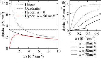
Figure 3: (a) The inverse density of states, $K=\frac{d\mu}{dn}$ for linear, quadratic, gapless hyperbolic and gapped hyperbolic ($u=50\mathrm{meV}$) dispersions. (b) $K$ for different gap sizes at low carrier density.

IV Models for disorder

We now discuss the effects of disorder caused by electron-hole puddles which are formed by charged impurities in the environment.martin-natphys4 ; rossi-prl101 We will describe two inequivalent methods of averaging over disorder and highlight the differences between them. In what follows, we must be careful to distinguish global (averaged) quantities from their local counterparts. Therefore, we use an overbar to denote a quantity which has been averaged over disorder and which is therefore global. We start by assuming that charged impurities (which may be located in the substrate or near the graphene) create a local electrostatic potential which fluctuates randomly across the surface of the graphene sheet. In the case of the bilayer, we assume that this potential is felt equally by both layers. We then make the transition from the spatial variation of the potential to an average by assuming that the value of this potential at any given point can be described by a statistical distribution.hwang-prb82 This distribution can then be used to average some pertinent quantity to obtain the bulk result for the disordered system. But it is not clear a priori what the optimum method of performing this average is. In order to discuss this question, we use two different methods and (in the next section) compare the results of each to experimental data.

The first model assumes that the disorder potential directly affects the density of carriers in the graphene so that the density is distributed according to a Gaussian distribution $P$ parameterized by width $\nu$

$$P(n)=\frac{1}{\nu\sqrt{2\pi}}\exp\left(-\frac{n^{2}}{2\nu^{2}}\right).$$

Then, the overall value of $\overline{K}=\overline{\frac{d\mu}{dn}}$ can be found by evaluating the convolution of the homogeneous (non-disordered) $K$ with this distribution:

$$\overline{\frac{d\mu}{dn}}=\int_{-\infty}^{\infty}\frac{d\mu(n-n^{\prime})}{d(n-n^{\prime})}P(n^{\prime})dn^{\prime}.$$ (7)

This has the effect of broadening any sharp features in the homogenous $K$, such as the $\delta$-function at $n=0$ in a gapped system or the step associated with the change in topology of the Fermi surface in the hyperbolic band. Specifically, evaluating this convolution gives the following contribution to $\overline{K}$ for the hyperbolic band from the $\delta$-function:

$$\frac{u\gamma_{1}}{\sqrt{u^{2}+\gamma_{1}^{2}}}\frac{\exp\left(-n^{2}/2(\delta n)^{2}\right)}{\delta n\sqrt{2\pi}}$$

so that this spike is broadened into a peak where the height is determined by the size of the effective gap $2E^{\ast}$. This model corresponds to that taken in Ref. henriksen-prb82, , except that our theory includes the inter-layer screening which reduces the gap size.

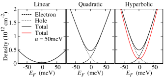
Figure 4: Electron, hole and total carrier densities for linear, quadratic and hyperbolic graphene for $s=20\mathrm{meV}$.

The second model assumes that the disorder potential introduces variation in the density of states (DoS). The potential itself is assumed to follow a Gaussian distribution $P(V)$ parameterized by width $s$, and therefore the disordered DoS is given byhwang-prb82

$$D(E)=\int_{-\infty}^{\infty}D_{0}(E-V)P(V)dV$$ (8)

where $D_{0}(E)$ is the homogeneous (non-disordered) DoS. This modified DoS then gives the zero-temperature electron density by integrating over energy so that

$$\overline{n}(E_{F})=\int_{-\infty}^{\infty}D(E)\Theta(E_{F}-E)dE$$ (9)

where $E_{F}$ is the global Fermi energy and $\Theta(x)$ is the Heaviside step function. A similar expression exists for the density of holes. This density is assumed to hold throughout the graphene so that the averaged density can now be used to evaluate $\overline{K}=\frac{d\mu(\overline{n})}{dn}$. Since we assume that the disorder does not induce any additional charge in the 2D system, the net carrier density $n^{e}-n^{h}$ is conserved. Therefore, to compute the effective Fermi energy $\overline{E_{F}}$ in the presence of disorder we solve the equation $\overline{n}^{e}(\overline{E_{F}})-\overline{n}^{h}(\overline{E_{F}})=n_{0}^{e}(E_{F})-n_{0}^{h}(E_{F})$ for $\overline{E_{F}}$. However, the total carrier density $n^{e}+n^{h}$ is not conserved, and the primary effect of disorder in this model is to introduce a finite total density for any finite amount of charged impurities.

The integrals in Eqs. (8) and (9) can be computed analytically for the linear and quadratic bands if we assume that $P(V)$ is a Gaussian distribution. They are

$$\overline{n}^{l}=\frac{1}{\pi\hbar^{2}v_{F}^{2}}\left[\frac{E_{F}^{2}+s^{2}}{2}\mathrm{erfc}(\mp y)\pm\frac{E_{F}s}{\sqrt{2\pi}}e^{-y^{2}}\right]$$

and

$$\overline{n}^{q}=\frac{\gamma_{1}}{2\pi\hbar^{2}v_{F}^{2}}\left[s\sqrt{\tfrac{2}{\pi}}e^{-y^{2}}\pm E_{F}\mathrm{erfc}(\mp y)\right].$$

where the upper sign corresponds to the electron density and the lower sign to the hole density, $\mathrm{erfc}$ is the complementary error function, and $y=E_{F}/(\sqrt{2}s)$ with $s$ the standard deviation of the distribution of the disorder potential. We see that the effect of disorder is to introduce a tail in the electron density which extends into the conduction band, the size of which increases with increasing disorder strength. In the hyperbolic case, the integrals in Eqs. (8) and (9) cannot be evaluated analytically, so a numerical comparison must be done with the other two cases. The expressions which must be computed for the hyperbolic band are

$$n^{he}=\frac{1}{s\sqrt{2\pi}}\frac{1}{\pi\hbar^{2}v_{F}^{2}}\int_{-\infty}^{E_{F}}dE\Bigg{[}\int_{-\infty}^{E-E^{\ast}}dV(E-V)\left[2+\mathcal{F}(E-V)\right]e^{-V^{2}/(2s^{2})}\\ -\int_{E-\frac{u}{2}}^{E-E^{\ast}}dV\,(E-V)\left[2-\mathcal{F}(E-V)\right]e^{-V^{2}/(2s^{2})}\Bigg{]}$$

and

$$n^{hh}=\frac{1}{s\sqrt{2\pi}}\frac{1}{\pi\hbar^{2}v_{F}^{2}}\int_{E_{F}}^{\infty}dE\bigg{[}-\int_{E+E^{\ast}}^{\infty}dV(E-V)\left[2+\mathcal{F}(E-V)\right]e^{-V^{2}/(2s^{2})}\\ +\int_{E+E^{\ast}}^{E+\frac{u}{2}}(E-V)\left[2-\mathcal{F}(E-V)\right]e^{-V^{2}/(2s^{2})}\bigg{]}$$

where $\Delta=1+u^{2}/\gamma_{1}^{2}$, $\mathcal{F}(x)=\Delta/\sqrt{\Delta x^{2}/\gamma_{1}^{2}-\delta^{2}}$ and in both cases the second term comes from the inner Fermi surface for $E^{\ast}<|E|<u/2$.

Figure 4 shows the density of carriers in these three cases for a modest value of disorder ($s=20\mathrm{meV}$) and also for $u=50\mathrm{meV}$ in hyperbolic graphene. The small density of states in linear graphene gives a small carrier density at low Fermi energy. Quadratic and hyperbolic graphene have finite density of states at charge-neutrality so the density is higher in this case. The density in hyperbolic graphene increases slightly quicker than quadratic graphene because of the linear increase in the density of states compared to the constant density of states in quadratic graphene. Also, the finite density of states at the charge-neutrality point in quadratic and hyperbolic graphene means that the effect of disorder is significantly stronger in these systems than in linear graphene. In fact, substituting $E_{F}=0$ into the total density gives the dependence of the density at the charge-neutrality point as a function of the disorder strength $s$ as

$$\overline{n}^{l}(E_{F}=0)=\frac{s^{2}}{\pi\hbar^{2}v_{F}^{2}},\quad\overline{n}^{q}(E_{F}=0)=\sqrt{\frac{2}{\pi}}\frac{\gamma_{1}s}{\pi\hbar^{2}v_{F}^{2}}$$

so that the linear increase in $\overline{n}^{q}(E_{F}=0)$ is faster than the quadratic one in $\bar{n}^{l}(E_{F}=0)$ for small $s$. The density at charge-neutrality in hyperbolic graphene is identical to that in quadratic graphene because the density of states is the same in both cases. We emphasize that both models of disorder considered here are physically motivated and a priori there does not appear to be any practical reason to choose one over the other. In the next section, we compare theory with recent graphene compressibility experimental data to establish the comparative validity of our disorder models.

Figure 5: Classical circuit diagrams for the experiments by (a) Henriksen et al.henriksen-prb82 , and (b) Young et al.young-arXiv

V Experimental comparison: The effect of disorder

We now discuss our results in the context of recently published experiments. We restrict ourselves to comparison with the bilayer because it is known that the effect of disorder in monolayer graphene is small, and this has already been discussed in the literature.hwang-prl99 In particular, two measurements have been reported where the capacitance of bilayer graphene has been measured and the compressibility extracted from those measurements. young-arXiv ; henriksen-prb82 The quantum capacitance is linked to $\frac{d\mu}{dn}$ since $C_{Q}=\mathcal{A}e^{2}\frac{dn}{d\mu}$ where $\mathcal{A}$ is the surface area of the sample. The two experiments actually measure slightly different capactitances which are represented by the two circuit diagrams in Fig. 5 and correspond to the following expressions for the measured capacitances $C_{H}$ and $C_{Y}$:

$$C_{Y} =\frac{\mathcal{A}\epsilon_{0}\epsilon_{t}}{\epsilon_{t}d_{g}+d_{t}}+C_{S}$$ Young Ref. young-arXiv,

$$C_{H} =\frac{\epsilon_{0}\epsilon_{b}\epsilon_{t}d_{g}\mathcal{A}}{d_{g}(\epsilon_{b}d_{t}+\epsilon_{t}d_{b})+d_{b}d_{t}}+C_{S}$$ Henriksen Ref. henriksen-prb82,

The notation follows that defined in Fig. 2(a), except that $d_{g}$ is an effective length associated with the quantum capacitance as

$$C_{Q}=\frac{\mathcal{A}\epsilon_{0}}{d_{g}}\quad\Rightarrow\quad d_{g}=\frac{\epsilon_{0}}{e^{2}}\frac{d\mu}{dn}.$$

The quantity $C_{S}$ is the background (or stray) capacitance associated with, for example, the substrate and experimental equipment. For relevant experimental parameters, $d_{g}\ll d_{b},d_{t}$ so that $C_{H}\propto d_{g}\propto\frac{d\mu}{dn}$. We find the relevant experimental parameters from the papersexppar and use them to produce the plots shown in Figs. 6 and 7. Note that if the quadratic band structure is used to compute $C_{H}$ and $C_{Y}$, so that $d_{g}=\hbar^{2}v_{F}^{2}\epsilon_{0}\pi/(e^{2}\gamma_{1})$ then there is no density dependence in either $C_{H}$ or $C_{Y}$, which is qualitatively different to the experimental data in Figs. 6 and 7. Therefore the full band structure is an essential part of our theory.

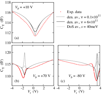
Figure 6: Comparison of theoretical results including disorder for the measured capacitance $C_{Y}$ with experimental data by Young et al.young-arXiv We have taken $\gamma_{1}=0.35\mathrm{eV}$, and $v_{F}=1.05\times 10^{6}\mathrm{ms}^{-1}$.

Figure 6 shows the comparison of data from both disorder models to the experimentsyoung-arXiv of Young et al. In this case, the back gate is kept at a fixed potential while the top gate is varied. This has the effect of simultaneously changing the size of the gap and the carrier density so in this case we treat these two quantities seperately and use the full theory of the inter-layer screening described in Section II to compute the size of the effective gap. When the gap is small at low density (i.e. for $V_{b}=10\mathrm{V}$, plot (a)) the both theories of disorder predict qualitatively correct answers. The difference between the experimental and theoretical curves can be reduced by changing the value of the stray capacitance as a fitting parameter. For very low values of disorder, a small spike is present at zero density in the density averaged data. This is due to the very small band gap that is present and the associated $\delta$-function in $\frac{d\mu}{dn}$. Larger values of disorder smear this divergence out into a dip, the shape of which matches the experimental data well. The DoS averaged plots do not show this dip because carrier density is always finite in this model, and the effect of increasing disorder is to increase the minimum value of the carrier density thus decreasing the depth of the dip. When the gap is large at zero density (i.e. for large back gate voltage, $V_{b}=70\mathrm{V}$, plot (b) and $V_{b}=-80\mathrm{V}$, plot(c)) then the DoS averaging procedure predicts qualitatively wrong results for low values of disorder. There are two main features in the low density part of these plots. First, for finite gap, Fig. 3 shows that $\frac{d\mu}{dn}$ tends to zero as density decreases. This gives a peak in the measured capacitance (because $C_{Y}\propto 1/(\frac{d\mu}{dn}+\frac{e^{2}d_{t}}{\epsilon_{0}\epsilon_{t}})$) which is blurred by finite disorder. The second feature is the $\delta$-function at the band edge (or, equivalently, at zero density) which is broadened by finite disorder in the density averaging model, but which plays no role in the DoS averaging model because this model always gives rise to a finite density of carriers. This means that the DoS average cannot predict correct results in the low-density, finite gap regime. However, the density averaging model does include the effects of the $\delta$-function spike by sampling many values of density, and crucially including $n=0$. This spike in $\frac{d\mu}{dn}$ manifests as the dip in the measured capacitance and parameters can be chosen so that the size and shape of the dip match the experimental data quite closely. We therefore believe the density-averaging procedure of Eq. (7) to be the preferable model for including disorder over the the DoS-averaging model.

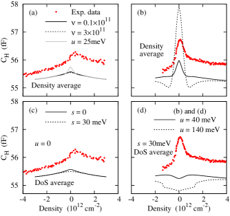
Figure 7: Comparison of theoretical results including disorder with experimental data by Henriksen et al.henriksen-prb82 (a) $u_{\mathrm{ext}}=0$ compared with the density averaged model for zero gap and a small gap; and $u=25\mathrm{meV}$ for $\nu=3\times 10^{11}\mathrm{cm}^{-2}$. (b) $u_{\mathrm{ext}}$ finite, compared with the density averaged theory for several values of the gap. We have taken $\nu=3\times 10^{11}\mathrm{cm}^{-2}$ and the legend is as shown in (d). (c) DoS averaged theory compared with $u_{\mathrm{ext}}=0$ expermimental data for $s=0$ and $s=30\mathrm{meV}$. (d) $u_{\mathrm{ext}}$ finite compared with DoS averaged theory for two values of the gap. $s=30\mathrm{meV}$ in each case. We have taken $\gamma_{1}=0.35\mathrm{eV}$, and $v_{F}=1.05\times 10^{6}\mathrm{ms}^{-1}$ throughout.

This general picture is also seen in the comparison of the two disorder theories with data by Henriksen et al. as shown in Fig. 7. Panels (c) and (d) show the comparison of the experimental data to the DoS averaged model. In this experiment, the measured capacitance is proportional to $\frac{d\mu}{dn}$, so in the gapped case in panel (d), the step in $\frac{d\mu}{dn}$ due to the change in topology of the Fermi surface is clearly seen for large gap. The zero gap data in panel (c) shows qualitatively the correct features, although the stray capacitance must be altered to get a better fit and the peak is taller in the experimental data than in the theory. But when the gap is opened as shown in part (d), the DoS averaged theory predicts qualitatively wrong results because it does not account for the broadened $\delta$-function associated with the band edges. The experimental data also shows a distinct asymmetry between the electron and hole density regimes. This is not explained in our model, but can be added by allowing for an asymmetry in the underlying band structure, for example by including specific next-nearest neighbor hops in the tight binding model.li-prl102 On the other hand, the density-averaging theory (shown in panels (a) and (b)) do predict the correct behavior. For the zero-gap experiment, the variation of the predicted $C_{H}$ is too small, and better agreement can be found by allowing for a small gap to open as shown by the dashed line. In panel (b), it is clear that a gap size of $\approx 40\mathrm{meV}$ gives a semi-quantitative fit to the experiment.

VI Conclusion and discussion

In conclusion, we have presented a full calculation of $\frac{d\mu}{dn}$ (and hence the quantum capacitance and compressibility) for graphene and have discussed two different methods for including disorder effects. These models require averaging the effect of the disorder potential in either the density of states or directly as a variation in the local electron density. We find that when there is no gap in the system, these two models predict qualitatively similar results. But when there is a gap present, the DoS averaging method fails to account for the step in the chemical potential due to the band edges and therefore predicts qualitatively incorrect results. So, we present two conclusions: First, that the single-particle theory for the compressibility of graphenes appears to allow qualitatively good predictions for thermodynamic quantities such as the compressibility. Second, the inclusion of disorder via statistical averaging must be done carefully because the choice of where the averaging is done critically affects the outcome. We find that the averaging should be carried out at the level of the experimental quantity rather than the density of states.

We believe that the effects left out of the theory, particularly the many-body exchange-correlation corrections are likely to be qualitatively unimportant for understanding the experimental data for currently available graphene samples which are dominated by disorder. In particular, disorder effects are strongest at the lowest carrier densities where exchange-correlation effects become more important quantitatively. This makes an observation of many-body effects through compressibility measurements quite challenging.

We thank J. P. Eisenstein, E. A. Henriksen, P. Kim, and A. Young for discussions of their experimental results. This work was supported by US-ONR and NRI-SWAN.

*

Appendix A Analytical results for $K^{h}$

In this Appendix, we give the derivation of $K^{h}$, and write down the full expression for it in various cases. The full form of the indefinite integral in Eq. (5) is

$$I(k) =\frac{2\mathcal{A}}{\pi}\int kE_{k}^{h}\,dk$$

$$=\frac{\mathcal{A}\gamma_{1}^{3}}{\pi\hbar^{2}v_{F}^{2}}\frac{1}{24\sqrt{\Delta}}\bigg{\{}\sqrt{2\Delta}\left(8x-\Phi+1-4\delta^{2}\right)\Xi+$$

$$\qquad\qquad+12\delta^{2}\log\left[2\Delta\left(-\Delta+\Phi+\sqrt{2\Delta}\Xi\right)\right]\bigg{\}}$$

where $x=(\hbar v_{F}k/\gamma_{1})^{2}$, $\delta=u/(2\gamma_{1})$, $\Phi=\sqrt{1+4x\Delta}$, $\Xi=\sqrt{2x-\Phi+1+2\delta}$, and $\Delta=1+4\delta^{2}$. Explicitly differentiating with respect to $k$ verifies the Fundamental Theorem of Calculus which we utilized in the description of Eq. (6). In the general case, the derivative of the energy with respect to the wave vector is

$$\frac{dE_{k_{F}}^{h}}{dk_{F}}=\frac{\hbar^{2}v_{F}^{2}k_{F}}{E_{k_{F}}^{h}}\left(1-\frac{\gamma_{1}^{2}+u^{2}}{2\sqrt{\frac{\gamma_{1}^{4}}{4}+\hbar^{2}v_{F}^{2}k_{F}^{2}(\gamma_{1}^{2}+u^{2})}}\right).$$ (10)

The $u=0$ limit

In this case, $k_{F}=\sqrt{\pi n}$ for all densities. Therefore the derivatives of $k_{F}$ with respect to $n$ are elementary, the $k_{F_{-}}$ terms in Eq. (6) trivially do not contribute and we have

$$K^{h}_{u=0}=\frac{\gamma_{1}}{n_{0}\sqrt{\frac{1}{2}+\frac{n}{n_{0}}-\sqrt{\frac{1}{4}+\frac{n}{n_{0}}}}}\left(\frac{1}{2}-\frac{1}{4\sqrt{\frac{1}{4}+\frac{n}{n_{0}}}}\right)$$

where $n_{0}=\gamma_{1}^{2}/(\pi\hbar^{2}v_{F}^{2})$.

When $u>0$, $|E_{F}|>u/2$

When $|E_{F}|>u/2$ then $k_{F_{+}}=\sqrt{\pi n}$ and $k_{F_{-}}=0$ so that the derivatives with respect to $n$ are elementary and only the first two terms of Eq. (6) contribute to $K^{h}$. Therefore

$$K^{h}(|E_{F}|>\frac{u}{2})=\frac{\gamma_{1}}{2n_{0}\sqrt{\frac{1}{2}+\frac{n}{n_{0}}+\frac{u^{2}}{4\gamma_{1}^{2}}-\sqrt{\frac{1}{4}+\frac{n}{n_{0}}\frac{n_{0u}}{n_{0}}}}}\\ \times\left(1-\frac{n_{0u}/{n_{0}}}{2\sqrt{\frac{1}{4}+\frac{n}{n_{0}}\frac{n_{0u}}{n_{0}}}}\right)$$

where $n_{0u}=(\gamma_{1}^{2}+u^{2})/(\pi\hbar^{2}v_{F}^{2})$.

When $u>0$, $|E_{F}|<u/2$

However, when $|E_{F}|<u/2$ we need to use the expressions for the two Fermi surfaces in Eq. (2) so that

$$\frac{dk_{F_{\pm}}}{dn}=\frac{\pi}{4k_{F_{\pm}}}\left(\frac{n}{n_{0u}}\pm 1\right)$$

and hence

$$\frac{d^{2}k_{F_{\pm}}}{dn^{2}}=\frac{\pi}{4k_{F_{\pm}}}\left[\frac{1}{n_{0u}}-\frac{\pi}{4k^{2}_{F_{\pm}}}\left(\frac{n}{n_{0u}}\pm 1\right)^{2}\right].$$

Substituting these expressions for the derivatives into Eq. (6) gives the simplified expression

$$K^{h}(|E_{F}|<u/2)=\frac{\pi}{8}\bigg{[}\frac{1}{k_{F_{+}}}\left(\frac{n}{n_{0u}}+1\right)^{2}\frac{dE_{k_{F_{+}}}}{dk_{F_{+}}}\\ -\frac{1}{k_{F_{-}}}\left(\frac{n}{n_{0u}}-1\right)^{2}\frac{dE_{k_{F_{-}}}}{dk_{F_{-}}}\bigg{]}$$

where the derivatives of the Fermi energy with respect to the Fermi wave vector are given by making the appropriate substitutions in Eq. (10).

References

- (1) D. S. L. Abergel, V. Apalkov, J. Berashevich, K. Ziegler, and T. Chakraborty, Adv. Phys. 59, 261 (2010).
- (2) S. Das Sarma, S. Adam, E. H. Hwang, and E. Rossi, Rev. Mod. Phys., in press.
- (3) D. L. John, L. C. Castro, and D. L. Pulfrey, J. Appl. Phys. 96, 5180 (2004).
- (4) T. Fang, A. Konar, H. Xing, and D. Jena, Appl. Phys. Lett. 91, 092109 (2007).
- (5) J. Martin, N. Akerman, G. Ulbricht, T. Lohmann, J. H. Smet, K. von Klitzing, and A. Yacoby, Nat. Phys. 4, 144 (2008).
- (6) E. H. Hwang, B. Y.-K. Hu, and S. Das Sarma, Phys. Rev. Lett. 99 226801 (2007).
- (7) A. F. Young, C. R. Dean, I. Meric, S. Sorgenfrei, H. Ren, K. Watanabe, T. Taniguchi, J. Hone, K. L Shepard, and P. Kim, arXiv:1004.5556v2, unpublished.
- (8) E. A. Henriksen and J. P. Eisenstein, Phys. Rev. B 82, 041412(R) (2010).
- (9) J. Xia, F. Chen, J. Li, and N. Tao, Nat. Nano. 4, 505 (2009). See supplementary information for experimental data relating to bilayer graphene.
- (10) S. V. Kusminskiy, J. Nilsson, D. K. Campbell, and A. H. Castro Neto, Phys. Rev. Lett. 100 106805 (2008).
- (11) G. Borghi, M. Polini, R. Asgari, A. H. MacDonald, Phys. Rev. B 82, 155403 (2010).
- (12) R. Sensarma, E. H. Hwang, and S. Das Sarma, e-print arXiv:1102.1427 (unpublished).
- (13) E. McCann and V. I. Fal’ko, Phys. Rev. Lett 96, 086805 (2006).
- (14) E. McCann, Phys. Rev. B 74, 161403(R) (2006).
- (15) T. Stauber, N. M. R. Peres, F. Guinea, and A. H. Castro Neto, Phys. Rev. B 75, 115425 (2007).
- (16) H. Min, B. Sahu, S. K. Banerjee, and A. H. MacDonald, Phys. Rev. B 75, 155115 (2007)
- (17) E. V. Castro, K. S. Novoselov, S. V. Morozov, N. M. R. Peres, J. M. B. Lopes dos Santos, J. Nilsson, F. Guinea, and A. H. Castro Neto, Phys. Rev. Lett. 99, 216802 (2007).
- (18) We find for the experiments of Young, et al. that , , , , , and . For the data of Henriksen et al. we have , , , , and .
- (19) E. Rossi and S. Das Sarma, Phys. Rev. Lett. 101, 166803 (2008); S. Das Sarma, E. H. Hwang, and E. Rossi, Phys. Rev. B 81, 161407 (2010).
- (20) E. H. Hwang and S. Das Sarma, Phys. Rev. B 82, 081409 (2010).
- (21) Z. Q. Li, E. A. Henriksen, Z. Jiang, Z. Hao, M. C. Martin, P. Kim, H. L. Stormer, and D. N. Basov, Phys. Rev. Lett. 102, 037403 (2009); A. B. Kuzmenko, I. Crassee, D. van der Marel, P. Blake and K. S. Novoselov, Phys. Rev. B 80, 165406 (2009).