Transitions to three-dimensional flows in a cylinder driven by oscillations of the sidewall

Abstract

The transition from two-dimensional to three-dimensional flows in a finite circular cylinder driven by an axially oscillating sidewall is explored in detail. The complete symmetry group of this flow, including a spatio-temporal symmetry related to the oscillating sidewall, is $Z_{2}\times O(2)$. Previous studies in flows with the same symmetries, such as symmetric bluff-body wakes and periodically forced rectangular cavities, were unable to obtain the theoretically predicted bifurcation to modulated traveling waves. In the simpler cylindrical geometry, where the azimuthal direction is physically periodic, we have found these predicted modulated traveling waves as stable fully saturated nonlinear solutions for the first time. A careful analysis of the base states and their linear stability identifies different parameter regimes where three-dimensional states that are either synchronous with the forcing or quasiperiodic, corresponding to different symmetry-breaking processes. These results are in good agreement with theoretical predictions and previous results in similar flows. These different regimes are separated by three codimension-two bifurcation points that are yet to be fully analyzed theoretically. Finally, the saturated nonlinear states and their properties in different parameter regimes are analyzed.

1 Introduction

When a system is invariant under the action of a group of symmetries, there can be far-reaching consequences on its bifurcations. When the symmetries are purely spatial in nature (e.g. reflections, translations, rotations), these consequences have been extensively studied (e.g., see Golubitsky & Schaeffer, 1985; Golubitsky, Stewart & Schaeffer, 1988; Crawford & Knobloch, 1991; Cross & Hohenberg, 1993; Chossat & Iooss, 1994; Iooss & Adelmeyer, 1998; Chossat & Lauterbach, 2000; Golubitsky & Stewart, 2002). The system may also be invariant to the action of spatio-temporal symmetries. These are spatial symmetries composed with temporal evolution. A classic example is the two-dimensional Kármán vortex street form of the wake of a circular cylinder. Other common cases are periodically forced flows.

The transition from two-dimensional to three-dimensional flow is of fundamental interest in fluid dynamics. Two-dimensional flows, like the Kármán vortex street and other bluff-body wakes, are invariant in the spanwise direction to both translations ($SO(2)$ symmetry group) and reflections ($Z_{2}$ symmetry group), the combination generating the $O(2)$ symmetry group. We are interested in the transition from two-dimensional to three-dimensional flow when the two-dimensional problem has a spatio-temporal symmetry of $Z_{2}$ type, as is the case for the wake of a circular cylinder in the streamwise direction (Blackburn & Lopez, 2003a; Blackburn, Marques & Lopez, 2005). Another flow with the same spatio-temporal symmetries as the periodically shedding wake is that in a periodically-driven rectangular cavity of infinite spanwise extent (Marques, Lopez & Blackburn, 2004), which has been studied in Lopez & Hirsa (2001); Vogel, Hirsa & Lopez (2003); Blackburn & Lopez (2003b).

The complete symmetry group of these flows is $Z_{2}\times O(2)$. The implications of $O(2)$ symmetry in fluid systems have been studied extensively, both when the instability breaking $O(2)$ symmetry (i.e. transition from two-dimensional to three-dimensional) is due to a single real eigenvalue becoming positive (steady bifurcation) as well as when it is due to a pair of complex-conjugate eigenvalues gaining positive real part, leading to time-periodic flow (e.g. see the references cited above). The types of symmetry-breaking bifurcations to three-dimensional flow that a two-dimensional flow with a space-time symmetry can experience are completely determined by the symmetry group of the system, and not by the particulars of the physical mechanisms responsible for the bifurcation, and have been analyzed in detail in Marques et al. (2004). The main results obtained are that there are two type of bifurcations, one synchronous with the forcing and the other resulting in quasiperiodic flows. Both types come in two different flavors, depending on the symmetries of the bifurcated solutions. There are two synchronous modes, A and B, that break or preserve the space-time symmetry $Z_{2}$, respectively. The quasiperiodic solutions have the form of modulated traveling waves or modulated standing waves in the spanwise direction; they differ in their symmetry properties: the traveling waves preserve a space-time symmetry, while the standing wave preserves a purely spatial reflection symmetry.

In the examples of flows with $Z_{2}\times O(2)$ symmetry group described above, the $O(2)$ invariance is only an idealization of the corresponding experimental flow due to the finite extent of the spanwise direction. The typical result is that the travelling waves predicted by the theory do not travel, due to endwall effects (Leung et al., 2005). Cylindrical geometries are very useful in the sense that the azimuthal direction is physically periodic and have the $O(2)$ symmetry group exactly fulfilled. This fact has been explored in Blackburn & Lopez (2010) in a driven annular geometry, but unfortunately, the modulated traveling wave modes that are predicted from the Floquet analysis do not saturate nonlinearly to pure modes but are always mixed with contributions from the synchronous A mode. In the present paper we explore a simpler setting, a finite circular cylinder with an axially oscillating sidewall. The base state is also $Z_{2}\times O(2)$ invariant as in the other flow examples, and we have indeed found nonlinearly saturated pure modulated travelling waves for the first time in a physically-realizable flow. In this cylindrical setting, as the travelling waves move in the azimuthal direction, i.e. the pattern rotates around the cylinder axis, they will be termed rotating (or modulated rotating) waves.

The paper is organized as follows: in §2 the formulation of the problem and numerical methods used are presented; in §3 the base state of the system is computed, and its changes when parameters are varied are discussed; in §4 the linear stability of the basic flow is studied, and compared with similar flows. In §5 the three-dimensional structure and symmetries of the different unstable modes found are analyzed in detail. Finally, in §6 the main results are summarized and open problems and future directions of study are discussed.

2 Governing equations and numerical methods

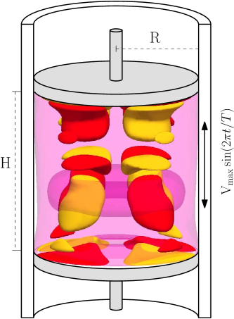
Figure 1: (Color online) Schematic of the apparatus. The inset shows a synchronous bifurcated state; translucent isosurfaces (of azimuthal vorticity) show the axisymmetric roller generated by the side wall oscillation, and solid isosurfaces (of radial vorticity) show the braid structures associated with three-dimensional instabilities.

Consider a Newtonian fluid of kinematic viscosity $\nu$ confined in a finite cylinder of radius $R$ and height $H$, whose sidewall oscillates harmonically in the axial direction, with period $T$ and maximum axial velocity $V_{\max}$, while the top and bottom lids remain at rest, as shown schematically in figure 1. The system is non-dimensionalized taking $R$ as the length scale, and the viscous time $R^{2}/\nu$ as the time scale. There are three non-dimensional parameters in this problem:

Aspect ratio $$\varGamma=H/R,$$ (1)

Reynolds number $$Re=V_{\max}R/\nu,$$ (2)

Stokes number $$St=R^{2}/\nu T.$$ (3)

The aspect ratio defines the geometry of the problem, while $Re$ and $St$ are non-dimensional measures of the amplitude and frequency of the forcing; the inverse of the Stokes number is precisely the non-dimensional period of the oscillations, $\tau=1/St$. In the current study, the aspect ratio is fixed at $\varGamma=2$. The non-dimensional Navier–Stokes equations governing the flow are

$$\Big{(}\frac{\partial}{\partial t}+\mathbf{u}\cdot\nabla\Big{)}\mathbf{u}=-\nabla p+\nabla^{2}\mathbf{u},$$ (4a)

$$\nabla\cdot\mathbf{u}=0,$$ (4b)

where $\mathbf{u}=(u,v,w)$ is the velocity field in cylindrical coordinates $(r,\theta,z)\in[0,1]\times[0,2\pi]\times[-\varGamma/2,\varGamma/2]$, and $p$ is the kinematic pressure, all non-dimensional. The vorticity associated to the velocity field is $\nabla\times\mathbf{u}=(\xi,\eta,\zeta)$. No-slip velocity boundary conditions are used on all walls. The velocity is zero on stationary top and bottom endwalls, and the $z$-component of velocity at the sidewall oscillates periodically in time:

$$\mathbf{u}(r,\theta,\pm\varGamma/2,t)=(0,0,0),$$ (5a)

$$\mathbf{u}(1,\theta,z,t)=\big{(}0,0,Re\sin(2\pi St\,t)\big{)}.$$ (5b)

These idealized boundary conditions are discontinuous at the junctions where the stationary lids meet the oscillating sidewall. In a physical experiment there are small but finite gaps at these junctions where the axial velocity adjusts rapidly to zero. For a proper use of spectral techniques, a regularization of this discontinuity is implemented of the form

$$w(1,\theta,z,t)=Re\sin(2\pi St\,t)\left[1-\exp{\left(-\frac{1-z}{\epsilon}\right)}\right]\left[1-\exp{\left(-\frac{1+z}{\epsilon}\right)}\right]$$ (6)

where $\epsilon$ is a small parameter that mimics the small physical gaps ($\epsilon=6\times 10^{-3}$ has been used as a fixed parameter). The use of $\epsilon\neq 0$ regularizes the otherwise discontinuous boundary conditions; see Lopez & Shen (1998) for further details on the use of this technique in spectral codes.

Instead of having a oscillatory sidewall, we could also consider the situation where the sidewall is at rest, and the two endwalls oscillate harmonically, which in some cases can be more convenient from the experimental point of view. In order to have a fixed domain, it is very useful to write the governing equations in the oscillating reference frame, in which the cylindrical domain is at rest and the sidewall oscillates. However, the oscillating reference frame is not an inertial frame, and inertial body force terms must be included in the Navier–Stokes equations. In this case, there is one extra term, $-{\bf A}/\rho$, where ${\bf A}$ is the acceleration of the lids and $\rho$ is the fluid density. Since the acceleration ${\bf A}$ depends only on time, and for an incompressible flow $\rho$ is constant, this extra term is a gradient that can be incorporated in the pressure term, thereby recovering exactly the same formulation as in the case of oscillatory sidewalls. The difference between oscillating the sidewall or the endwalls is only important when density variations appear, for example in the presence of temperature differences, or concentration differences if the fluid is a mixture.

The governing equations and boundary conditions are invariant to the following spatial symmetries:

$$K_{\theta}(u,v,w)(r,\theta,z,t)=(u,-v,w)(r,-\theta,z,t),$$ (7a)

$$R_{\alpha}(u,v,w)(r,\theta,z,t)=(u,v,w)(r,\theta+\alpha,z,t),$$ (7b)

for any real $\alpha$. $K_{\theta}$ represents reflections about any meridional plane, whilst $R_{\alpha}$ signifies rotations about the cylinder axis. $K_{\theta}$ and $R_{\alpha}$ generate the groups $Z_{2}$ and $SO(2)$, but the two operators do not commute, so the symmetry group generated by $K_{\theta}$ and $R_{\alpha}$ is $O(2)$ and it acts in the periodic azimuthal $\theta$-direction. The horizontal reflection on the mid-plane $z=0$ acts on the velocity field as:

$$K_{z}(u,v,w)(r,\theta,z,t)=(u,v,-w)(r,\theta,-z,t).$$ (8)

However, $K_{z}$ is not a symmetry of the system: due to the harmonic oscillation of the sidewall, the boundary condition (5b) is not $K_{z}$ invariant. However, $K_{z}w(1,\theta,z,t)$ coincides with $w(1,\theta,z,t+T/2)$, introducing an additional spatio-temporal symmetry. Therefore, the system is also invariant to a reflection about the half-height plane $z=0$ together with a half-period evolution in time:

$$H(u,v,w)(r,\theta,z,t)=(u,v,-w)(r,\theta,-z,t+\tau/2).$$ (9)

The transformation $H$ generates another $Z_{2}$ symmetry group that commutes with $O(2)$. Hence, the complete symmetry group of the problem is $Z_{2}\times O(2)$. The action of the spatio-temporal symmetry $H$ on the vorticity is different to the action on the velocity, and is given by:

$$H\left(\xi,\eta,\zeta\right)(r,\theta,z,t)=\left(-\xi,-\eta,\zeta\right)(r,\theta,-z,t+\tau/2).$$ (10)

Therefore, the individual symmetries (and the generated groups) are exactly the same as for the periodically-driven annular cavity and analogous to the two-dimensional time-periodic wake of symmetrical bluff bodies and periodically-driven rectangular cavity flows.

2.1 Numerical formulation

The governing equations have been solved using a second-order time-splitting method. The spatial discretization is via a Galerkin-Fourier expansion in $\theta$ and a Chebyshev collocation in $x=2r$ and $z$, of the form

$$F(r,\theta,z)=\sum_{l=0}^{n_{r}}\sum_{n=0}^{n_{z}}\sum_{m=-n_{\theta}}^{n_{\theta}}a_{l,n,m}T_{l}(x)T_{n}(z)e^{im\theta}$$ (11)

for the three velocity components and pressure. The results presented here were computed with $n_{r}=48$, $n_{z}=96$ and $n_{\theta}=10$. This resolution resolves all the spatial scales in the solutions presented here. Time steps of $\delta t=10^{-5}$ have been required to ensure numerical stability and accuracy of the temporal scheme. For each Fourier mode, the corresponding Helmholtz and Poisson equations are solved efficiently using a complete diagonalization of the operators in both the radial and axial directions. Note that to decouple the Helmholtz equations for $u$ and $v$, we have used the combinations $u_{+}=u+iv$ and $u_{-}=u-iv$. The coordinate singularity at the axis $(r=0)$ is treated following some prescriptions, which guarantee the regularity conditions at the origin needed to solve the Helmholtz equations (see Mercader, Net & Falqués, 1991, for details). The spectral collocation solver used here is based on a previous scheme (Mercader, Batiste & Alonso, 2010) that has recently been tested and used in a wide variety of flows in enclosed cylinders (Marques et al., 2007; Lopez et al., 2007, 2009; Lopez & Marques, 2009).

3 Basic states

	$(a)$ $St=10$	$(b)$ $St=32$	$(c)$ $St=50$	$(d)$ $St=100$
$\psi$
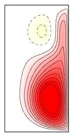
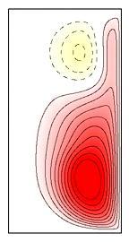
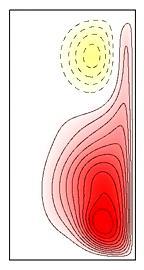
$\eta$

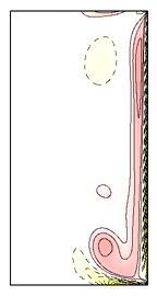
Figure 2: (Color online) Contours of streamfunction, $\psi$, and azimuthal vorticity, $\eta$, of the basic state at four $St$ values as indicated, for amplitudes $Re$ very close to the corresponding critical values. Solid (dashed) contours are positive (negative); light/dark (yellow/red online) colors correspond to negative/positive values. The base state is periodic, and we have selected for each $St$ the phase of period where the oblique jet at the bottom corner is most intense; the associated movies online show temporal evolution over one period.

The basic flow, having the symmetries of the problem, is always axisymmetric and time-periodic, synchronous with the forcing. The axial oscillations of the cylindrical wall produce periodic Stokes-type boundary layers on the oscillating wall. These layers separate from the sidewall and move towards the cylinder axis after colliding with the endwalls to form rollers. These rollers are formed every half period alternatively on each endwall. The term roller refers to large-scale rotating flow structures with primarily azimuthal vorticity, $\eta$. Instantaneous contours of the streamfunction ($\psi$, such that $u=-1/r\,\partial\psi/\partial z$ and $w=1/r\,\partial\psi/\partial r$) are shown in the first row of figure 2 for four increasing values of the forcing frequency $St$, and for amplitudes $Re$ very close to, and above, the critical value at which the basic flow becomes unstable; the online version of the paper includes movies animating these contours over a forcing period. In all cases the figures represent meridional planes $(r,z)\in[0,r]\times[-\varGamma/2,\varGamma/2]$ and the wall is at rest at $t=0$.

The magnitude and size of the rollers changes substantially with $St$. For small forcing frequencies, there is sufficient time for these rollers to dissipate during part of the forcing period, and so in figure 2$(a)$ a single roller fills the whole domain most of the time, whereas for large frequencies the rollers persist at both ends throughout the whole forcing cycle. The Stokes number determines the size of the rollers and their dissipation, and the Reynolds number measures the strength of their collision with the lids and the recirculation of the fluid. The characteristics of the rollers are similar to the ones described in previous works for the planar case (Blackburn & Lopez, 2003b) and for an annular cavity (Blackburn & Lopez, 2010), but in the present analysis the curvature effects are very important, and the flow geometry is substantially altered near the cylinder axis.

Instantaneous contours of the azimuthal vorticity are shown in the second row of figure 2. These contours describe the boundary layers that form at the sidewall and endwalls and their dynamics very well. The sidewall boundary layer is a Stokes-type boundary layer whose thickness is proportional to $St^{-1/2}$ (Schlichting & Kestin, 1979; Marques & Lopez, 1997), so the boundary layer becomes thinner for larger values of the forcing frequency $St$ (it also becomes thinner as the amplitude of the forcing $Re$ is increased). The sidewall boundary layer, dragged by the cylinder sidewall motion, separates upon colliding with the endwalls, and from the corners where the sidewall and endwalls meet, the boundary layer enters the bulk of the fluid, forming axisymmetric oblique jets that result in the formation of the rollers. This process is analogous to the formation of a vortex roller near the junction of an impulsively started plate and a stationary plate, where there is a jump in the velocity (Allen & Lopez, 2007). The jets are clearly seen in the azimuthal vorticity contours: the jet centerline coincides with the azimuthal vorticity zero contour, and on each side it is surrounded by regions with intense azimuthal vorticity of opposite signs. Oscillating boundary layers also form on the endwalls with azimuthal vorticity of opposite sign to that of the rollers, as a result of the jet dynamics just described, and because the endwalls are at rest.

4 Stability of the basic flow

By increasing the amplitude of the forcing $Re$ beyond a critical value $Re_{\textrm{c}}(St)$, the basic state undergoes a symmetry-breaking bifurcation yielding a new three-dimensional state. Depending on $St$, the basic state may undergo either synchronous or Neimark–Sacker bifurcations. The stability of the basic flow has been comprehensively explored for $St\in[1,150]$, revealing two synchronous modes ($A$ and $B$) that bifurcate from the axisymmetric state by breaking the symmetries differently in each case. There is also a novel quasiperiodic mode that manifests as modulated rotating waves MRW. We use subscripts for each of these states to indicate their azimuthal wavenumber $m$.

The linear stability of the basic state to general three-dimensional perturbations has been determined using global linear stability analysis via time evolution of the Navier–Stokes equations (Lopez, Marques, Rubio & Avila, 2009; Do, Lopez & Marques, 2010). First, a periodic axisymmetric basic state was computed at some point in parameter space. Its stability was determined by introducing small random perturbations into all azimuthal Fourier modes. For sufficiently small perturbations, the nonlinear couplings between Fourier modes are negligible (below round-off numerical noise) and the growth rates (real parts of the eigenvalues) and structure of the eigenfunctions corresponding to the fastest growing perturbation at each Fourier mode emerge from time evolution. This is tantamount to a matrix-free generalized power method in which the actions of the Jacobian matrices for the perturbations are given by time integration of the Navier–Stokes equations with the aforementioned initial conditions. This direct numerical technique is very efficient as the exponential growth or decay of the perturbations is established in a relatively short evolution time, and there is no need to evolve the disturbances until they saturate nonlinearly.

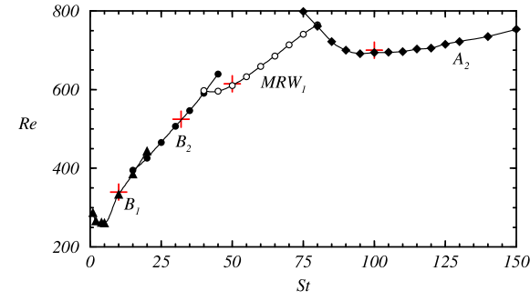
Figure 3: (Color online) Critical Reynolds number, $Re_{\textrm{c}}$, as a function of the Stokes number, $St$, for the transition from the basic state to the different three-dimensional states, $B_{1}$, $B_{2}$, $\mbox{\it MRW}_{1}$ and $A_{2}$. The crosses (red in the online version) correspond to the four basic states depicted in figure 2.

The bifurcation curves for the different modes in $(St,Re)$-space are shown in figure 3. At low $St$, mode $B$ is the first to become critical with increasing $Re$, while at high $St$ mode $A$ is first. At intermediate values $St\in[40.7,79.7]$, the quasiperiodic mode bifurcates first, in the form of modulated rotating waves MRW. The synchronous mode $A$ always has an azimuthal wave number $m=2$ ($A_{2}$), the quasiperiodic mode has $m=1$ ($\mbox{\it MRW}_{1}$), and the synchronous mode $B$ may have either $m=1$ or $m=2$ depending on $St$. The bifurcations to the four different states ($B_{1}$, $B_{2}$, $\mbox{\it MRW}_{1}$ and $A_{2}$) when varying the forcing frequency $St$ are separated by three codimension-two bifurcation points at which two of the states bifurcate simultaneously. The four base states shown in figure 2 correspond to the four distinct bifurcated states in figure 3. The synchronous modes for small $St$ have azimuthal wave number $m=1$ ($B_{1}$) and a single roller fills the domain most of the time, whereas they have azimuthal wave number $m=2$ ($B_{2}$ and $A_{2}$) for larger $St>15$ and two rollers persist throughout the whole forcing cycle. However, the quasiperiodic $MRW_{1}$ has azimuthal wave number $m=1$ although it is dominant in a $St$ region where the two rollers persist.

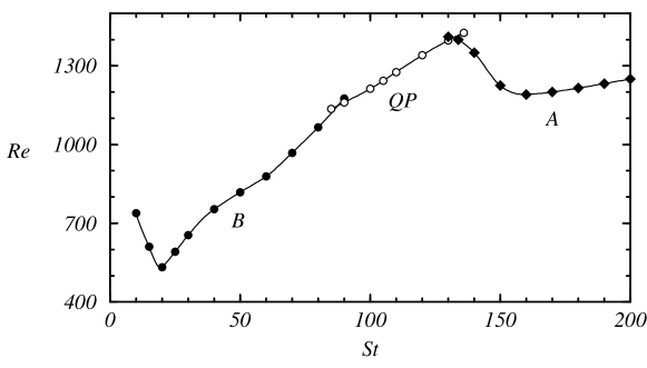
Figure 4: Critical Reynolds number, $Re_{\textrm{c}}$, as a function of the Stokes number, $St$, for the transition from the basic state to the different three-dimensional states, $B$, $QP$ and $A$, for the periodically forced rectangular cavity flow (adapted from Leung et al., 2005).

A very similar scenario occurred in the periodically-driven rectangular cavity problem, as illustrated in figure 4, showing the critical $Re$ number as a function of $St$ in the cavity flow (adapted from Leung et al., 2005). Figures 3 and 4 are strikingly similar, and they only differ in their scaling. The critical $Re$ and $St$ for the rectangular cavity are about a factor of two larger than for the cylinder case, so that the marginal curve in the cavity flow occurs at higher $Re$ number, and the different modes are shifted to higher $St$. The qualitative shape of the marginal curves are very similar in both cases, and the shift in $(St,Re)$ reflects the different geometries of the two problems. An important difference between the two problems is that in the driven rectangular cavity the wavenumber of the bifurcated solution varies continuously, while in the cylinder problem it is discrete (and in fact of very small wavenumber, either $m=1$ or $m=2$). However, the qualitative trend is the same in both problems. In the driven rectangular cavity, the wavenumber of mode $B$ increases with $St$, while for $QP$ and $A$ their wavenumbers are almost independent of $St$ (Leung et al., 2005). In the cylinder problem, the azimuthal wave number of mode $B$ also increases with $St$ (varying from $m=1$ to $m=2$), while for MRW and $A$ their azimuthal wave numbers do not vary with $St$ ($m=1$ for MRW and $m=2$ for $A$).

A detailed comparison with the annular cavity problem (Blackburn & Lopez, 2010) is not possible, because that study focused on the analysis of the modulated rotating waves, that unfortunately where unstable and resulted in complicated flows with mixed characteristics between the synchronous and quasiperiodic solutions. Also, they only considered a single value of $St=100$ at which the traveling wave state was expected to be found. Nevertheless, the different modes obtained here were also present in the annular cavity problem. The radius ratio used in the annular study was close to one, so that both inner and outer radii were much larger than the annular gap. That choice was made to compare with the rectangular cavity flow problem, which corresponds to the radius-ratio-going-to-one limit. As a result, the azimuthal wave numbers of the bifurcating states were very large (between $m=30$ and $m=35$ for the dominant modes in the parameter regime considered). In contrast, in the cylinder problem which corresponds to radius ratio zero (the inner cylinder does not exist so that the outer radius and the gap coincide), the azimuthal wave numbers are very small ($m=1$ and $m=2$). Furthermore, even though the two problems have the same symmetry group, the flow domain in the cylinder is singly-connected whereas in the annulus it is doubly-connected.

5 Three-dimensional structure and symmetries of the unstable modes

After perturbing the axisymmetric basic flow with $Re>Re_{\textrm{c}}(St)$, a new three-dimensional periodic or quasiperiodic state is reached, after waiting enough time for saturation. This bifurcated state depends strongly on the mode that drives the instability, and on the precise values of $(St,Re)$. When describing these bifurcated flows, we will use the term braid, of widespread use in similar flows, to denote smaller-scale meridional structures with vorticity components $\xi$ and $\zeta$. Braids are typically generated through the amplification of spanwise-orthogonal perturbations of the rollers in rectangular cavities, and in cylindrical and annular geometries it is the amplification of meridional perturbations of the rollers that gives rise to the braids.

In the following subsections the symmetries and features of the different bifurcated solutions are described and illustrated with results computed at given values of $St$. Modes $B_{1}$, $B_{2}$ and $A_{2}$ are computed at $St=10$, 32, 100, respectively, whilst mode $\mbox{\it MRW}_{1}$ has been computed at $St=50$, and the corresponding base states have already been illustrated in figure 2. All the solutions have been computed at $Re$ slightly above $Re_{\textrm{c}}$.

5.1 Synchronous modes

Figure 5: $(a)$ Time series of the energies of the leading Fourier modes for the $B_{2}$ state at $Re=525$ and $St=32$; and $(b)$ a close-up of $E_{2}(t)$ after saturation, over two forcing periods.

Three-dimensional states result when a single purely real eigenvalue crosses the unit circle at $+1$ in the complex plane. When an axisymmetric flow that belongs to the synchronous region is perturbed, the energies of the Fourier modes may grow or decay depending on the case, but what is clear is the modulation of the energies with the sidewall frequency. When the basic flow is unstable to synchronous modes, the Fourier spectra begin to grow and at some time reach an asymptotic state where the modes are saturated but oscillate with the driving frequency of the wall around a mean value. Such an evolution can be seen in figure 5, where the energies of the leading Fourier modes are shown as a function of time for the $B_{2}$ state at $Re=525$ and $St=32$; the inset show the oscillations in the energy, synchronous with the forcing (period $\tau=1/St=0.04$), but with the period halved because the energy is a sum of squares of the velocities.

$(a)$ $B_{1}$	$(b)$ $B_{2}$	$(c)$ $A_{2}$

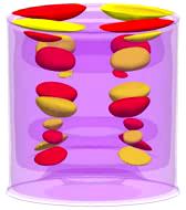
Figure 6: (Color online) Isosurfaces of radial vorticity $\xi$ (solid) and azimuthal vorticity $\eta$ (translucent) for the synchronous states $(a)$ $B_{1}$ at $(Re,St)=(340,10)$ with $\xi=\pm 50$ and $\eta=\pm 500$, $(b)$ $B_{2}$ at $(Re,St)=(525,32)$ with $\xi=\pm 40$ and $\eta=\pm 1000$, and $(c)$ $A_{2}$ at $(Re,St)=(700,100)$ with $\xi=\pm 150$ and $\eta=\pm 800$. The associated movies online show temporal evolution over one forcing period.

The three-dimensional structures of modes $A$ and $B$ are visualized in figure 6 with the aid of perspective views of instantaneous isosurfaces of the radial vorticity (dark/light, or yellow/red in the online movies, are positive/negative values), which shows the braid structures, and azimuthal vorticity (translucent), showing the rollers. Note that the only component of vorticity of the axisymmetric base state that is non-zero is the azimuthal component, and that the braids are comprised of radial and axial components of vorticity and are a direct result of breaking axisymmetry. In general terms, braids are located near the lids and away from the sidewall, and they are born on the oblique jets alternatively emerging from the top and bottom corners. Nevertheless, there are some subtle variations. For $A_{2}$, braids suffer slight changes in shape and their behavior is quite regular as is that of the rollers. Notice that the shape of each roller stays essentially the same as those of the base state. For $B_{1}$ and $B_{2}$, braids change abruptly during a forcing cycle, as do the rollers in this regime, and their dynamics (creation, merging and destruction) are much more complex. In addition, the azimuthal vorticity of the $B$ modes is very different to that of the corresponding basic state.

	$B_{1}$	$B_{2}$	$A_{2}$
$(a)$
$(b)$

Figure 7: (Color online) Axial vorticity contours in a $z$-constant plane of the eigenfunctions at the bifurcation to states $B_{1}$, $B_{2}$ and $A_{2}$ shown in figure 6; $(a)$ is computed at a convenient time $t_{0}$ and $z=\varGamma/4$, while $(b)$ is computed at time $t_{0}+\tau/2$ and $z=-\varGamma/4$, i.e. applying the space-time transformation $H$ to $(a)$. Solid (dashed) contours are positive (negative); light/dark (yellow/red online) colors correspond to negative/positive values.

As the bifurcated solutions are no longer axisymmetric, the $O(2)$ symmetry has been broken, and there only remains the discrete symmetry $R_{2\pi/m}$, a rotation of angle $2\pi/m$ around the axis, where $m$ is the azimuthal wave number of the bifurcated solution. This rotation generates the so-called $C_{m}$ (or $Z_{m}$) symmetry group; when $m=1$ this group is trivial (containing only the identity), and all the rotational symmetries are destroyed. Now, let us examine what happens with the spatio-temporal symmetry $H$. We have plotted in figure 7 axial vorticity contours of the critical eigenvectors for the $B_{1}$, $B_{2}$ and $A_{2}$ bifurcations in a horizontal section $z=\varGamma/4$ for a given time, and in the reflection-symmetric section $z=-\varGamma/4$ after advancing half the forcing period. The figure shows that the bifurcations to $B_{1}$ and $B_{2}$ are $H$-symmetric, i.e. the values of the axial vorticity $\zeta$ of the eigenfunctions, at a given time $t_{0}$ and at $z=\varGamma/2$ (figure 7$a$), are the same as the values of $\zeta$ advancing time by half the forcing period, $t_{0}+\tau/2$, on the reflection-symmetric plane $z=-\varGamma/2$ (figure 7$b$). The eigenfunction of the $A_{2}$ bifurcation is not $H$-symmetric, but changes sign, so the $H$-symmetry is broken in this bifurcation. However, $H$ combined with the rotation $R_{\pi/m}$, with $m=2$ (half the angle of the rotational symmetry of the state), results in a space-time symmetry of the $A_{2}$ eigenfunction. This is precisely the expected behavior from bifurcation theory (Marques et al., 2004): there are only two options for three-dimensional synchronous eigenfunctions under the action of the space-time symmetry $H$, multiplication by $\pm 1$. The behavior of all the velocity and vorticity components is given by

$$H \left\{\begin{array}[]{l}(u,v,w)(r,\theta,z,t)=(u,v,-w)(r,\theta,-z,t+\tau/2),\\ (\xi,\eta,\zeta)(r,\theta,z,t)=(-\xi,-\eta,\zeta)(r,\theta,-z,t+\tau/2),\end{array}\right.$$ preserved: (14)

$$H \left\{\begin{array}[]{l}(u,v,w)_{\textrm{e}}(r,\theta,z,t)=(-u,-v,w)_{\textrm{e}}(r,\theta,-z,t+\tau/2),\\ (\xi,\eta,\zeta)_{\textrm{e}}(r,\theta,z,t)=(\xi,\eta,-\zeta)_{\textrm{e}}(r,\theta,-z,t+\tau/2),\end{array}\right.$$ broken: (17)

$$R_{\pi/m}H \left\{\begin{array}[]{l}(u,v,w)(r,\theta,z,t)=(u,v,-w)(r,\theta+\pi/m,-z,t+\tau/2),\\ (\xi,\eta,\zeta)(r,\theta,z,t)=(-\xi,-\eta,\zeta)(r,\theta+\pi/m,-z,t+\tau/2),\end{array}\right.$$ preserved: (20)

	$B_{1}$	$B_{2}$	$A_{2}$
$(a)$
$(b)$

Figure 8: (Color online) Axial vorticity contours in a $z$-constant plane of nonlinear saturated states corresponding to $B_{1}$, $B_{2}$ and $A_{2}$ shown in figure 6; $(a)$ is computed at a convenient time $t_{0}$ and $z=\varGamma/4$, while $(b)$ is computed at time $t_{0}+\tau/2$ and $z=-\varGamma/4$, i.e. applying the space-time transformation $H$ to $(a)$. Solid (dashed) contours are positive (negative); light/dark (yellow/red online) colors correspond to negative/positive values.

The space-time symmetries of the eigenfunctions translates to the nonlinear saturated states (as long as no additional bifurcations take place in the saturation process). However, the multiplication by -1 shown in (17) is a property of the eigenfunction that the saturated states do not have. The reason is that the eigenfunctions are pure Fourier modes in the azimuthal direction, and when they develop to fully nonlinear three-dimensional bifurcated solutions, Fourier harmonics appear, and the even harmonics (including the zero mode) are multiplied by $(-1)^{2}=+1$ under the action of the $H$-symmetry, so the full nonlinear solution does not have the multiplication by -1 property that the eigenfunction has. Figure 8 shows the same information as in figure 7, but for the full nonlinear bifurcated solutions, illustrating the symmetry properties of the saturated states. The behavior labeled by the subscript e in (17), corresponding to multiplication by -1 under the action of the $H$-symmetry, is no longer present in the saturated nonlinear solution. However, the preserved symmetries $H$ (14) and $R_{\pi/m}H$ (20) clearly persist.

$(a)$ B1	$(b)$ B2	$(c)$ A2

Figure 9: Time average of the energy of the dominant mode for the synchronous solutions as a function of $Re$, $(a)$ B1 solutions at $St=10$, $(b)$ B2 solutions at $St=$, and $(c)$ A2 solutions at $St=100$. The diamond corresponds to the critical $Re$ obtained by linear stability analysis and the solid disks correspond to computed nonlinear solutions.

The three bifurcations to $B_{1}$, $B_{2}$ and $A_{2}$ are supercritical, as shown in figure 9, where the time-averaged energy of the dominant mode $\langle E_{m}\rangle$ is plotted as a function of the Reynolds number; there is no hysteresis, and the behavior of $\langle E_{m}\rangle$ is linear as $Re$ approaches the critical value ($\blacklozenge$). The normal form for the amplitude of the bifurcated synchronous solutions in the supercritical case is given by $\dot{A}=A(\mu-c|A|^{2})$. When saturation is reached, $\dot{A}=0$ and we have $Re-Re_{\textrm{c}}=\mu=c|A|^{2}=d\langle E_{m}\rangle$, the observed linear behavior close to the bifurcation point.

5.2 Quasiperiodic mode

The onset of the quasiperiodic states occurs when two complex-conjugate pairs of eigenvalues cross the unit circle, thus introducing a second frequency $\omega_{Q}$ related to the phase of the complex-conjugate pairs. Generically this second frequency will be incommensurate with the forcing frequency, so the $H$-symmetry is broken in this bifurcation. The second frequency $\omega_{Q}$ can manifest itself in two ways, depending on whether the bifurcation breaks $K_{\theta}$ or $R_{\alpha}$ of the $O(2)$ symmetry of the basic state. In the linear stability analysis we referred only to mode $\mbox{\it MRW}_{1}$, but this term encompasses modulated $\theta$-travelling wave (MRW) and modulated standing wave (MSW) states. Due to the $O(2)$ symmetry of the governing equations, there are two pairs of complex conjugate eigenvalues that bifurcate simultaneously, and they correspond to modulated $\theta$-travelling waves, that can travel in the positive or negative $\theta$-direction; after a period of the forcing, the flow pattern repeats itself, but rotated a certain angle, $\pm\theta_{0}$, related to the second frequency by $\theta_{0}=2\pi\omega_{Q}/St$, where $St=\omega_{f}$ is the forcing frequency. $K_{\theta}$ transforms each one of the MRW into the other, therefore the $K_{\theta}$-symmetry is broken; the $SO(2)$ rotational symmetry is also broken, because the solution has azimuthal wave number $m=1$ ; however, as they are modulated traveling waves, there is a preserved space-time symmetry, consisting in advancing one forcing period in time combined with the rotation $R_{\pm\theta_{0}}$.

Besides the two MRW solutions, there is also a third nonlinear solution corresponding to a symmetric combination of the two MRW states; these states, called modulated standing waves MSW, are $K_{\theta}$-symmetric, but the $SO(2)$ rotational symmetry is completely broken. Only one of the two families of solutions, MRWand MSW, is stable (Marques et al., 2004). In the present problem, as in the case for the driven annular cavity (Blackburn & Lopez, 2003b) and for the driven annular cavity (Leung et al., 2005), the stable solutions are MRW; their sense of travel depends on the initial condition for the sign of the azimuthal velocity perturbation. In order to obtain MSW, it is necessary to enforce the $K_{\theta}$ symmetry, restricting the computations to the appropriate Fourier subspace.

When an axisymmetric flow unstable to $\mbox{\it MRW}_{1}$ mode is perturbed, the energies of all Fourier modes begin to grow with the driving frequency and this is additionally modulated by the quasiperiodic frequency, which is approximately one order of magnitude smaller than the forcing frequency, and it is the same for MRW and MSW states. However, when MSW reaches a saturated state, the energy of the Fourier modes retain both characteristic times, whilst the quasiperiodic frequency for MRW, being related to the azimuthal precession of the pattern, does not manifest in the energy of the Fourier modes.

$(a)$ $\mbox{\it MRW}_{1}$	$(b)$ $\mbox{\it MSW}_{1}$

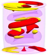
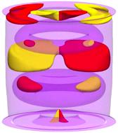
Figure 10: (Color online) Isosurfaces of radial vorticity $\xi$ (solid) and azimuthal vorticity $\eta$ (translucent) for $(a)$ $\mbox{\it MRW}_{1}$ with $\xi=\pm 180$, and $(b)$ $\mbox{\it MSW}_{1}$ with $\xi=\pm 120$, both with $\eta=\pm 1000$ and computed at $(Re,St)=(615,50)$; only $\mbox{\it MRW}_{1}$ is stable. Light/dark (yellow/red online) solid colors correspond to negative/positive values of $\xi$. The associated movies online show temporal evolution over several forcing periods.

The three-dimensional structures of these quasiperiodic flows are visualized in figure 10 by means of perspective views of instantaneous isosurfaces of the axial vorticity (dark/light are positive/negative values) and azimuthal vorticity (translucent). Braids are concentrated on the cylinder endwalls away from the sidewall and suffer large variations in all cases. As with the synchronous modes, the braids seem to be born along the oblique jets emerging from the corners and propagate into the interior, interacting in a complex way with the braids coming from the other endwall. Nevertheless, for MSW the braids possess very regular shapes and look quite similar to those of the synchronous states, and the rollers are virtually not distorted. For MRW however, the braids have a helical structure and the rollers do not resemble the corresponding base flow rollers at all. In fact, the rollers in MRW are tilted with respect to the horizontal rollers in the base state.

	$t=0$	$t=10T$	$t=20T$	$t=30T$
$\mbox{\it MRW}_{1}$
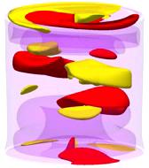
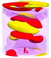
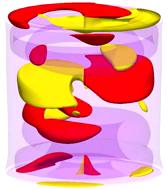
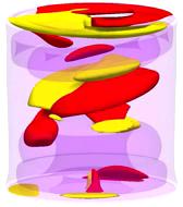
$\mbox{\it MSW}_{1}$

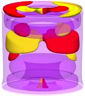
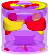
Figure 11: (Color online) Same solutions and isosurface levels as in figure 10, but strobed every 10 forcing periods. The associated movies online show temporal evolution strobed every forcing period.

Figure 11 shows the same contours as in figure 10, all at the same phase at integer multiples of the forcing period apart. For MRW, the strobed structures do not change in a frame of reference that rotates in the azimuthal by an angle $\theta_{0}$ every forcing period, justifying the name of modulated rotating wave. For the MRW shown in figures 10 and 11 at $(Re,St)=(615,50)$, this value is $\theta_{0}\approx 28.77^{\circ}$. This results in a precession frequency $\omega_{p}=3.996$. For MSW, the strobed structures vary substantially in one period, as can be seen in the movie associated with figure 11$(b)$. In general, the ratio between the quasiperiodic and wall periods are not commensurate, and the flow structure never repeats itself. However, the flow structure of MSW remains almost unchanged after ten forcing periods, as shown in figure 11$(b)$; the only noticeable difference is the formation of braids very close to the bottom lid. This is because the ratio of quasiperiodic to forcing frequencies is very close to $1/10$ for the parameter values $(Re,St)=(615,50)$ of MSW; this will be explored in more detail at the end of the present section.

Figure 12: Time average of the energy of the $m=1$ dominant mode for the quasiperiodic solutions as a function of $Re$, for $St=50$. The diamond corresponds to the critical $Re$ obtained by linear stability analysis. Symbols correspond to computed saturated solutions, and the curves are best fits to the parabolic profiles predicted by normal form theory.

The quasiperiodic bifurcation is subcritical, for both MRW and MSW, in contrast to the synchronous bifurcations which are supercritical. Figure 12 shows the time average of the energy of the $m=1$ dominant mode for the quasiperiodic solutions, $\langle E_{1}\rangle$, as a function of the Reynolds number. The MRW solutions show a well-defined hysteretic region; for the MSW, the hysteretic region is very costly computationally to obtain, having extremely long transients. Nevertheless, the energies do not behave linearly close to the critical Reynolds $Re_{\textrm{c}}=610.47$ for $St=50$. We can fit the computed energy amplitudes to the shape predicted by normal form theory. According to Marques et al. (2004), the amplitudes of the bifurcated solutions vary as

$$Re-Re_{\textrm{c}}=\mu=a|A|^{4}-b|A|^{2}=a\langle E_{1}\rangle^{2}-b\langle E_{1}\rangle,$$ (21)

where a quartic term has been included due to the subcritical nature of the bifurcation. The fitting parameters $a$ and $b$ can be expressed in terms of the energy and $Re$ at the saddle-node point:

$$\frac{Re-Re_{\textrm{c}}}{Re_{\textrm{c}}-Re_{\mathit{SN}}}=\frac{\langle E_{1}\rangle}{\langle E_{1}\rangle_{\mathit{SN}}}\biggr{(}\frac{\langle E_{1}\rangle}{\langle E_{1}\rangle_{\mathit{SN}}}-2\biggr{)}.$$ (22)

The solid lines in figure 12 are best fits of this expression to the computed values. The agreement is very good and provides good estimates of the Reynolds numbers of the saddle-node bifurcations. The estimates are $Re_{\mathit{SN}}\approx 610.28$ for MSW and $Re_{\mathit{SN}}\approx 608.57$ for MRW.

$(a)$	$(b)$

Figure 13: $(a)$ Power spectral density of the FFT for MSW at $(Re,St)=(615,50)$ and $(b)$ Poincaré section of the same solution strobing MSW every $\tau$. Symbols $\bullet$ and numbers in $(b)$ corresponds to successive iterates, showing that the frequency ratio is close to rational: $\omega_{Q}/\omega_{f}\approx 1/10$.

The frequencies of the quasiperiodic states can be computed via FFT of the time series of a convenient variable; here we have chosen the value of the axial velocity at a point $P$ close to the sidewall at the cylinder mid-height, $(r,\theta,z)_{P}=(0.9,0,0)$. Figure 13$(a)$ shows the power spectral density for MSW at $(Re,St)=(615,50)$. It is a quasiperiodic spectrum with two well-defined frequencies, $\omega_{f}=50$ and $\omega_{Q}=5.035$, and their linear combinations. The ratio of the frequencies is close to resonance, $\omega_{Q}/\omega_{f}=0.1007\approx 1/10$, and so a small frequency corresponding to $10\omega_{Q}-\omega_{f}\approx 0.353$ is also present. The FFT supplies $\omega_{Q}$ up to a multiple of the forcing frequency; its precise value must be obtained by other methods. In order to analyze in detail how close to resonance the Neimark–Sacker bifurcation is and also to confirm the value of the second frequency, we have computed Poincaré sections of the quasiperiodic states by strobing the MSW solution every period $\tau$. The Poincaré section is shown in Figure 13$(b)$, where we have projected the infinite-dimensional phase space into the plane corresponding to the values of the axial velocity $w$ at two different locations $P$ and $Q$ in the cylindrical domain. The point $P$ is the same used for computing the FFT, at $(r,\theta,z)_{P}=(0.9,0,0)$, and $Q$ is close to the bottom endwall at $(r,\theta,z)_{P}=(0.9,0,-0.1)$. The closed curve is the section of the two-torus where the solution lives, and the symbols $\bullet$ correspond to successive iterates that are numbered in the figure. The tenth iterate, after $10\tau$, almost coincides with the initial point. We have plotted 50 iterates, so we have 10 clusters of 5 points, showing that the rotation number (the ratio of the frequencies $\omega_{Q}/\omega_{f}$) is very close to $1/10$. This justifies the selection of $\omega_{Q}=5.035$ from the FFT.

Figure 14: $(a)$ Power spectral density of the FFT for MRW at $(Re,St)=(615,50)$ and $(b)$ Poincaré section of the same solution strobing MRW every $\tau$. Symbols $\bullet$ and numbers in $(b)$ corresponds to successive iterates, showing that the frequency ratio is close to rational: $\omega_{Q}/\omega_{f}\approx 2/25$.

Figure 14$(a)$ shows the power spectral density for MRW at $(Re,St)=(615,50)$. The second frequency is $\omega_{Q}=3.996$, quite different and smaller than the frequency of MSW. In this case we are even closer to resonance, but a different one. From the Poincaré section in figure 13$(b)$, we see that the iterates undergo two turns on the section before almost coinciding with the initial point after 25 iterates, so now the rotation number (frequency ratio) is $\omega_{Q}/\omega_{f}=0.07992\approx 2/25$, and a very small frequency appears, $2\omega_{f}-25\omega_{Q}\approx 0.1$. Here, we can also estimate $\omega_{Q}$ by measuring the angle $\theta_{0}$ rotated by the flow pattern after one forcing period $\tau$, and the result is in fully agreement with the Poincaré section method.

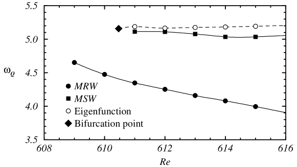
Figure 15: Computed frequencies $\omega_{Q}$ of the quasiperiodic states MRW and MSW as a function of $Re$. Also included are the frequencies of the most unstable eigenfunction, and the critical value $\blacklozenge$.

The frequencies of MRW and MSW for $(Re,St)=(615,50)$ are different, and so we have explored $\omega_{Q}$ as a function of $Re$, for fixed $St=50$; the results are shown in figure 15. We have also plotted the critical frequency at the bifurcation point, $\omega_{Q,\textrm{c}}=5.1572$, and the value of $\omega_{Q}$ for the most dangerous eigenfunction as a function of $Re$. What we observe is that the second frequency for the eigenfunction is almost constant, as is that for MSW with $\omega_{Q}$ slightly smaller than the critical frequency $\omega_{Q,\textrm{c}}$. In contrast, the second frequency of MRW is substantially smaller than the critical value, and it decreases with $Re$, the amplitude of the forcing. This is probably related to the fact that the energy of the MRW is much larger than the energy of MSW, and also to the larger subcriticality of the modulated rotating waves, as shown in figure 12.

We see from figure 15 that the second frequency $\omega_{Q}$, for the MRW and MSW at $(Re,St)=(615,50)$, which are the ones we have discussed in detail in this study, is very close to 4 and 5 respectively. As the forcing frequency is $St=50$, the ratio $\omega_{Q}/\omega_{f}$ is very close to rational (2/25 and 1/10 respectively), as we have already discussed when measuring the frequencies via FFT and Poincaré sections. Of course, along the curves $\omega_{Q}(Re)$, other resonances can be located, but all of them have large denominators, so we do not expect any new dynamics associated with these resonances (Kuznetsov, 2004).

6 Conclusions

Several fluid systems with complete symmetry group $Z_{2}\times SO(2)$ have been explored in recent years. The interest in these flows was triggered by the analysis of symmetric bluff body wakes (see a summary in Blackburn et al., 2005), starting with circular cylinders, and followed by other symmetric bodies, the square cylinder and a flat plate. Flows driven by the periodic motion of one of the container walls resulted in systems with the same symmetry group, and previous studies have analyzed the rectangular driven cavity (Blackburn & Lopez, 2003b; Leung et al., 2005) and a driven annular cavity (Blackburn & Lopez, 2010). As the symmetry group of all these flows is the same, dynamical systems analysis (Marques et al., 2004) predicts the type of bifurcations they can undergo, which are the same in all cases regardless of the specifics of the problem and of the physical mechanisms at work. There are only three possibilities for the transition from the basic state to three-dimensional flows: synchronous modes preserving or breaking the space-time symmetry $H$ or quasiperiodic modes, that come in two flavors, either modulated travelling waves or modulated standing waves. The synchronous modes with the corresponding symmetry properties have been observed in all of these various flow problems. The quasiperiodic modes however have been much more elusive. In symmetric bluff-body wake problems, the quasiperiodic modes do not manifest themselves as primary bifurcations, and can only be observed or computed as secondary or higher bifurcations, in the form of mixed modes. In periodically driven flows, as there are more control parameters, they have been observed in the rectangular driven cavity, but unfortunately spanwise endwalls effects, effectively breaking the $O(2)$ symmetry, resulted in modulated travelling waves that do not travel. In the annular driven geometry with large radius ratios, the quasiperiodic modes are of very high azimuthal wavenumber and have not been found as nonlinearly saturated pure modes, but instead they are mixed complicated modes.

In the present study, we have analyzed the simplest geometry available with the correct symmetries, the cylindrical driven cavity with moderate aspect ratio. This geometry has two advantages over previous studies. First, the $O(2)$ symmetry is exactly fulfilled by the cylindrical geometry (periodicity in the azimuthal direction), eliminating the spanwise endwall effects of the rectangular cavity. And second, the bifurcated states have small azimuthal wavenumbers (typically $m=1$ or 2), so the competition between different modes is greatly reduced. As a result, we have been able to compute nonlinearly saturated pure modulated standing and traveling waves for the first time, and we have also found the two types of synchronous modes, in the appropriate parameter ranges.

As a starting point of the analysis, the periodic synchronous base states have been computed for different forcing amplitudes, $Re$, and forcing frequencies, $St$. These are non-trivial states, with axisymmetric rollers forming alternatively close to each of the endwalls due to the periodic oscillation of the cylinder sidewall. This oscillation produces axisymmetric jets of azimuthal vorticity, emerging from the corners, moving into the interior, and forming the rollers.

The linear stability analysis of the base state has resulted in the computation of the marginal stability curve, shown in figure 3. We have found synchronous bifurcations preserving the $H$ symmetry for small forcing frequencies $St$, and breaking $H$ for larger $St$ values. In between, for intermediate $St$ values, we have found a transition to quasiperiodic solutions. The form of the instabilities is always the same, the formation of braids that are small-scale meridional perturbations of the rollers. The size and persistence of these braids depends strongly on $St$. These results are in good agreement with previous results in flows with the same symmetries, in particular with the driven rectangular cavity problem.

We have also computed saturated nonlinear states, and in all cases sufficiently close to the bifurcation curve, these are pure modes that we have analyzed in detail. The quasiperiodic stable solutions in the present problem are modulated rotating waves, and by restricting the computations to the appropriate subspace, we have also been able to compute the corresponding unstable modulated standing waves. As a result of these nonlinear simulations, we have established that the bifurcations to synchronous states are supercritical, while the bifurcations to quasiperiodic states are subcritical. A careful analysis of the quasiperiodic frequency $\omega_{Q}$ of the modulated standing waves has shown that $\omega_{Q}$ is almost constant and close to the frequency that emerges from the linear stability analysis for the modulated standing waves, whereas the modulated rotating waves exhibit a smaller frequency $\omega_{Q}$ that varies significantly with $St$. Finally, we have found in preliminary explorations to higher $Re$ (i.e. increasing the forcing amplitude) that the three-dimensional pure modes undergo secondary bifurcations to complicated mixed modes for moderate increments in $Re$ beyond critical.

Future directions include an examination of the dynamics in the neighborhood of the codimension-two points where two distinct modes bifurcate simultaneously; these codimension-two points act as organizing centers of the dynamics, and are very likely associated with the secondary bifurcations to mixed modes and more complex dynamics. We have found three codimension-two bifurcations, one associated with the competition between modes B1 and B2, and two on each side of the quasiperiodic region. The codimension-two bifurcation between B1 and B2 is a 1:1 resonance preserving $H$-symmetry, that has been fully studied theoretically (Kuznetsov, 2004). The other two bifurcations are more complex, they are bifurcations of maps with a real eigenvalue (either $\pm 1$) and a pair of complex conjugate eigenvalues of modulus 1, where the $H$-symmetry plays a key role. Although there are some partial results on these bifurcations, they have not been yet fully analyzed (Kuznetsov, 2004), and here we have a physically realizable fluid dynamics system in which they occur. Studies in fluids have been instrumental in developments in nonlinear dynamics, allowing for unified understanding of complex dynamics in a wide spectrum of fields. We hope that this driven cylinder system can help further address some general open questions in dynamical systems. Moreover, this is a relatively easy system in which to conduct experimental research, and we hope experiments in this system will be undertaken in the near future.