Identification, Inference and Sensitivity Analysis for Causal Mediation Effects

Abstract

Causal mediation analysis is routinely conducted by applied researchers in a variety of disciplines. The goal of such an analysis is to investigate alternative causal mechanisms by examining the roles of intermediate variables that lie in the causal paths between the treatment and outcome variables. In this paper we first prove that under a particular version of sequential ignorability assumption, the average causal mediation effect (ACME) is nonparametrically identified. We compare our identification assumption with those proposed in the literature. Some practical implications of our identification result are also discussed. In particular, the popular estimator based on the linear structural equation model (LSEM) can be interpreted as an ACME estimator once additional parametric assumptions are made. We show that these assumptions can easily be relaxed within and outside of the LSEM framework and propose simple nonparametric estimation strategies. Second, and perhaps most importantly, we propose a new sensitivity analysis that can be easily implemented by applied researchers within the LSEM framework. Like the existing identifying assumptions, the proposed sequential ignorability assumption may be too strong in many applied settings. Thus, sensitivity analysis is essential in order to examine the robustness of empirical findings to the possible existence of an unmeasured confounder. Finally, we apply the proposed methods to a randomized experiment from political psychology. We also make easy-to-use software available to implement the proposed methods.

, and

1 Introduction

Causal mediation analysis is routinely conducted by applied researchers in a variety of scientific disciplines including epidemiology, political science, psychology and sociology (see MacKinnon, (mack08, 2008)). The goal of such an analysis is to investigate causal mechanisms by examining the role of intermediate variables thought to lie in the causal path between the treatment and outcome variables. Over fifty years ago, Cochran coch57 (1957) pointed to both the possibility and difficulty of using covariance analysis to explore causal mechanisms by stating: “Sometimes these averages have no physical or biological meaning of interest to the investigator, and sometimes they do not have the meaning that is ascribed to them at first glance” (page 267). Recently, a number of statisticians have taken up Cochran’s challenge. Robins and Greenland robigree92 (1992) initiated a formal study of causal mediation analysis, and a number of articles have appeared in more recent years (e.g., Pearl, (pear01, 2001); Robins, 2003; Rubin, 2004; Petersen, Sinisi and van der Laan, 2006; Geneletti, 2007; Joffe, Small and Hsu, 2007; Ten Have et al., 2007; Albert, 2008; Jo, 2008; Joffe et al., 2008; Sobel, 2008; VanderWeele, 2008, 2009; Glynn, 2010).

What do we mean by a causal mechanism? The aforementioned paper by Cochran gives the following example. In a randomized experiment, researchers study the causal effects of various soil fumigants on eelworms that attack farm crops. They observe that these soil fumigants increase oats yields but wish to know whether the reduction of eelworms represents an intermediate phenomenon that mediates this effect. In fact, many scientists across various disciplines are not only interested in causal effects but also in causal mechanisms because competing scientific theories often imply that different causal paths underlie the same cause-effect relationship.

In this paper we contribute to this fast-growing literature in several ways. After briefly describing our motivating example in the next section, we prove in Section 3 that under a particular version of the sequential ignorability assumption, the average causal mediation effect (ACME) is nonparametrically identified. We compare our identifying assumption with those proposed in the literature, and discuss practical implications of our identification result. In particular, Baron and Kenny’s barokenn86 (1986) popular estimator (Google Scholar records over 17 thousand citations for this paper), which is based on a linear structural equation model (LSEM), can be interpreted as an ACME estimator under the proposed assumption if additional parametric assumptions are satisfied. We show that these additional assumptions can be easily relaxed within and outside of the LSEM framework. In particular, we propose a simple nonparametric estimation strategy in Section 4. We conduct a Monte Carlo experiment to investigate the finite-sample performance of the proposed nonparametric estimator and its asymptotic confidence interval.

Table 1: Descriptive statistics and estimated average treatment effects from the media framing experiment. The middle four columns show the means and standard deviations of the mediator and outcome variables for each treatment group. The last column reports the estimated average causal effects of the public order frame as opposed to the free speech frame on the three response variables along with their standard errors. The estimates suggest that the treatment affected each of these variables in the expected directions

	Treatment media frames
	Public order		Free speech
2-3,4-5 Response variables	Mean	S.D.	Mean	S.D.	ATE (s.e.)
Importance of free speech	5.25	1.43	5.49	1.35	$-$0.231 (0.239)
Importance of public order	5.43	1.73	4.75	1.80	$-$0.674 (0.303)
Tolerance for the KKK	2.59	1.89	3.13	2.07	$-$0.540 (0.340)
Sample size	69		67

Like many identification assumptions, the proposed assumption may be too strong for the typical situations in which causal mediation analysis is employed. For example, in experiments where the treatment is randomized but the mediator is not, the ignorability of the treatment assignment holds but the ignorability of the mediator may not. In Section 5 we propose a new sensitivity analysis that can be implemented by applied researchers within the standard LSEM framework. This method directly evaluates the robustness of empirical findings to the possible existence of unmeasured pre-treatment variables that confound the relationship between the mediator and the outcome. Given the fact that the sequential ignorability assumption cannot be directly tested even in randomized experiments, sensitivity analysis must play an essential role in causal mediation analysis. Finally, in Section 6 we apply the proposed methods to the empirical example, to which we now turn.

2 An Example from the Social Sciences

Since the influential article by Baron and Kenny barokenn86 (1986), mediation analysis has been frequently used in the social sciences and psychology in particular. A central goal of these disciplines is to identify causal mechanisms underlying human behavior and opinion formation. In a typical psychological experiment, researchers randomly administer certain stimuli to subjects and compare treatment group behavior or opinions with those in the control group. However, to directly test psychological theories, estimating the causal effects of the stimuli is typically not sufficient. Instead, researchers choose to investigate psychological factors such as cognition and emotion that mediate causal effects in order to explain why individuals respond to a certain stimulus in a particular way. Another difficulty faced by many researchers is their inability to directly manipulate psychological constructs. It is in this context that causal mediation analysis plays an essential role in social science research.

In Section 6 we apply our methods to an influential randomized experiment from political psychology. Nelson, Clawson and Oxley nelsclawoxle97 (1997) examine how the framing of political issues by the news media affects citizens’ political opinions. While the authors are not the first to use causal mediation analysis in political science, their study is one of the most well-known examples in political psychology and also represents a typical application of causal mediation analyses in the social sciences. Media framing is the process by which news organizations define a political issue or emphasize particular aspects of that issue. The authors hypothesize that differing frames for the same news story alter citizens’ political tolerance by affecting more general political attitudes. They conducted a randomized experiment to test this mediation hypothesis.

Specifically, Nelson, Clawson and Oxley nelsclawoxle97 (1997) used two different local newscasts about a Ku Klux Klan rally held in central Ohio. In the experiment, student subjects were randomly assigned to watch the nightly news from two different local news channels. The two news clips were identical except for the final story on the Klan rally. In one newscast, the Klan rally was presented as a free speech issue. In the second newscast, the journalists presented the Klan rally as a disruption of public order that threatened to turn violent. The outcome was measured using two different scales of political tolerance. Immediately after viewing the news broadcast, subjects were asked two seven-point scale questions measuring their tolerance for the Klan speeches and rallies. The hypothesis was that the causal effects of the media frame on tolerance are mediated by subjects’ attitudes about the importance of free speech and the maintenance of public order. In other words, the media frame influences subjects’ attitudes toward the Ku Klux Klan by encouraging them to consider the Klan rally as an event relevant for the general issue of free speech or public order. The researchers used additional survey questions and a scaling method to measure these hypothesized mediating factors after the experiment was conducted.

Table 1 reports descriptive statistics for these mediator variables as well as the treatment and outcome variables. The sample size is 136, with 67 subjects exposed to the free speech frame and 69 subjects assigned to the public order frame. As is clear from the last column, the media frame treatment appears to influence both types of response variables in the expected directions. For example, being exposed to the public order frame as opposed to the free speech frame significantly increased the subjects’ perceived importance of public order, while decreasing the importance of free speech (although the latter effect is not statistically significant). Moreover, the public order treatment decreased the subjects’ tolerance toward the Ku Klux Klan speech in the news clips compared to the free speech frame.

It is important to note that the researchers in this example are primarily interested in the causal mechanism between media framing and political tolerance rather than various causal effects given in the last column of Table 1. Indeed, in many social science experiments, researchers’ interest lies in the identification of causal mediation effects rather than the total causal effect or controlled direct effects (these terms are formally defined in the next section). Causal mediation analysis is particularly appealing in such situations.

One crucial limitation of this study, however, is that like many other psychological experiments the original researchers were only able to randomize news stories but not subjects’ attitudes. This implies that there is likely to be unobserved covariates that confound the relationship between the mediator and the outcome. As we formally show in the next section, the existence of such confounders represents a violation of a key assumption for identifying the causal mechanism. For example, it is possible that subjects’ underlying political ideology affects both their public order attitude and their tolerance for the Klan rally within each treatment condition. This scenario is of particular concern since it is well established that politically conservative citizens tend to be more concerned about public order issues and also, in some instances, be more sympathetic to groups like the Klan. In Section 5 we propose a new sensitivity analysis that partially addresses such concerns.

3 Identification

In this section we propose a new nonparametric identification assumption for the ACME and discuss its practical implications. We also compare the proposed assumption with those available in the literature.

3.1 The Framework

Consider a simple random sample of size $n$ from a population where for each unit $i$ we observe $(T_{i},M_{i},\break X_{i},Y_{i})$. We use $T_{i}$ to denote the binary treatment variable where $T_{i}=1$ ($T_{i}=0$) implies unit $i$ receives (does not receive) the treatment. The mediating variable of interest, that is, the mediator, is represented by $M_{i}$, whereas $Y_{i}$ represents the outcome variable. Finally, $X_{i}$ denotes the vector of observed pre-treatment covariates, and we use $\mathcal{M}$, $\mathcal{X}$ and $\mathcal{Y}$ to denote the support of the distributions of $M_{i}$, $X_{i}$ and $Y_{i}$, respectively.

What qualifies as a mediator? Since the mediator lies in the causal path between the treatment and the outcome, it must be a post-treatment variable that occurs before the outcome is realized. Beyond this minimal requirement, what constitutes a mediator is determined solely by the scientific theory under investigation. Consider the following example, which is motivated by a referee’s comment. Suppose that the treatment is parents’ decision to have their child receive the live vaccine for H1N1 flu virus and the outcome is whether the child develops flu or not. For a virologist, a mediator of interest may be the development of antibodies to H1N1 live vaccine. But, if parents sign a form acknowledging the risks of the vaccine, can this act of form signing also be a mediator? Indeed, social scientists (if not virologists!) may hypothesize that being informed of the risks will make parents less likely to have their child receive the second dose of the vaccine, thereby increasing the risk of developing flu. This example highlights the important role of scientific theories in causal mediation analysis.

To define the causal mediation effects, we use the potential outcomes framework. Let $M_{i}(t)$ denote the potential value of the mediator for unit $i$ under the treatment status $T_{i}=t$. Similarly, we use $Y_{i}(t,m)$ to represent the potential outcome for unit $i$ when $T_{i}=t$ and $M_{i}=m$. Then, the observed variables can be written as $M_{i}=M_{i}(T_{i})$ and $Y_{i}=Y_{i}(T_{i},M_{i}(T_{i}))$. Similarly, if the mediator takes $J$ different values, there exist $2J$ potential values of the outcome variable, only one of which can be observed.

Using the potential outcomes notation, we can define the causal mediation effect for unit $i$ under treatment status $t$ as (see Robins and Greenland, (robigree92, 1992); Pearl, (pear01, 2001))

$$\delta_{i}(t)\equiv Y_{i}(t,M_{i}(1))-Y_{i}(t,M_{i}(0))$$ (1)

for $t=0,1$. Pearl pear01 (2001) called $\delta_{i}(t)$ the natural indirect effect, while Robins robi03 (2003) used the term the pure indirect effect for $\delta_{i}(0)$ and the total indirect effect for $\delta_{i}(1)$. In words, $\delta_{i}(t)$ represents the difference between the potential outcome that would result under treatment status $t$, and the potential outcome that would occur if the treatment status is the same and yet the mediator takes a value that would result under the other treatment status. Note that the former is observable (if the treatment variable is actually equal to $t$), whereas the latter is by definition unobservable [under the treatment status $t$ we never observe $M_{i}(1-t)$]. Some feel uncomfortable with the idea of making inferences about quantities that can never be observed (e.g., Rubin, (rubi05, 2005), page 325), while others emphasize their importance in policy making and scientific research (Pearl, 2001, Section 2.4, 2010, Section 6.1.4; Hafeman and Schwartz 2009).

Furthermore, the above notation implicitly assumes that the potential outcome depends only on the values of the treatment and mediating variables and, in particular, not on how they are realized. For example, this assumption would be violated if the outcome variable responded to the value of the mediator differently depending on whether it was directly assigned or occurred as a natural response to the treatment, that is, for $t=0,1$ and all $m\in\mathcal{M}$, $Y_{i}(t,M_{i}(t))=Y_{i}(t,M_{i}(1-t))=Y_{i}(t,m)$ if $M_{i}(1)=M_{i}(0)=m$.

Thus, equation (1) formalizes the idea that the mediation effects represent the indirect effects of the treatment through the mediator. In this paper we focus on the identification and inference of the average causal mediation effect (ACME), which is defined as

$$\bar{\delta}(t) \equiv \mathbb{E}(\delta_{i}(t))$$

$$= \mathbb{E}\{Y_{i}(t,M_{i}(1))-Y_{i}(t,M_{i}(0))\}$$

for $t=0,1$. In the potential outcomes framework, the causal effect of the treatment on the outcome for unit $i$ is defined as $\tau_{i}\equiv Y_{i}(1,M_{i}(1))-Y_{i}(0,M_{i}(0))$, which is typically called the total causal effect. Therefore, the causal mediation effect and the total causal effect have the following relationship:

$$\tau_{i}=\delta_{i}(t)+\zeta_{i}(1-t),$$ (3)

where $\zeta_{i}(t)=Y_{i}(1,M_{i}(t))-Y_{i}(0,M_{i}(t))$ for $t=0,1$. This quantity $\zeta_{i}(t)$ is called the natural direct effect by Pearl pear01 (2001) and the pure/total direct effect by Robins robi03 (2003). This represents the causal effect of the treatment on the outcome when the mediator is set to the potential value that would occur under treatment status $t$. In other words, $\zeta_{i}(t)$ is the direct effect of the treatment when the mediator is held constant. Equation (3) shows an important relationship where the total causal effect is equal to the sum of the mediation effect under one treatment condition and the natural direct effect under the other treatment condition. Clearly, this equality also holds for the average total causal effect so that $\bar{\tau}\equiv\mathbb{E}\{Y_{i}(1,M_{i}(1))-Y_{i}(0,M_{i}(0))\}=\bar{\delta}(t)+\bar{\zeta}(1-t)$ for $t=0,1$ where $\bar{\zeta}(t)=\mathbb{E}(\zeta_{i}(t))$.

The causal mediation effects and natural direct effects differ from the controlled direct effect of the mediator, that is, $Y_{i}(t,m)-Y_{i}(t,m^{\prime})$ for $t=0,1$ and $m\neq m^{\prime}$, and that of the treatment, that is, $Y_{i}(1,m)-Y_{i}(0,m)$ for all $m\in\mathcal{M}$ (Pearl, 2001; Robins, (robi03, 2003)). Unlike the mediation effects, the controlled direct effects of the mediator are defined in terms of specific values of the mediator, $m$ and $m^{\prime}$, rather than its potential values, $M_{i}(1)$ and $M_{i}(0)$. While causal mediation analysis is used to identify possible causal paths from $T_{i}$ to $Y_{i}$, the controlled direct effects may be of interest, for example, if one wishes to understand how the causal effect of $M_{i}$ on $Y_{i}$ changes as a function of $T_{i}$. In other words, the former examines whether $M_{i}$ mediates the causal relationship between $T_{i}$ and $Y_{i}$, whereas the latter investigates whether $T_{i}$ moderates the causal effect of $M_{i}$ on $Y_{i}$ (Baron and Kenny, (barokenn86, 1986)).

3.2 The Main Identification Result

We now present our main identification result using the potential outcomes framework described above. We show that under a particular version of sequential ignorability assumption, the ACME is nonparametrically identified. We first define our identifying assumption:

Assumption 1 ((Sequential ignorability)).

$$\{Y_{i}(t^{\prime},m),M_{i}(t)\} \mathchoice{\mathrel{\hbox to0.0pt{$\displaystyle\perp$\hss}\mkern 2.0mu{\displaystyle\perp}}}{\mathrel{\hbox to0.0pt{$\textstyle\perp$\hss}\mkern 2.0mu{\textstyle\perp}}}{\mathrel{\hbox to0.0pt{$\scriptstyle\perp$\hss}\mkern 2.0mu{\scriptstyle\perp}}}{\mathrel{\hbox to0.0pt{$\scriptscriptstyle\perp$\hss}\mkern 2.0mu{\scriptscriptstyle\perp}}} T_{i}|X_{i}=x,$$ (4)

$$Y_{i}(t^{\prime},m) \mathchoice{\mathrel{\hbox to0.0pt{$\displaystyle\perp$\hss}\mkern 2.0mu{\displaystyle\perp}}}{\mathrel{\hbox to0.0pt{$\textstyle\perp$\hss}\mkern 2.0mu{\textstyle\perp}}}{\mathrel{\hbox to0.0pt{$\scriptstyle\perp$\hss}\mkern 2.0mu{\scriptstyle\perp}}}{\mathrel{\hbox to0.0pt{$\scriptscriptstyle\perp$\hss}\mkern 2.0mu{\scriptscriptstyle\perp}}} M_{i}(t)|T_{i}=t,X_{i}=x$$ (5)

for $t,t^{\prime}=0,1$, and all $x\in\mathcal{X}$ where it is also assumed that $0<\Pr(T_{i}=t|X_{i}=x)$ and $0<p(M_{i}(t)=m|T_{i}=t,X_{i}=x)$ for $t=0,1$, and all $x\in\mathcal{X}$ and $m\in\mathcal{M}$.

Thus, the treatment is first assumed to be ignorable given the pre-treatment covariates, and then the mediator variable is assumed to be ignorable given the observed value of the treatment as well as the pre-treatment covariates. We emphasize that, unlike the standard sequential ignorability assumption in the literature (e.g., Robins, (robi99, 1999)), the conditional independence given in equation (5) of Assumption 1 must hold without conditioning on the observed values of post-treatment confounders. This issue is discussed further below.

The following theorem presents our main identification result, showing that under this assumption the ACME is nonparametrically identified.

Theorem 1 ((Nonparametric identification))

Under Assumption 1, the ACME and the average natural direct effects are nonparametrically identified as follows for $t=0,1$:

$$\bar{\delta}(t) = \int\int\mathbb{E}(Y_{i}|M_{i}=m,T_{i}=t,X_{i}=x)$$

$$\phantom{\bar{\delta}(t)\;}\{dF_{M_{i}\mid T_{i}=1,X_{i}=x}(m)$$

$$\hphantom{\bar{\delta}(t)\;}{}-dF_{M_{i}\mid T_{i}=0,X_{i}=x}(m)\}\,dF_{X_{i}}(x),$$

$$\bar{\zeta}(t) = \int\int\{\mathbb{E}(Y_{i}|M_{i}=m,T_{i}=1,X_{i}=x)$$

$$\phantom{\bar{\zeta}(t)\;}{}-\mathbb{E}(Y_{i}|M_{i}=m,T_{i}=0,X_{i}=x)\}$$

$$\phantom{\bar{\zeta}(t)\;\,}dF_{M_{i}\mid T_{i}=t,X_{i}=x}(m)\,dF_{X_{i}}(x),$$

where $F_{Z}(\cdot)$ and $F_{Z\mid W}(\cdot)$ represent the distribution function of a random variable $Z$ and the conditional distribution function of $Z$ given $W$.

A proof is given in Appendix A. Theorem 1 is quite general and can be easily extended to any types of treatment regimes, for example, a continuous treatment variable. In fact, the proof requires no change except letting $t$ and $t^{\prime}$ take values other than 0 and 1. Assumption 1 can also be somewhat relaxed by replacing equation (5) with its corresponding mean independence assumption. However, as mentioned above, this identification result does not hold under the standard sequential ignorability assumption. As shown by Avin, Shpitser and Pearl avinetal05 (2005) and also pointed out by Robins robi03 (2003), the nonparametric identification of natural direct and indirect effects is not possible without an additional assumption if equation (5) holds only after conditioning on the post-treatment confounders $Z_{i}$ as well as the pre-treatment covariates $X_{i}$, that is, $Y_{i}(t^{\prime},m)\mathchoice{\mathrel{\hbox to0.0pt{$\displaystyle\perp$\hss}\mkern 2.0mu{\displaystyle\perp}}}{\mathrel{\hbox to0.0pt{$\textstyle\perp$\hss}\mkern 2.0mu{\textstyle\perp}}}{\mathrel{\hbox to0.0pt{$\scriptstyle\perp$\hss}\mkern 2.0mu{\scriptstyle\perp}}}{\mathrel{\hbox to0.0pt{$\scriptscriptstyle\perp$\hss}\mkern 2.0mu{\scriptscriptstyle\perp}}}M_{i}(t)|T_{i}=t,Z_{i}=z,X_{i}=x$, for $t,t^{\prime}=0,1$, and all $x\in\mathcal{X}$ and $z\in\mathcal{Z}$ where $\mathcal{Z}$ is the support of $Z_{i}$. This is an important limitation since assuming the absence of post-treatment confounders may not be credible in many applied settings. In some cases, however, it is possible to address the main source of confounding by conditioning on pre-treatment variables alone (see Section 6 for an example).

3.3 Comparison with the Existing Results in the Literature

Next, we compare Theorem 1 with the related identification results in the literature. First, Pearl (2001, Theorem 2) makes the following set of assumptions in order to identify $\bar{\delta}(t^{\ast})$:

$$p(Y(t,m)|X_{i}=x)\quad\mbox{and}$$

(6)

$$p(M_{i}(t^{\ast})|X_{i}=x)\quad\mbox{are }\mbox{identifiable},$$

$$Y_{i}(t,m)\mathchoice{\mathrel{\hbox to0.0pt{$\displaystyle\perp$\hss}\mkern 2.0mu{\displaystyle\perp}}}{\mathrel{\hbox to0.0pt{$\textstyle\perp$\hss}\mkern 2.0mu{\textstyle\perp}}}{\mathrel{\hbox to0.0pt{$\scriptstyle\perp$\hss}\mkern 2.0mu{\scriptstyle\perp}}}{\mathrel{\hbox to0.0pt{$\scriptscriptstyle\perp$\hss}\mkern 2.0mu{\scriptscriptstyle\perp}}}M_{i}(t^{\ast})|X_{i}=x$$ (7)

for all $t=0,1,$ $m\in\mathcal{M}$, and $x\in\mathcal{X}$. Under these assumptions, Pearl arrives at the same expressions for the ACME as the ones given in Theorem 1. Indeed, it can be shown that Assumption 1 implies equations (3.3) and (7). While the converse is not necessarily true, in practice, the difference is only technical (see, e.g., Robins, 2003, page 76). For example, consider a typical situation where the treatment is randomized given the observed pre-treatment covariates $X_{i}$ and researchers are interested in identifying both $\bar{\delta}(1)$ and $\bar{\delta}(0)$. In this case, it can be shown that Assumption 1 is equivalent to Pearl’s assumptions.

Moreover, one practical advantage of equation (5) of Assumption 1 is that it is easier to interpret than equation (7), which represents the independence between the potential values of the outcome and the potential values of the mediator. Pearl himself recognizes this difficulty, and states “assumptions of counterfactual independencies can be meaningfully substantiated only when cast in structural form” (page 416). In contrast, equation (5) simply means that $M_{i}$ is effectively randomly assigned given $T_{i}$ and $X_{i}$.

Second, Robins robi03 (2003) considers the identification under what he calls a FRCISTG model, which satisfies equation (4) as well as

$$Y_{i}(t,m)\mathchoice{\mathrel{\hbox to0.0pt{$\displaystyle\perp$\hss}\mkern 2.0mu{\displaystyle\perp}}}{\mathrel{\hbox to0.0pt{$\textstyle\perp$\hss}\mkern 2.0mu{\textstyle\perp}}}{\mathrel{\hbox to0.0pt{$\scriptstyle\perp$\hss}\mkern 2.0mu{\scriptstyle\perp}}}{\mathrel{\hbox to0.0pt{$\scriptscriptstyle\perp$\hss}\mkern 2.0mu{\scriptscriptstyle\perp}}}M_{i}(t)|T_{i}=t,Z_{i}=z,X_{i}=x$$ (8)

for $t=0,1$ where $Z_{i}$ is a vector of the observed values of post-treatment variables that confound the relationship between the mediator and outcome. The key difference between Assumption 1 and a FRCISTG model is that the latter allows conditioning on $Z_{i}$ while the former does not. Robins robi03 (2003) argued that this is an important practical advantage over Pearl’s conditions, in that it makes the ignorability of the mediator more credible. In fact, not allowing for conditioning on observed post-treatment confounders is an important limitation of Assumption 1.

Under this model, Robins (2003, Theorem 2.1) shows that the following additional assumption is sufficient to identify the ACME:

$$Y_{i}(1,m)-Y_{i}(0,m)=B_{i},$$ (9)

where $B_{i}$ is a random variable independent of $m$. This assumption, called the no-interaction assumption, states that the controlled direct effect of the treatment does not depend on the value of the mediator. In practice, this assumption can be violated in many applications and has sometimes been regarded as “very restrictive and unrealistic” (Petersen, Sinisi and van der Laan, (petesinilaan06, 2006), page 280). In contrast, Theorem 1 shows that under the sequential ignorability assumption that does not condition on the post-treatment covariates, the no-interaction assumption is not required for the nonparametric identification. Therefore, there exists an important trade-off; allowing for conditioning on observed post-treatment confounders requires an additional assumption for the identification of the ACME.

Third, Petersen, Sinisi and van der Laan petesinilaan06 (2006) present yet another set of identifying assumptions. In particular, they maintain equation (5) but replace equation (4) with the following slightly weaker condition:

$$Y_{i}(t,m)\mathchoice{\mathrel{\hbox to0.0pt{$\displaystyle\perp$\hss}\mkern 2.0mu{\displaystyle\perp}}}{\mathrel{\hbox to0.0pt{$\textstyle\perp$\hss}\mkern 2.0mu{\textstyle\perp}}}{\mathrel{\hbox to0.0pt{$\scriptstyle\perp$\hss}\mkern 2.0mu{\scriptstyle\perp}}}{\mathrel{\hbox to0.0pt{$\scriptscriptstyle\perp$\hss}\mkern 2.0mu{\scriptscriptstyle\perp}}}T_{i}|X_{i} = x\quad\mbox{and}$$

$$M_{i}(t)\mathchoice{\mathrel{\hbox to0.0pt{$\displaystyle\perp$\hss}\mkern 2.0mu{\displaystyle\perp}}}{\mathrel{\hbox to0.0pt{$\textstyle\perp$\hss}\mkern 2.0mu{\textstyle\perp}}}{\mathrel{\hbox to0.0pt{$\scriptstyle\perp$\hss}\mkern 2.0mu{\scriptstyle\perp}}}{\mathrel{\hbox to0.0pt{$\scriptscriptstyle\perp$\hss}\mkern 2.0mu{\scriptscriptstyle\perp}}}T_{i}|X_{i} = x$$

for $t=0,1$ and all $m\in\mathcal{M}$. In practice, this difference is only a technical matter because, for example, in randomized experiments where the treatment is randomized, equations (4) and (3.3) are equivalent. However, this slight weakening of equation (4) comes at a cost, requiring an additional assumption for the identification of the ACME. Specifically, Petersen, Sinisi and van der Laan petesinilaan06 (2006) assume that the magnitude of the average direct effect does not depend on the potential values of the mediator, that is, $\mathbb{E}\{Y_{i}(1,m)-Y_{i}(0,m)|M_{i}(t^{\ast})=m,X_{i}=x\}=\mathbb{E}\{Y_{i}(1,m)-Y_{i}(0,m)|X_{i}=x\}$ for all $m\in\mathcal{M}$. Theorem 1 shows that if equation (3.3) is replaced with equation (4), which is possible when the treatment is randomized, then this additional assumption is unnecessary for the nonparametric identification. In addition, this additional assumption is somewhat difficult to interpret in practice because it entails the mean independence relationship between the potential values of the outcome and the potential values of the mediator.

Fourth, in the appendix of a recent paper, Hafeman and VanderWeele hafevand10 (2010) show that if the mediator is binary, the ACME can be identified with a weaker set of assumptions than Assumption 1. However, it is unclear whether this result can be generalized to cases where the mediator is nonbinary. In contrast, the identification result given in Theorem 1 holds for any type of mediator, whether discrete or continuous. Both identification results hold for general treatment regimes, unlike some of the previous results.

Finally, Rubin rubi04 (2004) suggests an alternative approach to causal mediation analysis, which has been adopted recently by other scholars (e.g., Egleston et al., (egleetal06, 2006); Gallop et al., (galletal09, 2009); Elliott, Raghunathan and Li, (ellietal10, 2010)). In this framework, the average direct effect of the treatment is given by $\mathbb{E}(Y_{i}(1,M_{i}(1))-Y_{i}(0,M_{i}(0))|M_{i}(1)=M_{i}(0))$, representing the average treatment effect among those whose mediator is not affected by the treatment. Unlike the average direct effect $\bar{\zeta}(t)$ introduced above, this quantity is defined for a principal stratum, which is a latent subpopulation. Within this framework, there exists no obvious definition for the mediation effect unless the direct effect is zero (in this case, the treatment affects the outcome only through the mediator). Although some estimate $\mathbb{E}(Y_{i}(1,M_{i}(1))-Y_{i}(0,M_{i}(0))|M_{i}(1)\neq M_{i}(0))$ and compare it with the above average direct effect, as VanderWeele vand08a (2008) points out, the problem of such comparison is that two quantities are defined for different subsets of the population. Another difficulty of this approach is that when the mediator is continuous the population proportion of those with $M_{i}(1)=M_{i}(0)$ can be essentially zero. This explains why the application of this approach has been limited to the studies with a discrete (often binary) mediator.

3.4 Implications for Linear StructuralEquation Model

Next, we discuss the implications of Theorem 1 for LSEM, which is a popular tool among applied researchers who conduct causal mediation analysis. In an influential article, Baron and Kenny barokenn86 (1986) proposed a framework for mediation analysis, which has been used by many social science methodologists; see MacKinnon mack08 (2008) for a review and Imai, Keele and Tingley imaikeelting09 (2009) for a critique of this literature. This framework is based on the following system of linear equations:

$$Y_{i} = \alpha_{1}+\beta_{1}T_{i}+\varepsilon_{i1},$$ (11)

$$M_{i} = \alpha_{2}+\beta_{2}T_{i}+\varepsilon_{i2},$$ (12)

$$Y_{i} = \alpha_{3}+\beta_{3}T_{i}+\gamma M_{i}+\varepsilon_{i3}.$$ (13)

Although we adhere to their original model, one may further condition on any observed pre-treatment covariates by including them as additional regressors in each equation. This will change none of the results given below so long as the model includes no post-treatment confounders.

Under this model, Baron and Kenny barokenn86 (1986) suggested that the existence of mediation effects can be tested by separately fitting the three linear regressions and testing the null hypotheses (1) $\beta_{1}=0$, (2) $\beta_{2}=0$, and (3) $\gamma=0$. If all of these null hypotheses are rejected, they argued, then $\beta_{2}\gamma$ could be interpreted as the mediation effect. We note that equation (11) is redundant given equations (12) and (13). To see this, substitute equation (12) into equation (13) to obtain

$$Y_{i} = (\alpha_{3}+\alpha_{2}\gamma)+(\beta_{3}+\beta_{2}\gamma)T_{i}$$

$${}+(\gamma\varepsilon_{i2}+\varepsilon_{i3}).$$

Thus, testing $\beta_{1}=0$ is unnecessary since the ACME can be nonzero even when the average total causal effect is zero. This happens when the mediation effect offsets the direct effect of the treatment.

The next theorem proves that within the LSEM framework, Baron and Kenny’s interpretation is valid if Assumption 1 holds.

Theorem 2 ((Identification under the LSEM))

Consider the LSEM defined in equations (11), (12) and (13). Under Assumption 1, the ACME is identified and given by $\bar{\delta}(0)=\bar{\delta}(1)=\beta_{2}\gamma,$ where the equality between $\bar{\delta}(0)$ and $\bar{\delta}(1)$ is also assumed.

A proof is in Appendix B. The theorem implies that under the same set of assumptions, the average natural direct effects are identified as $\bar{\zeta}(0)=\bar{\zeta}(1)=\beta_{3}$, where the average total causal effect is $\bar{\tau}=\beta_{3}+\beta_{2}\gamma$. Thus, Assumption 1 enables the identification of the ACME under the LSEM. Egleston et al. egleetal06 (2006) obtain a similar result under the assumptions of Pearl pear01 (2001) and Robins robi03 (2003), which were reviewed in Section 3.3.

It is important to note that under Assumption 1, the standard LSEM defined in equations (12) and (13) makes the following no-interaction assumption about the ACME:

Assumption 2 ((No-interaction between the Treatment and the ACME)).

$$\bar{\delta}(1)=\bar{\delta}(0).$$

This assumption is equivalent to the no-interaction assumption for the average natural direct effects,$\bar{\zeta}(1)=\bar{\zeta}(0)$. Although Assumption 2 is related to and implied by Robins’ no-interaction assumption given in equation (9), the key difference is that Assumption 2 is written in terms of the ACME rather than controlled direct effects.

As Theorem 1 suggests, Assumption 2 is not required for the identification of the ACME under the LSEM. We extend the outcome model given in equation (13) to

$$Y_{i}=\alpha_{3}+\beta_{3}T_{i}+\gamma M_{i}+\kappa T_{i}M_{i}+\varepsilon_{i3},$$ (15)

where the interaction term between the treatment and mediating variables is added to the outcome regression while maintaining the linearity in parameters. This formulation was first suggested by Judd and Kenny juddkenn81 (1981) and more recently advocated by Kraemer et al. (2002, 2008) as an alternative to Barron and Kenny’s approach. Under Assumption 1 and the model defined by equations (12) and (15), we can identify the ACME as $\bar{\delta}(t)=\beta_{2}(\gamma+t\kappa)$ for $t=0,1$. The average natural direct effects are identified as $\bar{\zeta}(t)=\beta_{3}+\kappa(\alpha_{2}+\beta_{2}t)$, and the average total causal effect is equal to $\bar{\tau}=\beta_{2}\gamma+\beta_{3}+\kappa(\alpha_{2}+\beta_{2})$. This conflicts with the proposal by Kraemer et al. kraekieressekupf08 (2008) that the existence of mediation effects can be established by testing either $\gamma=0$ or $\kappa=0$, which is clearly neither a necessary nor sufficient condition for $\bar{\delta}(t)$ to be zero.

The connection between the parametric and nonparametric identification becomes clearer when both $T_{i}$ and $M_{i}$ are binary. To see this, note that $\bar{\delta}(t)$ can be equivalently expressed as [dropping the integration over $P(X_{i})$ for notational simplicity]

$$\bar{\delta}(t)=\sum_{m=0}^{J-1}\mathbb{E}(Y_{i}|M_{i}=m,T_{i}=t,X_{i})$$

$$\hskip 50.0pt{}\cdot\{\Pr(M_{i}=m|T_{i}=1,X_{i})$$ (16)

$$\hskip 60.0pt{}-\Pr(M_{i}=m|T_{i}=0,X_{i})\},$$

when $M_{i}$ is discrete. Furthermore, when $J=2$, this reduces to

$$\bar{\delta}(t) = \{\Pr(M_{i}=1|T_{i}=1,X_{i})$$

$${}-\Pr(M_{i}=1|T_{i}=0,X_{i})\}$$

$${}\cdot\{\mathbb{E}(Y_{i}|M_{i}=1,T_{i}=t,X_{i})$$

$$\phantom{\times}{}-\mathbb{E}(Y_{i}|M_{i}=0,T_{i}=t,X_{i})\}.$$

Thus, the ACME equals the product of two terms representing the average effect of $T_{i}$ on $M_{i}$ and that of $M_{i}$ on $Y_{i}$ (holding $T_{i}$ at $t$), respectively.

Finally, in the existing methodological literature Sobel sobe08 (2008) explores the identification problem of mediation effects under the framework of LSEM without assuming the ignorability of the mediator (see also Albert, (albe08, 2008); Jo, (jo08, 2008)). However, Sobel sobe08 (2008) maintains, among others, the assumption that the causal effect of the treatment is entirely through the mediator and applies the instrumental variables technique of Angrist, Imbens and Rubin angrimberubi96 (1996). That is, the natural direct effect is assumed to be zero for all units a priori, that is, $\zeta_{i}(t)=0$ for all $t=0,1$ and $i$. This assumption may be undesirable from the perspective of applied researchers, because the existence of the natural direct effect itself is often of interest in causal mediation analysis. See Joffe et al. joffetal08 (2008) for an interesting application.

4 Estimation and Inference

In this section we use our nonparametric identification result above and propose simple parametric and nonparametric estimation strategies.

4.1 Parametric Estimation and Inference

Under the LSEM given by equations (12) and (13) and Assumption 1, the estimation of the ACME is straightforward since the error terms are independent of each other. Thus, one can follow the proposal of Baron and Kenny barokenn86 (1986) and estimate equations (12) and (13) by fitting two separate linear regressions. The standard error for the estimated ACME, that is, $\hat{\delta}(t)=\hat{\beta}_{2}\hat{\gamma}$, can be calculated either approximately using the Delta method (Sobel, (sobe82, 1982)), that is, $\operatorname{Var}(\hat{\delta}(t))\approx\beta_{2}^{2}\operatorname{Var}(\hat{\gamma})+\gamma^{2}\operatorname{Var}(\hat{\beta}_{2})$, or exactly via the variance formula of Goodman good60 (1960), that is, $\operatorname{Var}(\hat{\delta}(t))=\beta_{2}^{2}\operatorname{Var}(\hat{\gamma})+\gamma^{2}\operatorname{Var}(\hat{\beta}_{2})+\operatorname{Var}(\hat{\gamma})\operatorname{Var}(\hat{\beta}_{2})$. For the natural direct and total effects, standard errors can be obtained via the regressions of $Y_{i}$ on $T_{i}$ and $M_{i}$ [equation (13)] and $Y_{i}$ on $T_{i}$ [equation (11)], respectively.

When the model contains the interaction term as in equation (15) (so that Assumption 2 is relaxed), the asymptotic variance can be computed in a similar manner. For example, using the delta method, we have $\operatorname{Var}(\hat{\delta}(t))\approx(\gamma+t\kappa)^{2}\operatorname{Var}(\hat{\beta}_{2})+\beta_{2}^{2}\{\operatorname{Var}(\hat{\gamma})+t\operatorname{Var}(\hat{\kappa})+2t\operatorname{Cov}(\hat{\gamma},\hat{\kappa})\}$ for $t=0,1$. Similarly,$\operatorname{Var}(\hat{\zeta}(t))\approx\operatorname{Var}(\hat{\beta}_{3})+(\alpha_{2}+t\beta_{2})^{2}\operatorname{Var}(\hat{\kappa})+2(\alpha_{2}+t\beta_{2})\operatorname{Cov}(\hat{\beta}_{3},\hat{\kappa})+\kappa^{2}\{\operatorname{Var}(\hat{\alpha}_{2})+t\operatorname{Var}(\hat{\beta}_{2})+2t\operatorname{Cov}\vspace*{1pt}(\hat{\alpha}_{2},\break\hat{\beta}_{2})\}$. For the average total causal effect, the variance can be obtained from the regression of $Y_{i}$ on $T_{i}$.

4.2 Nonparametric Estimation and Inference

Next, we consider a simple nonparametric estimator. Suppose that the mediator is discrete and takes $J$ distinct values, that is, $\mathcal{M}=\{0,1,\ldots,J-1\}$. The case of continuous mediators is considered further below. First, we consider the cases where we estimate the ACME separately within each stratum defined by the pre-treatment covariates $X_{i}$. One may then aggregate the resulting stratum-specific estimates to obtain the estimated ACME. In such situations, a nonparametric estimator can be obtained by plugging in sample analogues for the population quantities in the expression given in Theorem 1,

$$\hat{\delta}(t)=\sum_{m=0}^{J-1}\Biggl{\{}\frac{\sum_{i=1}^{n}Y_{i}\mathbf{1}\{T_{i}=t,M_{i}=m\}}{\sum_{i=1}^{n}\mathbf{1}\{T_{i}=t,M_{i}=m\}}$$

$$\hskip 50.0pt{}\cdot\Biggl{(}\frac{1}{n_{1}}\sum_{i=1}^{n}\mathbf{1}\{T_{i}=1,M_{i}=m\}$$ (18)

$$\hskip 68.0pt{}-\frac{1}{n_{0}}\sum_{i=1}^{n}\mathbf{1}\{T_{i}=0,M_{i}=m\}\Biggr{)}\Biggr{\}},$$

where $n_{t}=\sum_{i=1}^{n}\mathbf{1}\{T_{i}=t\}$ and $t=0,1$. By the law of large numbers, this estimator asymptotically converges to the true ACME under Assumption 1. The next theorem derives the asymptotic variance of the nonparametric estimator defined in equation (4.2) given the realized values of the treatment variable.

Theorem 3 ((Asymptotic variance of the nonparametric estimator))

Suppose that Assumption 1 holds. Then, the variance of the nonparametric estimator defined in equation (4.2) is asymptotically approximated by

$$\operatorname{Var}(\hat{\delta}(t)) \approx \frac{1}{n_{t}}\sum_{m=0}^{J-1}\nu_{1-t,m}\biggl{\{}\biggl{(}\frac{\nu_{1-t,m}}{\nu_{tm}}-2\biggr{)}$$

$$\hskip 68.0pt{}\cdot\operatorname{Var}(Y_{i}|M_{i}=m,T_{i}=t)$$

$$\hskip 83.0pt{}+\frac{n_{t}(1-\nu_{1-t,m})\mu_{tm}^{2}}{n_{1-t}}\biggr{\}}$$

$${}-\frac{2}{n_{1-t}}\sum_{m^{\prime}=m+1}^{J-1}\sum_{m=0}^{J-2}\nu_{1-t,m}\nu_{1-t,m^{\prime}}\mu_{tm}\mu_{tm^{\prime}}$$

$${}+\frac{1}{n_{t}}\operatorname{Var}(Y_{i}|T_{i}=t)$$

for $t=0,1$ where $\nu_{tm}\equiv\Pr(M_{i}=m|T_{i}=t)$ and $\mu_{tm}\equiv\mathbb{E}(Y_{i}|M_{i}=m,T_{i}=t)$.

A proof is based on a tedious but simple application of the Delta method and thus is omitted. This asymptotic variance can be consistently estimated by replacing unknown population quantities with their corresponding sample counterparts. The estimated overall variance can be obtained by aggregating the estimated within-strata variances according to the sample size in each stratum.

Table 2: Finite-sample performance of the proposed estimators and their variance estimators. The table presents the results of a Monte Carlo experiment with varying sample sizes and fifty thousand iterations. The upper half of the table represents the results for $\hat{\delta}(0)$ and the bottom half $\hat{\delta}(1)$. The columns represent (from left to right) the following: sample sizes, estimated biases, root mean squared errors (RMSE) and the coverage probabilities of the 95% confidence intervals of the nonparametric estimators, and the same set of quantities for the parametric estimators. The true values of $\bar{\delta}(0)$ and $\bar{\delta}(1)$ are $0.675$ and $4.03$, respectively. The results indicate that nonparametric estimators have smaller bias than the parametric estimator though its variance is much larger. The confidence intervals converge to the nominal coverage as the sample size increases. The convergence occurs much more quickly for the parametric estimator

		Nonparametric estimator			Parametric estimator
3-5,6-8	Sample size	Bias	RMSE	95% CI coverage	Bias	RMSE	95% CI coverage
$\hat{\delta}(0)$	$50$	$0.002$	1.034	0.824	$0.096$	0.965	0.919
	$100$	$0.006$	0.683	0.871	$0.044$	0.566	0.933
	$500$	$-0.002$	0.292	0.922	$0.006$	0.229	0.947
$\hat{\delta}(1)$	$50$	$0.010$	2.082	0.886	$-0.010$	1.840	0.934
	$100$	$0.005$	1.462	0.912	$0.003$	1.290	0.944
	$500$	$0.001$	0.643	0.939	$0.001$	0.570	0.955

The second and perhaps more general strategy is to use nonparametric regressions to model $\mu_{tm}(x)\equiv\mathbb{E}(Y_{i}|T_{i}=t,M_{i}=m,X_{i}=x)$ and $\nu_{tm}(x)\equiv\Pr(M_{i}=m|T_{i}=t,X_{i}=x)$, and then employ the following estimator:

$$\hat{\delta}(t)=\frac{1}{n}\Biggl{\{}\sum_{i=1}^{n}\sum_{m=0}^{J-1}\hat{\mu}_{tm}(X_{i})$$

(19)

$$\hskip 78.0pt{}\cdot\bigl{(}\hat{\nu}_{1m}(X_{i})-\hat{\nu}_{0m}(X_{i})\bigr{)}\Biggr{\}}$$

for $t=0,1$. This estimator is also asymptotically consistent for the ACME under Assumption 1 if $\hat{\mu}_{tm}(x)$ and $\hat{\nu}_{tm}(x)$ are consistent for $\mu_{tm}(x)$ and $\nu_{tm}(x)$, respectively. Unfortunately, in general, there is no simple expression for the asymptotic variance of this estimator. Thus, one may use a nonparametric bootstrap [or a parametric bootstrap based on the asymptotic distribution of $\hat{\mu}_{tm}(x)$ and $\hat{\nu}_{tm}(x)$] to compute uncertainty estimates.

Finally, when the mediator is not discrete, we may nonparametrically model $\mu_{tm}(x)\equiv\mathbb{E}(Y_{i}|T_{i}=t,M_{i}=m,X_{i}=x)$ and $\psi_{t}(x)=p(M_{i}|T_{i}=t,X_{i}=x)$. Then, one can use the following estimator:

$$\hskip 15.0pt\hat{\delta}(t)=\frac{1}{nK}\sum_{i=1}^{n}\sum_{k=1}^{K}\bigl{\{}\hat{\mu}_{t\tilde{m}_{1i}^{(k)}}(X_{i})-\hat{\mu}_{t\tilde{m}_{0i}^{(k)}}(X_{i})\bigr{\}},$$ (20)

where $\tilde{m}_{ti}^{(k)}$ is the $k$th Monte Carlo draw of the mediator $M_{i}$ from its predicted distribution based on the fitted model $\hat{\psi}_{t}(X_{i})$.

These estimation strategies are quite general in that they can be applied to a wide range of statistical models. Imai, Keele and Tingley imaikeelting09 (2009) demonstrate the generality of these strategies by applying them to common parametric and nonparametric regression techniques often used by applied researchers. By doing so, they resolve some confusions held by social science methodologists, for example, how to estimate mediation effects when the outcome and/or the mediator is binary. Furthermore, the proposed general estimation strategies enable Imai et al. imaietal10 (2010) to develop an easy-to-use R package, mediation, that implements these methods and demonstrate its use with an empirical example.

4.3 A Simulation Study

Next, we conduct a small-scale Monte Carlo experiment in order to investigate the finite-sample performance of the estimators defined in equations (4.2) and (4.2) as well as the proposed variance estimator given in Theorem 3. We use a population model where the potential outcomes and mediators are given by $Y_{i}(t,m)=\exp(Y_{i}^{\ast}(t,m))$, $M_{i}(t)=\mathbf{1}\{M_{i}^{\ast}(t)\geq 0.5\}$ and $Y_{i}^{\ast}(t,m)$, $M_{i}^{\ast}(t)$ are jointly normally distributed. The population parameters are set to the following values: $\mathbb{E}(Y_{i}^{\ast}(1,1))=2$; $\mathbb{E}(Y_{i}^{\ast}(1,0))=0$; $\mathbb{E}(Y_{i}^{\ast}(0,1))=1$; $\mathbb{E}(Y_{i}^{\ast}(0,0))=0.5$; $\mathbb{E}(M_{i}^{\ast}(1))=1$; $\mathbb{E}(M_{i}^{\ast}(0))=0$; $\operatorname{Var}(Y_{i}^{\ast}(t,m))=\operatorname{Var}(M_{i}^{\ast}(t))=1$ for $t\in\{0,1\}$ and $m\in\{0,1\}$; $\operatorname{Corr}(Y_{i}^{\ast}(t,m),Y_{i}^{\ast}(t^{\prime},m^{\prime}))=0.5$ for $t,t^{\prime}\in\{0,1\}$ and $m,m^{\prime}\in\{0,1\}$; $\operatorname{Corr}(Y_{i}^{\ast}(t,m),M_{i}^{\ast}(t^{\prime}))=0$ for $t\in\{0,1\}$ and $m\in\{0,1\}$; and $\operatorname{Corr}(M_{i}^{\ast}(1),\break M_{i}^{\ast}(0))=0.3$.

Under this setup, Assumption 1 is satisfied. Thus, we can consistently estimate the ACME by applying the nonparametric estimator given in equation (4.2). Also, note that this data generating process implies the following parametric regression models for the observed data:

$$\hskip 27.0pt\Pr(M_{i}=1|T_{i}) = \Phi(\alpha_{2}+\beta_{2}T_{i}),$$ (21)

$$\hskip 27.0ptY_{i}|T_{i},M_{i} \sim \operatorname{lognormal}(\alpha_{3}+\beta_{3}T_{i}+\gamma M_{i}$$

$$\phantom{\operatorname{lognormal}(\alpha_{3}+}{}+\kappa T_{i}M_{i},\sigma^{2}_{3}),$$

where $(\alpha_{2},\beta_{2},\alpha_{3},\beta_{3},\gamma,\kappa,\sigma_{3}^{2})=(-0.5,1,0.5,-0.5,\break 0.5,1.5,1)$ and $\Phi(\cdot)$ is the standard normal distribution function. We can then obtain the parametric maximum likelihood estimate of the ACME by fitting these two models via standard procedures and estimating the following expression based on Theorem 1 [see equation (3.4)]:

$$\bar{\delta}(t) = \{\exp(\alpha_{3}+\beta_{3}t+\gamma+\kappa t+\sigma^{2}_{3}/2)$$

$$\hskip 33.0pt{}-\exp(\alpha_{3}+\beta_{3}t+\sigma^{2}_{3}/2)\}$$

$${}\cdot\{\Phi(\alpha_{2}+\beta_{2})-\Phi(\alpha_{2})\}$$

for $t=0,1$.

We compare the performances of these two estimators via Monte Carlo simulations. Specifically, we set the sample size $n$ to 50, 100 and 500 where half of the sample receives the treatment and the other half is assigned to the control group, that is, $n_{1}=n_{0}=n/2$. Using equation (4.3), the true values of the ACME are given by $\bar{\delta}(0)=0.675$ and $\bar{\delta}(1)=4.03$.

Table 2 reports the results of the experiments based on fifty thousand iterations. The performance of the estimators turns out to be quite good in this particular setting. Even with sample size as small as 50, estimated biases are essentially zero for the nonparametric estimates. The parametric estimators areslightly more biased for the small sample sizes, but they converge to the true values by the time the sample size reaches 500. As expected, the variance is larger for the nonparametric estimator than the parametric estimator. The 95% confidence intervals converge to the nominal coverage as the sample size increases. The convergence occurs much more quickly for the parametric estimator. (Although not reported in the table, we confirmed that for both estimators the coverage probabilities fully converged to their nominal values by the time the sample size reached 5000.)

5 Sensitivity Analysis

Although the ACME is nonparametrically identified under Assumption 1, this assumption, like other existing identifying assumptions, may be too strong in many applied settings. Consider randomized experiments where the treatment is randomized but the mediator is not. Causal mediation analysis is most frequently applied to such experiments. In this case, equation (4) of Assumption 1 is satisfied but equation (5) may not hold for two reasons. First, there may exist unmeasured pre-treatment covariates that confound the relationship between the mediator and the outcome. Second, there may exist observed or unobserved post-treatment confounders. These possibilities, along with other obstacles encountered in applied research, have led some scholars to warn against the abuse of mediation analyses (e.g., Green, Ha and Bullock, (greehabull10, 2010)). Indeed, as we formally show below, the data generating process contains no information about the credibility of the sequential ignorability assumption.

To address this problem, we develop a method to assess the sensitivity of an estimated ACME to unmeasured pre-treatment confounding (The proposed sensitivity analysis, however, does not address the possible existence of post-treatment confounders). The method is based on the standard LSEM framework described in Section 3.4 and can be easily used by applied researchers to examine the robustness of their empirical findings. We derive the maximum departure from equation (5) that is allowed while maintaining their original conclusion about the direction of the ACME (see Imai and Yamamoto, (imaiyama10, 2010)). For notational simplicity, we do not explicitly condition on the pre-treatment covariates $X_{i}$. However, the same analysis can be conducted by including them as additional covariates in each regression.

5.1 Parametric Sensitivity Analysis Based on the Residual Correlation

The proof of Theorem 2 implies that if equation (4) holds, $\varepsilon_{i2}\mathchoice{\mathrel{\hbox to0.0pt{$\displaystyle\perp$\hss}\mkern 2.0mu{\displaystyle\perp}}}{\mathrel{\hbox to0.0pt{$\textstyle\perp$\hss}\mkern 2.0mu{\textstyle\perp}}}{\mathrel{\hbox to0.0pt{$\scriptstyle\perp$\hss}\mkern 2.0mu{\scriptstyle\perp}}}{\mathrel{\hbox to0.0pt{$\scriptscriptstyle\perp$\hss}\mkern 2.0mu{\scriptscriptstyle\perp}}}T_{i}$ and $\varepsilon_{i3}\mathchoice{\mathrel{\hbox to0.0pt{$\displaystyle\perp$\hss}\mkern 2.0mu{\displaystyle\perp}}}{\mathrel{\hbox to0.0pt{$\textstyle\perp$\hss}\mkern 2.0mu{\textstyle\perp}}}{\mathrel{\hbox to0.0pt{$\scriptstyle\perp$\hss}\mkern 2.0mu{\scriptstyle\perp}}}{\mathrel{\hbox to0.0pt{$\scriptscriptstyle\perp$\hss}\mkern 2.0mu{\scriptscriptstyle\perp}}}T_{i}$ hold but $\varepsilon_{i2}\mathchoice{\mathrel{\hbox to0.0pt{$\displaystyle\perp$\hss}\mkern 2.0mu{\displaystyle\perp}}}{\mathrel{\hbox to0.0pt{$\textstyle\perp$\hss}\mkern 2.0mu{\textstyle\perp}}}{\mathrel{\hbox to0.0pt{$\scriptstyle\perp$\hss}\mkern 2.0mu{\scriptstyle\perp}}}{\mathrel{\hbox to0.0pt{$\scriptscriptstyle\perp$\hss}\mkern 2.0mu{\scriptscriptstyle\perp}}}\varepsilon_{i3}$ does not unless equation (5) also holds. Thus, one way to assess the sensitivity of one’s conclusions to the violation of equation (5) is to use the following sensitivity parameter:

$$\rho\equiv\operatorname{Corr}(\varepsilon_{i2},\varepsilon_{i3}),$$ (24)

where $-1<\rho<1$. In Appendix C we show that Assumption 1 implies $\rho=0$. (Of course, the contrapositive of this statement is also true; $\rho\neq 0$ implies the violation of Assumption 1). A nonzero correlation parameter can be interpreted as the existence of omitted variables that are related to both the observed value of the mediator $M_{i}$ and the potential outcomes $Y_{i}$ even after conditioning on the treatment variable $T_{i}$ (and the observed covariates $X_{i}$). Note that these omitted variables must causally precede $T_{i}$. Then, we vary the value of $\rho$ and compute the corresponding estimate of the ACME. In a quite different context, Roy, Hogan and Marcus royetal08 (2008) take this general strategy of computing a quantity of interest at various values of an unidentifiable sensitivity parameter.

The next theorem shows that if the treatment is randomized, the ACME is identified given a particular value of $\rho$.

Theorem 4 ((Identification with a given error correlation))

Consider the LSEM defined in equations (11), (12) and (13). Suppose that equation (4) holds and the correlation between $\varepsilon_{i2}$ and $\varepsilon_{i3}$, that is, $\rho$, is given. If we further assume $-1<\rho<1$, then the ACME is identified and given by

$$\bar{\delta}(0)=\bar{\delta}(1)=\frac{\beta_{2}\sigma_{1}}{\sigma_{2}}\bigl{\{}\tilde{\rho}-\rho\sqrt{(1-\tilde{\rho}^{2})/(1-\rho^{2})}\bigr{\}},$$

where $\sigma_{j}^{2}\equiv\operatorname{Var}(\varepsilon_{ij})$ for $j=1,2$ and $\tilde{\rho}\equiv\operatorname{Corr}(\varepsilon_{i1},\break\varepsilon_{i2})$.

A proof is in Appendix D. We offer several remarks about Theorem 4. First, the unbiased estimates of $(\alpha_{1},\alpha_{2},\beta_{1},\beta_{2})$ can be obtained by fitting the equation-by-equation least squares of equations (11) and (12). Given these estimates, the covariance matrix of $(\varepsilon_{i1},\varepsilon_{i2})$, whose elements are $(\sigma_{1}^{2},\sigma_{2}^{2},\break\tilde{\rho}\sigma_{1}\sigma_{2})$, can be consistently estimated by computing the sample covariance matrix of the residuals, that is, $\hat{\varepsilon}_{i1}=Y_{i}-\hat{\alpha}_{1}-\hat{\beta}_{1}T_{i}$ and $\hat{\varepsilon}_{i2}=M_{i}-\hat{\alpha}_{2}-\hat{\beta}_{2}T_{i}$.

Second, the partial derivative of the ACME with respect to $\rho$ implies that the ACME is either monotonically increasing or decreasing in $\rho$, depending on the sign of $\beta_{2}$. The ACME is also symmetric about $(\rho,\bar{\delta}(t))=(0,\beta_{2}\tilde{\rho}\sigma_{1}/\sigma_{2})$.

Third, the ACME is zero if and only if $\rho$ equals $\tilde{\rho}$. This implies that researchers can easily check the robustness of their conclusion obtained under the sequential ignorability assumption via correlation between $\varepsilon_{i1}$ and $\varepsilon_{i2}$. For example, if $\hat{\delta}(t)=\hat{\beta}_{2}\hat{\gamma}$ is negative, the true ACME is also guaranteed to be negative if $\rho<\tilde{\rho}$ holds.

Fourth, the expression of the ACME given in Theorem 4 is cumbersome to use when computing the standard errors. A more straightforward and general approach is to apply the iterative feasible generalized least square algorithm of the seemingly unrelated regression (Zellner, (zell62, 1962)), and use the associated asymptotic variance formula. This strategy will also work when there is an interaction term between the treatment and mediating variables as in equation (15) and/or when there are observed pre-treatment covariates $X_{i}$.

Finally, Theorem 4 implies the following corollary, which shows that under the LSEM the data generating process is not informative at all about either the sensitivity parameter $\rho$ or the ACME without equation (5). This result highlights the difficulty of causal mediation analysis and the importance of sensitivity analysis even in the parametric modeling setting.

Corollary 1 ((Bounds on the sensitivity parameter)).

Consider the LSEM defined in equations (11), (12) and (13). Suppose that equation (4) holds but equation (5) may not. Then, the sharp, that is, best possible, bounds on the sensitivity parameter $\rho$ and ACME are given by $(-1,1)$ and $(-\infty,\infty)$, respectively.

The first statement of the corollary follows directly from the proof of Theorem 4, while the second statement can be proved by taking a limit of $\delta(t)$ as $\rho$ tends to $-1$ or $1$.

5.2 Parametric Sensitivity Analysis Based on the Coefficients of Determination

The sensitivity parameter $\rho$ can be given an alternative definition which allows it to be interpreted as the magnitude of an unobserved confounder. This alternative version of $\rho$ is based on the following decomposition of the error terms in equations (12) and (13):

$$\varepsilon_{ij} = \lambda_{j}U_{i}+\varepsilon_{ij}^{\prime}$$

for $j=2,3$, where $U_{i}$ is an unobserved confounder and the sequential ignorability is assumed given $U_{i}$ and $T_{i}$. Again, note that $U_{i}$ has to be a pre-treatment variable so that the resulting estimates can be given a causal interpretation. In addition, we assume that $\varepsilon_{ij}^{\prime}\mathchoice{\mathrel{\hbox to0.0pt{$\displaystyle\perp$\hss}\mkern 2.0mu{\displaystyle\perp}}}{\mathrel{\hbox to0.0pt{$\textstyle\perp$\hss}\mkern 2.0mu{\textstyle\perp}}}{\mathrel{\hbox to0.0pt{$\scriptstyle\perp$\hss}\mkern 2.0mu{\scriptstyle\perp}}}{\mathrel{\hbox to0.0pt{$\scriptscriptstyle\perp$\hss}\mkern 2.0mu{\scriptscriptstyle\perp}}}U_{i}$ for $j=2,3$. We can then express the influence of the unobserved pre-treatment confounder using the following coefficients of determination:

$$R_{M}^{2*}\equiv 1-\frac{\operatorname{Var}(\varepsilon_{i2}^{\prime})}{\operatorname{Var}(\varepsilon_{i2})}$$

and

$$R_{Y}^{2*}\equiv 1-\frac{\operatorname{Var}(\varepsilon_{i3}^{\prime})}{\operatorname{Var}(\varepsilon_{i3})},$$

which represent the proportion of previously unexplained variance (either in the mediator or in the outcome) that is explained by the unobserved confounder (see Imbens, (imbe03, 2003)).

=406pt Parametric Nonparametric Average mediation effects    Free speech frame $\hat{\delta}(0)$ $-0.566$ $-0.596$ $[-1.081$, $-0.050]$ $[-1.168$, $-0.024]$    Public order frame $\hat{\delta}(1)$ $-0.451$ $-0.374$ $[-0.871$, $-0.031]$ $[-0.823$, $0.074]$    Average total effect $\hat{\tau}$ $-0.540$ $-0.540$ $[-1.207$, $0.127]$ $[-1.206$, $0.126]$ With the no-interaction assumption    Average mediation effect $-0.510$ $\hat{\delta}(0)=\hat{\delta}(1)$ $[-0.969$, $-0.051]$    Average total effect $\hat{\tau}$ $-0.540$ $[-1.206$, $0.126]$

Table 3: Parametric and nonparametric estimates of the ACME under sequential ignorability in the media framing experiment. Each cell of the table represents an estimated average causal effect and its 95% confidence interval. The outcome is the subjects’ tolerance level for the free speech rights of the Ku Klux Klan, and the treatments are the public order frame ($T_{i}=1$) and the free speech frame ($T_{i}=0$). The second column of the table shows the results of the parametric LSEM approach, while the third column of the table presents those of the nonparametric estimator. The lower part of the table shows the results of parametric mediation analysis under the no-interaction assumption [$\hat{\delta}(1)=\hat{\delta}(0)$], while the upper part presents the findings without this assumption, thereby showing the estimated average mediation effects under the treatment and the control, that is, $\hat{\delta}(1)$ and $\hat{\delta}(0)$

Another interpretation is based on the proportion of original variance that is explained by the unobserved confounder. In this case, we use the following sensitivity parameters:

$$\widetilde{R}_{M}^{2}\equiv\frac{\operatorname{Var}(\varepsilon_{i2})-\operatorname{Var}(\varepsilon_{i2}^{\prime})}{\operatorname{Var}(M_{i})}=(1-R^{2}_{M})R_{M}^{2*}$$

and

$$\widetilde{R}_{Y}^{2}\equiv\frac{\operatorname{Var}(\varepsilon_{i3})-\operatorname{Var}(\varepsilon_{i3}^{\prime})}{\operatorname{Var}(Y_{i})}=(1-R^{2}_{Y})R_{Y}^{2*},$$

where $R_{M}^{2}$ and $R_{Y}^{2}$ represent the coefficients of determination from the two regressions given in equations (12) and (13). Note that unlike $R_{M}^{2*}$ and $R_{Y}^{2*}$ (as well as $\rho$ given in Corollary 1), $\widetilde{R}_{M}^{2}$ and $\widetilde{R}_{Y}^{2}$ are bounded from above by $\operatorname{Var}(\varepsilon_{i2})/\operatorname{Var}(M_{i})$ and $\operatorname{Var}(\varepsilon_{i3})/\operatorname{Var}(Y_{i})$, respectively.

In either case, it is straightforward to show that the following relationship between $\rho$ and these parameters holds, that is, $\rho^{2}=R_{M}^{2*}R_{Y}^{2*}=\widetilde{R}_{M}^{2}\widetilde{R}_{Y}^{2}/\{(1-R^{2}_{M})(1-R^{2}_{Y})\}$ or, equivalently,

$$\rho=\operatorname{sgn}(\lambda_{2}\lambda_{3})R_{M}^{*}R_{Y}^{*}=\frac{\operatorname{sgn}(\lambda_{2}\lambda_{3})\widetilde{R}_{M}\widetilde{R}_{Y}}{\sqrt{(1-R^{2}_{M})(1-R^{2}_{Y})}},$$

where $R_{M}^{*},R_{Y}^{*},\widetilde{R}_{M}$ and $\widetilde{R}_{Y}$ are in $[0,1]$. Thus, in this framework, researchers can specify the values of $(R_{M}^{2*},R_{Y}^{2*})$ or $(\widetilde{R}_{M}^{2},\widetilde{R}_{Y}^{2})$ as well as the sign of $\lambda_{2}\lambda_{3}$ in order to determine values of $\rho$ and estimate the ACME based on these values of $\rho$. Then, the analyst can examine variation in the estimated ACME with respect to change in these parameters.

5.3 Extensions to Nonlinear and Nonparametric Models

The proposed sensitivity analysis above is developed within the framework of the LSEM, but some extensions are possible. For example, Imai, Keele and Tingley imaikeelting09 (2009) show how to conduct sensitivity analysis with probit models when the mediator and/or the outcome are discrete. In Appendix E, while it is substantially more difficult to conduct such an analysis in the nonparametric setting, we consider sensitivity analysis for the nonparametric plug-in estimator introduced in Section 4.2 (see also VanderWeele, (vand10, 2010) for an alternative approach).

6 Empirical Application

In this section we apply our proposed methods to the influential randomized experiment from political psychology we described in Section 2.

6.1 Analysis under Sequential Ignorability

In the original analysis, Nelson, Clawson and Oxley nelsclawoxle97 (1997) used a LSEM similar to the one discussed in Section 3.4 and found that subjects who viewed the Klan story with the free speech frame were significantly more tolerant of the Klan than those who saw the story with the public order frame. The researchers also found evidence supporting their main hypothesis that subjects’ general attitudes mediated the causal effect of the news story frame on tolerance for the Klan. In the analysis that follows, we only analyze the public order mediator, for which the researchers found a significant mediation effect.

As we showed in Section 3.4, the original results can be given a causal interpretation under sequential ignorability, that is, Assumption 1. Here, we first make this assumption and estimate causal effects based on our theoretical results. Table 3 presents the findings. The second and third columns of the table show the estimated ACME and average total effect based on the LSEM and the nonparametric estimator, respectively. The 95% asymptotic confidence intervals are constructed using the Delta method. For most of the estimates, the 95% confidence intervals do not contain zero, mirroring the finding from the original study that general attitudes about public order mediated the effect of the media frame.

As shown in Section 3.4, we can relax the no-interaction assumption (Assumption 2) that is implicit in the LSEM of Baron and Kenny barokenn86 (1986). The first and second rows of the table present estimates from the parametric and nonparametric analysis without this assumption. These results show that the estimated ACME under the free speech condition [$\hat{\delta}(0)$] is larger than the effect under the public order condition [$\hat{\delta}(1)$] for both the parametric and nonparametric estimators. In fact, the 95% confidence interval for the nonparametric estimate of $\bar{\delta}(1)$ includes zero. However, we fail to reject the null hypothesis of $\bar{\delta}(0)=\bar{\delta}(1)$ under the parametric analysis, with a $p$-value of $0.238$.

Based on this finding, the no-interaction assumption could be regarded as appropriate. The last two rows in Table 3 contain the analysis based on the parametric estimator under this assumption. As expected, the estimated ACME is between the previous two estimates, and the 95% confidence interval does not contain zero. Finally, the estimated average total effect is identical to that without Assumption 2. This makes sense since the no-interaction assumption only restricts the way the treatment effect is transmitted to the outcome and thus does not affect the estimate of the overall treatment effect.

6.2 Sensitivity Analysis

The estimates in Section 6.1 are identified if the sequential ignorability assumption holds. However, since the original researchers randomized news stories but subjects’ attitudes were merely observed, it is unlikely this assumption holds. As we discussed in Section 2, one particular concern is that subjects’ pre-existing ideology affects both their attitudes toward public order issues and their tolerance for the Klan within each treatment condition. Thus, we next ask how sensitive these estimates are to violations of this assumption using the methods proposed in Section 5. We consider political ideology to be a possible unobserved pre-treatment confounder. We also maintain Assumption 2.

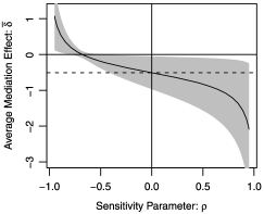
Figure 1: Sensitivity analysis for the media framing experiment. The figure presents the results of the sensitivity analysis described in Section 5. The solid line represents the estimated ACME for the attitude mediator for differing values of the sensitivity parameter $\rho$, which is defined in equation (24). The gray region represents the 95% confidence interval based on the Delta method. The horizontal dashed line is drawn at the point estimate of $\bar{\delta}$ under Assumption 1.

Figure 1 presents the results for the sensitivity analysis based on the residual correlation. We plot the estimated ACME of the attitude mediator against differing values of the sensitivity parameter $\rho$, which is equal to the correlation between the two error terms of equations (27) and (B) for each. The analysis indicates that the original conclusion about the direction of the ACME under Assumption 1 (represented by the dashed horizontal line) would be maintained unless $\rho$ is less than $-0.68$. This implies that the conclusion is plausible given even fairly large departures from the ignorability of the mediator. This result holds even after we take into account the sampling variability, as the confidence interval covers the value of zero only when $-0.79<\rho<-0.49$. Thus, the original finding about the negative ACME is relatively robust to the violation of equation (5) of Assumption 1 under the LSEM.

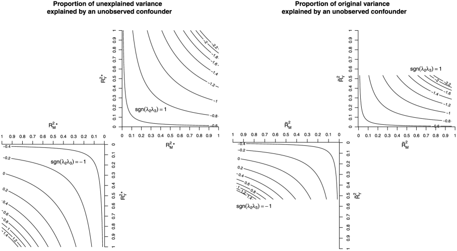
Figure 2: An alternative interpretation of the sensitivity analysis. The plot presents the results of the sensitivity analysis described in Section 5. Each plot contains various mediation effects under an unobserved pre-treatment confounder of various magnitudes. The left plot contains the contours for $R^{2*}_{M}$ and $R^{2*}_{Y}$ which represent the proportion of unexplained variance that is explained by the unobserved confounder for the mediator and outcome, respectively. The right plot contains the contours for $\tilde{R}^{2}_{M}$ and $\tilde{R}^{2}_{Y}$ which represent the proportion of the variance explained by the unobserved pre-treatment confounder. Each line represents the estimated ACME under proposed values of either $(R^{*2}_{M},R^{2*}_{Y})$ or $(\tilde{R}^{2}_{M},\tilde{R}^{2}_{Y})$. The term $\operatorname{sgn}(\lambda_{2}\lambda_{3})$ represents the sign on the product of the coefficients of the unobserved confounder.

Next, we present the same sensitivity analysis using the alternative interpretation of $\rho$ which is based on two coefficients of determination as defined in Section 5; (1) the proportion of unexplained variance that is explained by an unobserved pre-treatment confounder ($R^{2*}_{M}$ and $R^{2*}_{Y}$) and (2) the proportion of the original variance explained by the same unobserved confounder ($\tilde{R}^{2}_{M}$ and $\tilde{R}^{2}_{Y}$). Figure 2 shows two plots based on the types of coefficients of determination. The lower left quadrant of each plot in the figure represents the case where the product of the coefficients for the unobserved confounder is negative, while the upper right quadrant represents the case where the product is positive.

For example, this product will be positive if the unobserved pre-treatment confounder represents subjects’ political ideology, since conservatism is likely to be positively correlated with both public order importance and tolerance for the Klan. Under this scenario, the original conclusion about the direction of the ACME is perfectly robust to the violation of sequential ignorability, because the estimated ACME is always negative in the upper right quadrant of each plot. On the other hand, the result is less robust to the existence of an unobserved confounder that has opposite effects on the mediator and outcome. However, even for this alternative situation, the ACME is still guaranteed to be negative as long as the unobserved confounder explains less than 27.7% of the variance in the mediator or outcome that is left unexplained by the treatment alone, no matter how large the corresponding portion of the variance in the other variable may be. Similarly, the direction of the original estimate is maintained if the unobserved confounder explains less than 26.7% (14.7%) of the original variance in the mediator (outcome), regardless of the degree of confounding for the outcome (mediator).

7 Concluding Remarks

In this paper we study identification, inference and sensitivity analysis for causal mediation effects. Causal mediation analysis is routinely conducted in various disciplines, and our paper contributes to this fast-growing methodological literature in several ways. First, we provide a new identification condition for the ACME, which is relatively easy to interpret in substantive terms and also weaker than existing results in some situations. Second, we prove that the estimates based on the standard LSEM can be given valid causal interpretations under our proposed framework. This provides a basis for formally analyzing the validity of empirical studies using the LSEM framework. Third, we propose simple nonparametric estimation strategies for the ACME. This allows researchers to avoid the stronger functional form assumptions required in the standard LSEM. Finally, we offer a parametric sensitivity analysis that can be easily used by applied researchers in order to assess the sensitivity of estimates to the violation of this assumption. We view sensitivity analysis as an essential part of causal mediation analysis because the assumptions required for identifying causal mediation effects are unverifiable and often are not justified in applied settings.

At this point, it is worth briefly considering the progression of mediation research from its roots in the empirical psychology literature to the present. In their seminal paper, Baron and Kenny barokenn86 (1986) supplied applied researchers with a simple method for mediation analysis. This method has quickly gained widespread acceptance in a number of applied fields. While psychologists extended this LSEM framework in a number of ways, little attention was paid to the conditions under which their popular estimator can be given a causal interpretation. Indeed, the formal definition of the concept of causal mediation had to await the later works by epidemiologists and statisticians (Robins and Greenland, (robigree92, 1992); Pearl, (pear01, 2001); Robins, (robi03, 2003)). The progress made on the identification of causal mediation effects by these authors has led to the recent development of alternative and more general estimation strategies (e.g., Imai, Keele and Tingley, (imaikeelting09, 2009); VanderWeele, (vand09, 2009)). In this paper we show that under a set of assumptions this popular product of coefficients estimator can be given a causal interpretation. Thus, over twenty years later, the work of Baron and Kenny has come full circle.

Despite its natural appeal to applied scientists, statisticians often find the concept of causal mediation mysterious (e.g., Rubin, (rubi04, 2004)). Part of this skepticism seems to stem from the concept’s inherent dependence on background scientific theory;whether a variable qualifies as a mediator in a given empirical study relies crucially on the investigator’s belief in the theory being considered. For example, in the social science application introduced in Section 2, the original authors test whether the effect of a media framing on citizens’ opinion about the Klan rally is mediated by a change in attitudes about general issues. Such a setup might make no sense to another political psychologist who hypothesizes that the change in citizens’ opinion about the Klan rally prompts shifts in their attitudes about more general underlying issues. The H1N1 flu virus example mentioned in Section 3.1 also highlights the same fundamental point. Thus, causal mediation analysis can be uncomfortably far from a completely data-oriented approach to scientific investigations. It is, however, precisely this aspect of causal mediation analysis that makes it appealing to those who resist standard statistical analyses that focus on estimating treatment effects, an approach which has been somewhat pejoratively labeled as a “black-box” view of causality (e.g., Skrabanek, (skra94, 1994); Deaton, (deat09, 2009)). It may be the case that causal mediation analysis has the potential to significantly broaden the scope of statistical analysis of causation and build a bridge between scientists and statisticians.

There are a number of possible future generalizations of the proposed methods. First, the sensitivity analysis can potentially be extended to various nonlinear regression models. Some of this has been done by Imai, Keele and Tingley imaikeelting09 (2009). Second, an important generalization would be to allow multiple mediators in the identification analysis. This will be particularly valuable since in many applications researchers aim to test competing hypotheses about alternative causal mechanisms via mediation analysis. For example, the media framing study we analyzed in this paper included another measurement (on a separate group randomly split from the study sample) which was purported to test an alternative causal pathway. The formal treatment of this issue will be a major topic of future research. Third, implications of measurement error in the mediator variable have yet to be analyzed. This represents another important research topic, as mismeasured mediators are quite common, particularly in psychological studies. Fourth, an important limitation of our framework is that it does not allow the presence of a post-treatment variable that confounds the relationship between mediator and outcome. As discussed in Section 3.3, some of the previous results avoid this problem by making additional identification assumptions (e.g., Robins, 2003). The exploration of alternative solutions is also left for future research. Finally, it is important to develop new experimental designs that help identify causal mediation effects with weaker assumptions. Imai, Tingley and Yamamoto imaitingyama09 (2009) present some new ideas on the experimental identification of causal mechanisms.

Appendix A Proof of Theorem 1

First, note that equation (4) in Assumption 1 implies

$$Y_{i}(t^{\prime},m)\mathchoice{\mathrel{\hbox to0.0pt{$\displaystyle\perp$\hss}\mkern 2.0mu{\displaystyle\perp}}}{\mathrel{\hbox to0.0pt{$\textstyle\perp$\hss}\mkern 2.0mu{\textstyle\perp}}}{\mathrel{\hbox to0.0pt{$\scriptstyle\perp$\hss}\mkern 2.0mu{\scriptstyle\perp}}}{\mathrel{\hbox to0.0pt{$\scriptscriptstyle\perp$\hss}\mkern 2.0mu{\scriptscriptstyle\perp}}}T_{i}|M_{i}(t)=m^{\prime},\quad X_{i}=x.$$ (25)

Now, for any $t,t^{\prime}$, we have

$$\quad\mathbb{E}(Y_{i}(t,M_{i}(t^{\prime}))|X_{i}=x)$$

$$\quad\quad=\int\mathbb{E}\bigl{(}Y_{i}(t,m)|M_{i}(t^{\prime})=m,X_{i}=x\bigr{)}$$

$$\quad\hphantom{\quad=\int\,}dF_{M_{i}(t^{\prime})|X_{i}=x}(m)$$

$$\quad\quad=\int\mathbb{E}\bigl{(}Y_{i}(t,m)|M_{i}(t^{\prime})=m,T_{i}=t^{\prime},X_{i}=x\bigr{)}$$

$$\quad\hphantom{\quad=\int\,}dF_{M_{i}(t^{\prime})\mid X_{i}=x}(m)$$

$$\quad\quad=\int\mathbb{E}(Y_{i}(t,m)|T_{i}=t^{\prime},X_{i}=x)$$

$$\quad\hphantom{\quad=\int\,}dF_{M_{i}(t^{\prime})\mid X_{i}=x}(m)$$

$$\quad\quad=\int\mathbb{E}(Y_{i}(t,m)|T_{i}=t,X_{i}=x)$$

$$\quad\hphantom{\quad=\int\,}dF_{M_{i}(t^{\prime})\mid T_{i}=t^{\prime},X_{i}=x}(m)$$

$$\quad\quad=\int\mathbb{E}\bigl{(}Y_{i}(t,m)|M_{i}(t)=m,T_{i}=t,X_{i}=x\bigr{)}$$

$$\quad\hphantom{\quad=\int\,}dF_{M_{i}(t^{\prime})\mid T_{i}=t^{\prime},X_{i}=x}(m)$$

$$\quad\quad=\int\mathbb{E}(Y_{i}|M_{i}=m,T_{i}=t,X_{i}=x)$$

$$\quad\hphantom{\quad=\int\,}dF_{M_{i}(t^{\prime})\mid T_{i}=t^{\prime},X_{i}=x}(m)$$

$$\quad\quad=\int\mathbb{E}(Y_{i}|M_{i}=m,T_{i}=t,X_{i}=x)$$ (26)

$$\quad\hphantom{\quad=\int\,}dF_{M_{i}\mid T_{i}=t^{\prime},X_{i}=x}(m),$$

where the second equality follows from equation (25), equation (5) is used to establish the third and fifth equalities, equation (4) is used to establish the fourth and last equalities, and the sixth equality follows from the fact that $M_{i}=M_{i}(T_{i})$ and $Y_{i}=Y_{i}(T_{i},M_{i}(T_{i}))$. Finally, equation (A) implies

$$\mathbb{E}(Y_{i}(t,M_{i}(t^{\prime})))$$

$$\quad=\int\int\mathbb{E}(Y_{i}|M_{i}=m,T_{i}=t,X_{i}=x)$$

$$\hphantom{\quad=\int\int\,}dF_{M_{i}\mid T_{i}=t^{\prime},X_{i}=x}(m)\,dF_{X_{i}}(x).$$

Substituting this expression into the definition of $\bar{\delta}(t)$ given by equations (1) and (3.1) yields the desired expression for the ACME. In addition, since $\bar{\tau}=\bar{\zeta}(t)+\bar{\delta}(t^{\prime})$ for any $t,t^{\prime}=0,1$ and $t\neq t^{\prime}$ under Assumption 1, the result for the average natural direct effects is also immediate.

Appendix B Proof of Theorem 2

We first show that under Assumption 1 the model parameters in the LSEM are identified. Rewrite equations (12) and (13) using the potential outcome notation as follows:

$$M_{i}(T_{i}) = \alpha_{2}+\beta_{2}T_{i}+\varepsilon_{i2}(T_{i}),$$ (27)

$$Y_{i}(T_{i},M_{i}(T_{i})) = \alpha_{3}+\beta_{3}T_{i}+\gamma M_{i}(T_{i})$$

$${}+\varepsilon_{i3}(T_{i},M_{i}(T_{i})),$$

where the following normalization is used: $\mathbb{E}(\varepsilon_{i2}(t))=\mathbb{E}(\varepsilon_{i3}(t,m))=0$ for $t=0,1$ and $m\in\mathcal{M}$. Then, equation (4) of Assumption 1 implies $\varepsilon_{i2}(t)\mathchoice{\mathrel{\hbox to0.0pt{$\displaystyle\perp$\hss}\mkern 2.0mu{\displaystyle\perp}}}{\mathrel{\hbox to0.0pt{$\textstyle\perp$\hss}\mkern 2.0mu{\textstyle\perp}}}{\mathrel{\hbox to0.0pt{$\scriptstyle\perp$\hss}\mkern 2.0mu{\scriptstyle\perp}}}{\mathrel{\hbox to0.0pt{$\scriptscriptstyle\perp$\hss}\mkern 2.0mu{\scriptscriptstyle\perp}}}T_{i}$, yielding $\mathbb{E}(\varepsilon_{i2}(T_{i})|T_{i}=t)=\mathbb{E}(\varepsilon_{i2}(t))=0$ for any $t=0,1$. Similarly, equation (5) implies $\varepsilon_{i3}(t,m)\mathchoice{\mathrel{\hbox to0.0pt{$\displaystyle\perp$\hss}\mkern 2.0mu{\displaystyle\perp}}}{\mathrel{\hbox to0.0pt{$\textstyle\perp$\hss}\mkern 2.0mu{\textstyle\perp}}}{\mathrel{\hbox to0.0pt{$\scriptstyle\perp$\hss}\mkern 2.0mu{\scriptstyle\perp}}}{\mathrel{\hbox to0.0pt{$\scriptscriptstyle\perp$\hss}\mkern 2.0mu{\scriptscriptstyle\perp}}}M_{i}|T_{i}=t$ for all $t$ and $m$, yielding $\mathbb{E}(\varepsilon_{i3}(T_{i},M_{i}(T_{i}))|T_{i}=t,M_{i}=m)=\mathbb{E}(\varepsilon_{i3}(t,m)|T_{i}=t)=\mathbb{E}(\varepsilon_{i3}(t,m))=0$ for any $t$ and $m$ where the second equality follows from equation (4). Thus, the parameters in equations (12) and (13) are identified under Assumption 1. Finally, under Assumption 1 and the LSEM, we can write $\mathbb{E}(M_{i}|T_{i})=\alpha_{2}+\beta_{2}T_{i}$, and $\mathbb{E}(Y_{i}|M_{i},T_{i})=\alpha_{3}+\beta_{3}T_{i}+\gamma M_{i}$. Using these expressions and Theorem 1, the ACME can be shown to equal $\beta_{2}\gamma$.

Appendix C Proof that $\rho=0$ under Assumption 1

First, as shown in Appendix B, Assumption 1 implies $\mathbb{E}(\varepsilon_{i2}(T_{i})|T_{i})=0$ and $\mathbb{E}(\varepsilon_{i3}(T_{i},M_{i}(T_{i}))|T_{i},\break M_{i})=0$ where the (potential) error terms are defined in equations (27) and (B). These mean independence relationships (together with the law of iterated expectations) imply

$$0 = \mathbb{E}(\varepsilon_{i3}(T_{i},M_{i}(T_{i}))M_{i})$$

$$= \mathbb{E}\bigl{\{}\varepsilon_{i3}(T_{i},M_{i}(T_{i}))\bigl{(}\alpha_{2}+\beta_{2}T_{i}+\varepsilon_{i2}(T_{i})\bigr{)}\bigr{\}}$$

$$= \mathbb{E}\{\varepsilon_{i3}(T_{i},M_{i}(T_{i}))\varepsilon_{i2}(T_{i}))\}.$$

Thus, under Assumption 1, we have $\rho=0\Longleftrightarrow\break\mathbb{E}\{\varepsilon_{i2}(T_{i})\varepsilon_{i3}(T_{i},M_{i}(T_{i}))\}=0$.

Appendix D Proof of Theorem 4

First, we write the LSEM in terms of equations (12) and (3.4). We omit possible pre-treatment confounders $X_{i}$ from the model for notational simplicity, although the result below remains true even if such confounders are included. Since equation (4) implies $\mathbb{E}(\varepsilon_{ji}|T_{i})=0$ for $j=2,3$, we can consistently estimate $(\alpha_{1},\alpha_{2},\beta_{1},\break\beta_{2})$, where $\alpha_{1}=\alpha_{3}+\alpha_{2}\gamma$ and $\beta_{1}=\beta_{3}+\beta_{2}\gamma$, as well as $(\sigma_{1}^{2},\sigma_{2}^{2},\tilde{\rho})$. Thus, given a particular value of $\rho$, we have $\tilde{\rho}\sigma_{1}\sigma_{2}=\gamma\sigma_{2}^{2}+\rho\sigma_{2}\sigma_{3}$ and $\sigma_{1}^{2}=\gamma^{2}\sigma_{2}^{2}+\sigma_{3}^{2}+2\gamma\rho\sigma_{2}\sigma_{3}$. If $\rho=0$, then $\gamma=\tilde{\rho}\sigma_{1}/\sigma_{2}$ provided that $\sigma_{3}^{2}=\sigma_{1}^{2}(1-\tilde{\rho}^{2})\geq 0$. Now, assume $\rho\neq 0$. Then, substituting $\sigma_{3}=(\tilde{\rho}\sigma_{1}-\gamma\sigma_{2})/\rho$ into the above expression of $\sigma_{1}^{2}$ yields the following quadratic equation: $\gamma^{2}-2\gamma\tilde{\rho}\sigma_{1}/\sigma_{2}+\sigma_{1}^{2}(\tilde{\rho}^{2}-\rho^{2})/\{\sigma_{2}^{2}(1-\rho^{2})\}=0$. Solving this equation and using $\sigma_{3}\geq 0$, we obtain the following desired expression: $\gamma=\frac{\sigma_{1}}{\sigma_{2}}\{\tilde{\rho}-\rho\sqrt{(1-\tilde{\rho}^{2})/(1-\rho^{2})}\}$. Thus, given a particular value of $\rho$, $\bar{\delta}(t)$ is identified.

Appendix E Nonparametric Sensitivity Analysis

We consider a sensitivity analysis for the simple plug-in nonparametric estimator introduced in Section 4.2. Unfortunately, sensitivity analysis is not as straightforward as the parametric settings. Here, we examine the special case of binary mediator and outcome where some progress can be made and leave the development of sensitivity analysis in a more general nonparametric case for future research.

We begin by the nonparametric bounds on the ACME without assuming equation (5) of the sequential ignorability assumption. In the case of binary mediator and outcome, we can derive the following sharp bounds using the result of sjol09 (2009):

$$\max\left\{\begin{array}[]{l}-P_{001}-P_{011}\\ -P_{000}-P_{001}-P_{100}\\ -P_{011}-P_{010}-P_{110}\end{array}\right\}$$ (32)

(33)

$$\quad\leq\bar{\delta}(1)\leq\min\left\{\begin{array}[]{l}P_{101}+P_{111}\\ P_{000}+P_{100}+P_{101}\\ P_{010}+P_{110}+P_{111}\end{array}\right\},$$ (37)

$$\max\left\{\begin{array}[]{l}-P_{100}-P_{110}\\ -P_{001}-P_{100}-P_{101}\\ -P_{110}-P_{011}-P_{111}\end{array}\right\}$$ (41)

(42)

$$\quad\leq\bar{\delta}(0)\leq\min\left\{\begin{array}[]{l}P_{000}+P_{010}\\ P_{010}+P_{011}+P_{111}\\ P_{000}+P_{001}+P_{101}\end{array}\right\},$$ (46)

where $P_{ymt}\equiv\Pr(Y_{i}=y,M_{i}=m|T_{i}=t)$ for all $y,m,\break t\in\{0,1\}$. These bounds always contain zero, implying that the sign of the ACME is not identified without an additional assumption even in this special case.

To construct a sensitivity analysis, we follow the strategy of Imai and Yamamoto imaiyama10 (2010) and first express the second assumption of sequential ignorability using the potential outcomes notation as follows:

$$\quad\Pr\bigl{(}Y_{i}(1,1)=y_{11},Y_{i}(1,0)=y_{10},$$

$$\quad\phantom{\Pr(}Y_{i}(0,1)=y_{01},Y_{i}(0,0)=y_{00}|M_{i}=1,T_{i}=t^{\prime}\bigr{)}$$

$$\quad\quad=\Pr\bigl{(}Y_{i}(1,1)=y_{11},Y_{i}(1,0)=y_{10},$$ (47)

$$\quad\phantom{\quad=\Pr(}Y_{i}(0,1)=y_{01},Y_{i}(0,0)=y_{00}|$$

$$\quad\hskip 4.0pt\phantom{\quad=\Pr(Y_{i}(1,1)=y_{11}}M_{i}=0,T_{i}=t^{\prime}\bigr{)}$$

for all $t^{\prime},y_{tm},\in\{0,1\}$. The equality states that within each treatment group the mediator is assigned independent of potential outcomes. We now consider the following sensitivity parameter $\upsilon$, which is the maximum possible difference between the left- and right-hand side of equation (E). That is, $\upsilon$ represents the upper bound on the absolute difference in the proportion of any principal stratum that may exist between those who take different values of the mediator given the same treatment status. Thus, this provides one way to parametrize the maximum degree to which the sequential ignorability can be violated. (Other, potentially more intuitive, parametrization are possible, but, as shown below, this parametrization allows for easier computation of the bounds.)

Using the population proportion of each principal stratum, that is, $\pi_{y_{11}y_{10}y_{01}y_{00}}^{m_{1}m_{0}}\equiv\Pr(Y_{i}(1,1)=y_{11},\break Y_{i}(1,0)=y_{10},Y_{i}(0,1)=y_{01},Y_{i}(0,0)=y_{00},M_{i}(1)=\break m_{1},M_{i}(0)=m_{0})$, we can write this difference as follows:

$$\hskip 10.0pt\biggl{|}\frac{\sum_{m_{0}=0}^{1}\pi^{1m_{0}}_{y_{11}y_{10}y_{01}y_{00}}}{\sum_{y=0}^{1}P_{y11}}-\frac{\sum_{m_{0}=0}^{1}\pi^{0m_{0}}_{y_{11}y_{10}y_{01}y_{00}}}{\sum_{y=0}^{1}P_{y01}}\biggr{|}$$

(48)

$$\hskip 10.0pt\quad\leq\upsilon,$$

$$\hskip 10.0pt\biggl{|}\frac{\sum_{m_{1}=0}^{1}\pi^{m_{1}1}_{y_{11}y_{10}y_{01}y_{00}}}{\sum_{y=0}^{1}P_{y10}}-\frac{\sum_{m_{1}=0}^{1}\pi^{m_{1}0}_{y_{11}y_{10}y_{01}y_{00}}}{\sum_{y=0}^{1}P_{y00}}\biggr{|}$$

(49)

$$\hskip 10.0pt\quad\leq\upsilon,$$

where $\upsilon$ is bounded between $0$ and $1$. Clearly, if and only if $\upsilon=0$, the sequential ignorability assumption is satisfied.

Finally, note that the ACME can be written as the following linear function of unknown parameters $\pi_{y_{11}y_{10}y_{01}y_{00}}^{m_{1}m_{0}}$:

$$\bar{\delta}(t) = \sum_{m=0}^{1}\sum_{y_{1-t,m}=0}^{1}\sum_{y_{1,1-m}=0}^{1}\sum_{y_{0,1-m}=0}^{1}$$

$$\Biggl{(}\sum_{m_{0}=0}^{1}\pi_{y_{11}y_{10}y_{01}y_{00}}^{mm_{0}}-\sum_{m_{1}=0}^{1}\pi_{y_{11}y_{10}y_{01}y_{00}}^{m_{1}m}\Biggr{)},$$

where one of the subscripts of $\pi$ corresponding to $y_{tm}$ is equal to $1$. Then, given a fixed value of sensitivity parameter $\upsilon$, you can obtain the sharp bounds on the ACME by numerically solving the linear optimization problem with the linear constraints implied by equations (E) and (E) as well as the following relationship implied by the ignorability of the treatment assignment:

$$P_{ymt}=\sum_{y_{1-t,m}=0}^{1}\sum_{y_{t,1-m}=0}^{1}\sum_{y_{1-t,1-m}=0}^{1}\sum_{m_{1-t}=0}^{1}\pi_{y_{11}y_{10}y_{01}y_{00}}^{m_{1}m_{0}}$$ (51)

for each $y,m,t\in\{0,1\}$. In addition, we use the linear constraint that all $\pi_{y_{11}y_{10}y_{01}y_{00}}^{m_{1}m_{0}}$ sum up to $1$.

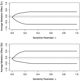
Figure 3: Nonparametric sensitivity analysis for the media framing experiment. In each panel the solid curves show the sharp upper and lower bounds on the ACME as a function of the sensitivity parameter $\upsilon$, which represents the degree of violation of the sequential ignorability assumption. The horizontal dashed lines represent the point estimates of $\bar{\delta}(1)$ (upper panel) and $\bar{\delta}(0)$ (lower panel) under Assumption 1. In contrast to the parametric sensitivity analysis reported in Section 6.2, the estimates are shown to be rather sensitive to the violation of Assumption 1.

We apply this framework to the media framing example described in Sections 2 and 6. For the purpose of illustration, we dichotomize both the mediator and treatment variables using their sample medians as cutpoints. Figure 3 shows the results of this analysis. In each panel the solid curves represent the sharp upper and lower bounds on the ACME for different values of the sensitivity parameter $\upsilon$. The horizontal dashed lines represent the point estimates of $\bar{\delta}(1)$ (upper panel) and $\bar{\delta}(0)$ (lower panel) under Assumption 1. This corresponds to the case where the sensitivity parameter is exactly equal to zero (i.e., $\upsilon=0$), so that equation (E) holds. The sharp bounds widen as we increase the value of $\upsilon$, until they flatten out and become equal to the no-assumption bounds given in equations (32) and (41).

The results suggest that the point estimates of the ACME are rather sensitive to the violation of the sequential ignorability assumption. For both $\bar{\delta}(1)$ and $\bar{\delta}(0)$, the upper bounds sharply increase as we increase the value of $\upsilon$ and cross the zero line at small values of $\upsilon$ [$0.019$ for $\bar{\delta}(1)$ and $0.022$ for $\bar{\delta}(0)$]. This contrasts with the parametric sensitivity analyses reported in Section 6.2, where the estimates of the ACME appeared quite robust to the violation of Assumption 1. Although the direct comparison is difficult because of different parametrization and variable coding, this stark difference illustrates the potential importance of parametric assumptions in causal mediation analysis; a significant part of identification power could in fact be attributed to such functional form assumptions as opposed to empirical evidence.

References

- (1) Albert, J. M. (2008). Mediation analysis via potential outcomes models. Stat. Med. 27 1282–1304. \MR2420158
- (2) Angrist, J. D., Imbens, G. W. and Rubin, D. B. (1996). Identification of causal effects using instrumental variables (with discussion). J. Amer. Statist. Assoc. 91 444–455.
- (3) Avin, C., Shpitser, I. and Pearl, J. (2005). Identifiability of path-specific effects. In Proceedings of the International Joint Conference on Artificial Intelligence. Morgan Kaufman, San Francisco, CA. \MR2192340
- (4) Baron, R. M. and Kenny, D. A. (1986). The moderator–mediator variable distinction in social psychological research: Conceptual, strategic, and statistical considerations. Journal of Personality and Social Psychology 51 1173–1182.
- (5) Cochran, W. G. (1957). Analysis of covariance: Its nature and uses. Biometrics 13 261–281. \MR0090952
- (6) Deaton, A. (2009). Instruments of development: Randomization in the tropics, and the search for the elusive keys to economic development. Proc. Br. Acad. 162 123–160.
- (7) Egleston, B., Scharfstein, D. O., Munoz, B. and West, S. (2006). Investigating mediation when counterfactuals are not metaphysical: Does sunlight UVB exposure mediate the effect of eyeglasses on cataracts? Working Paper 113, Dept. Biostatistics, Johns Hopkins Univ., Baltimore, MD.
- (8) Elliott, M. R., Raghunathan, T. E. and Li, Y. (2010). Bayesian inference for causal mediation effects using principal stratification with dichotomous mediators and outcomes. Biostatistics. 11 353–372.
- (9) Gallop, R., Small, D. S., Lin, J. Y., Elliot, M. R., Joffe, M. and Ten Have, T. R. (2009). Mediation analysis with principal stratification. Stat. Med. 28 1108–1130.
- (10) Geneletti, S. (2007). Identifying direct and indirect effects in a non-counterfactual framework. J. Roy. Statist. Soc. Ser. B 69 199–215. \MR2325272
- (11) Glynn, A. N. (2010). The product and difference fallacies for indirect effects. Unpublished manuscript, Dept. Government, Harvard Univ.
- (12) Goodman, L. A. (1960). On the exact variance of products. J. Amer. Statist. Assoc. 55 708–713. \MR0117809
- (13) Green, D. P., Ha, S. E. and Bullock, J. G. (2010). Yes, but what’s the mechanism? (don’t expect an easy answer). Journal of Personality and Social Psychology 98 550–558.
- (14) Hafeman, D. M. and Schwartz, S. (2009). Opening the black box: A motivation for the assessment of mediation. International Journal of Epidemiology 38 838–845.
- (15) Hafeman, D. M. and VanderWeele, T. J. (2010). Alternative assumptions for the identification of direct and indirect effects. Epidemiology 21. To appear.
- (16) Imai, K. and Yamamoto, T. (2010). Causal inference with differential measurement error: Nonparametric identification and sensitivity analysis. American Journal of Political Science 54 543–560.
- (17) Imai, K., Keele, L. and Tingley, D. (2009). A general approach to causal mediation analysis. Psychological Methods. To appear.
- (18) Imai, K., Keele, L., Tingley, D. and Yamamoto, T. (2010). Causal mediation analysis using R. In Advances in Social Science Research Using R (H. D. Vinod, ed.). Lecture Notes in Statist. 196 129–154. Springer, New York.
- (19) Imai, K., Keele, L. and Yamamoto, T. (2010). Replication data for: Identification, inference, and sensitivity analysis for causal mediation effects. Available at http://hdl.handle.net/1902.1/14412.
- (20) Imai, K., Tingley, D. and Yamamoto, T. (2009). Experimental designs for identifying causal mechanisms. Technical report, Dept. Politics, Princeton Univ. Available at http://imai.princeton.edu/research/Design.html.
- (21) Imbens, G. W. (2003). Sensitivity to exogeneity assumptions in program evaluation. American Economic Review 93 126–132.
- (22) Jo, B. (2008). Causal inference in randomized experiments with mediational processes. Psychological Methods 13 314–336.
- (23) Joffe, M. M., Small, D., Ten Have, T., Brunelli, S. and Feldman, H. I. (2008). Extended instrumental variables estimation for overall effects. Int. J. Biostat. 4 Article 4. \MR2399287
- (24) Joffe, M. M., Small, D. and Hsu, C.-Y. (2007). Defining and estimating intervention effects for groups that will develop an auxiliary outcome. Statist. Sci. 22 74–97. \MR2408662
- (25) Judd, C. M. and Kenny, D. A. (1981). Process analysis: Estimating mediation in treatment evaluations. Evaluation Review 5 602–619.
- (26) Kraemer, H. C., Kiernan, M., Essex, M. and Kupfer, D. J. (2008). How and why criteria definig moderators and mediators differ between the Baron & Kenny and MacArthur approaches. Health Psychology 27 S101–S108.
- (27) Kraemer, H. C., Wilson, T., Fairburn, C. G. and Agras, W. S. (2002). Mediators and moderators of treatment effects in randomized clinical trials. Archives of General Psychiatry 59 877–883.
- (28) MacKinnon, D. P. (2008). Introduction to Statistical Mediation Analysis. Taylor & Francis, New York.
- (29) Nelson, T. E., Clawson, R. A. and Oxley, Z. M. (1997). Media framing of a civil liberties conflict and its effect on tolerance. American Political Science Review 91 567–583.
- (30) Pearl, J. (2001). Direct and indirect effects. In Proceedings of the Seventeenth Conference on Uncertainty in Artificial Intelligence (J. S. Breese and D. Koller, eds.) 411–420. Morgan Kaufman, San Francisco, CA.
- (31) Pearl, J. (2010). An introduction to causal inference. Int. J. Biostat. 6 Article 7.
- (32) Petersen, M. L., Sinisi, S. E. and van der Laan, M. J. (2006). Estimation of direct causal effects. Epidemiology 17 276–284.
- (33) Robins, J. (1999). Marginal structural models versus structural nested models as tools for causal inference. In Statistical Models in Epidemiology, the Environment and Clinical Trials (M. E. Halloran and D. A. Berry, eds.) 95–134. Springer, New York. \MR1731682
- (34) Robins, J. M. (2003). Semantics of causal DAG models and the identification of direct and indirect effects. In Highly Structured Stochastic Systems (P. J. Green, N. L. Hjort and S. Richardson, eds.) 70–81. Oxford Univ. Press, Oxford. \MR2082403
- (35) Robins, J. M. and Greenland, S. (1992). Identifiability and exchangeability for direct and indirect effects. Epidemiology 3 143–155.
- (36) Roy, J., Hogan, J. W. and Marcus, B. H. (2008). Principal stratification with predictors of compliance for randomized trials with 2 active treatments. Biostatistics 9 277–289.
- (37) Rubin, D. B. (2004). Direct and indirect causal effects via potential outcomes (with discussion). Scand. J. Statist. 31 161–170. \MR2066246
- (38) Rubin, D. B. (2005). Causal inference using potential outcomes: Design, modeling, decisions. J. Amer. Statist. Assoc. 100 322–331. \MR2166071
- (39) Sjölander, A. (2009). Bounds on natural direct effects in the presence of confounded intermediate variables. Stat. Med. 28 558–571.
- (40) Skrabanek, P. (1994). The emptiness of the black box. Epidemiology 5 5553–5555.
- (41) Sobel, M. E. (1982). Asymptotic confidence intervals for indirect effects in structural equation models. Sociological Methodology 13 290–321.
- (42) Sobel, M. E. (2008). Identification of causal parameters in randomized studies with mediating variables. Journal of Educational and Behavioral Statistics 33 230–251.
- (43) Ten Have, T. R., Joffe, M. M., Lynch, K. G., Brown, G. K., Maisto, S. A. and Beck, A. T. (2007). Causal mediation analyses with rank preserving models. Biometrics 63 926–934. \MR2395813
- (44) VanderWeele, T. J. (2008). Simple relations between principal stratification and direct and indirect effects. Statist. Probab. Lett. 78 2957–2962.
- (45) VanderWeele, T. J. (2009). Marginal structural models for the estimation of direct and indirect effects. Epidemiology 20 18–26.
- (46) VanderWeele, T. J. (2010). Bias formulas for sensitivity analysis for direct and indirect effects. Epidemiology. To appear.
- (47) Zellner, A. (1962). An efficient method of estimating seemingly unrelated regressions and tests for aggregation bias. J. Amer. Statist. Assoc. 57 348–368. \MR0139235