Statistical Curse of the Second Half Rank

Abstract

In competitions involving many participants running many races the final rank is determined by the score of each participant, obtained by adding its ranks in each individual race. The “Statistical Curse of the Second Half Rank” is the observation that if the score of a participant is even modestly worse than the middle score, then its final rank will be much worse (that is, much further away from the middle rank) than might have been expected. We give an explanation of this effect for the case of a large number of races using the Central Limit Theorem. We present exact quantitative results in this limit and demonstrate that the score probability distribution will be gaussian with scores packing near the center. We also derive the final rank probability distribution for the case of two races and we present some exact formulae verified by numerical simulations for the case of three races. The variant in which the worst result of each boat is dropped from its final score is also analyzed and solved for the case of two races.

1 Introduction

In competitive individual sports involving many participants it is in some cases standard practice to have several races and determine the final rank for each participant by taking the sum of its ranks in each individual race, thereby defining its score. By comparing the scores of the participants a final rank can be decided among them. Typical examples are regattas, which can involve a large number of sailing boats ($\sim$100), running a somehow large number of consecutive races ($\geq 10$).

An empirical observation of long-time participants is that, if their scores are even slightly below the average, their final rank will be much worse than expected. This frustrating fact, which we may call the “Statistical Curse of the Second Half Rank”, is analyzed in this work and argued to be due to statistical fluctuations in the results of the races, on top of the inherent worth of the participants. Using some simplifying assumptions we demonstrate that it can be explained by a version of the Central Limit Theorem [1, 2] for correlated random variables. A general result for a large number of participants and races is derived. Some exact resuts for a small number of races are presented. A variant of the problem, in which the worst score for each participant is dropped, is also considered and solved for the case of two races.

2 Basic setup

Consider $n_{b}$ boats racing $n_{r}$ races. A boat $i$ in the race $k$ has an individual rank $n_{i,k}\in[1,n_{b}]$ (lower ranks represent better performance). The score of the boat $i$ is the sum $n_{i}=\sum_{k=1}^{n_{r}}n_{i,k}\in[n_{r},n_{r}n_{b}]$ of its individual ranks in each race. The final rank of boat $i$ is determined by the place occupied by its score $n_{i}$ among the scores of the other boats $n_{j}$, with $j\neq i$.

For reasons of simplicity we assume that in a given race the ranks are uniformly distributed random variables with no exaequo (that is, all boats are inherently equally worthy and there are no ties). We shall also take the ranks in different races to be independent random variables. It follows that for the race $k$ the set $\{n_{ik};i=1,2,...,n_{b}\}$ is a random permutation of $\{1,2,...,n_{b}\}$ so that the $n_{i,k}$’s are correlated random variables (in particular $\sum_{i=1}^{n_{b}}n_{i,k}=n_{b}(n_{b}+1)/2$), while $n_{ik}$ and $n_{jk^{\prime}}$ are uncorrelated for $k\neq k^{\prime}$. We are interested in the probability distribution for boat $i$ to have a final rank $m\in[1,n_{b}]$ given its score.

Let us illustrate this situation in the simple case of three boats racing two races. We have to take all random permutations of $\{1,2,3\}$ both for the first and the second race, and to add them to determine the possible scores of the three boats. It is easy to see that for, say, boat $1$ to have a score $n_{1,1}+n_{1,2}=4$ there are twelve possibilities:

i) four instances where $n_{1,1}=1$ and $n_{1,2}=3$,

ii) four instances where $n_{1,1}=2$ and $n_{1,2}=2$, and

iii) four instances where $n_{1,1}=3$ and $n_{1,2}=1$.

In each of these three cases (i), (ii) and (iii), one finds that boat $1$ has an equal probability $1/2$ for its final rank to be either $m=1$ or $m=2$. Its mean rank follows as $\langle m\rangle=1/2(1+2)=3/2$. Clearly the score $4$ is precisely the middle of the set $\{2,3,4,5,6\}$ and $\langle m\rangle=3/2$ is indeed close to the middle rank $2$.

More interestingly, cases (i), (ii) and (iii) give the same final rank probability distribution. It means that the final rank probability distribution depends only on the score of boat $1$, and not on its individual ranks in each of the two races consistent with its score. This fact is particular to two races and would not be true any more for three or more races. The final rank probability distribution for boat $1$ given its score would depend in this case on the full set of its ranks in each race, and not just on its score. The final rank probability distribution should then be defined as the average of the above distributions for all set of ranks consistent with its score.

To avoid this additional averaging and simplify slightly the analysis, we consider from now on $n_{b}$ boats racing $n_{r}$ races, plus an additional virtual boat which is only specified by its score $n_{t}\in[n_{r},n_{r}(n_{b}+1)]$. We are interested in finding the probability distribution for this virtual boat to have a final rank $m\in[1,n_{b}+1]$ given its score $n_{t}$ when it is compared to the set of scores $\{n_{i};i=1,2,...,n_{b}\}$ of the $n_{b}$ boats. By definition this probability distribution will then depend only on three variables: $n_{b}$, the number of boats; $n_{r}$, the number of races; and $n_{t}$, the score of the virtual boat we are interested in.

3 The limit of many races

The problem simplifies when some of the parameters determining the size of the system become large so that we can use central limit-type results. In this section we consider the limit in which the number of races becomes large.

We start with a reminder of the Central Limit Theorem in the case of correlated random variables. Assume $\{x_{i,k};i=1,\dots,n_{b};k=1,2,\dots,n_{r}\}$ to be correlated random variables such that

• they are independent for different $k$,

• the set $\{x_{1,k},x_{2,k},...,x_{n_{b},k}\}$ is distributed according to a joint density probablility distribution which is $k$-independent and whose first two moments (mean and covariance) are $\langle x_{i,k}\rangle=\rho_{i}$ and $\langle x_{i,k}x_{j,k}\rangle-\langle x_{i,k}\rangle\langle x_{j,k}\rangle=\rho_{ij}$.

The CLT states that in the limit $n_{r}\gg 1$ the summed variables $x_{i}=\sum_{k=1}^{n_{r}}x_{i,k}$ are correlated gaussian random variables with $\langle x_{i}\rangle=n_{r}\rho_{i}$ and $\langle x_{i}x_{j}\rangle-\langle x_{i}\rangle\langle x_{j}\rangle=n_{r}\rho_{ij}$, that is, they are distributed in this limit according to the probability density

$$f(x_{1},x_{2},...,x_{n_{b}})=N\exp[-{1\over 2n_{r}}\sum_{i,j}\lambda_{ij}(x_{i}-n_{r}\rho_{i})(x_{j}-n_{r}\rho_{j})]$$ (1)

where $N$ is a normalization constant. The matrix $[\lambda]$ is the inverse of the covariance matrix $[\rho]$, assuming that $[\rho]$ is non-singular.

In the race problem, $x_{i,k}=n_{i,k}$ and $x_{i}=n_{i}$: one has

$$\rho_{i}={n_{b}+1\over 2}$$ (2)

$$\rho_{ii}={n_{b}^{2}-1\over 12}~{},~{}~{}~{}\rho_{ij}=-{n_{b}+1\over 12}~{}~{}(i\neq j)$$ (3)

(off diagonal correlations are negative) so that

$$\rho_{ij}={n_{b}+1\over 12}(n_{b}\delta_{i,j}-1)\quad\quad i,j\in[1,...,n_{b}]$$ (4)

It follows that in the large number of races limit $\langle n_{i}\rangle=n_{r}{n_{b}+1\over 2}$ and $\langle n_{i}n_{j}\rangle-\langle n_{i}\rangle\langle n_{j}\rangle=n_{r}\rho_{ij}$.

The covariance matrix $[\rho]$ is singular with a single zero-eigenvalue eigenvector $(1,1,...,1)$. Any vector perpendicular to $(1,1,...,1)$, that is, such that the sum of its entries is $0$, is an eigenvector with eigenvalue $n_{r}(n_{b}+1)/2$. The fact that $(1,1,...,1)$ is a zero-eigenvalue eigenvector signals that the variable $\sum_{i=1}^{n_{b}}n_{i}=n_{r}n_{b}(n_{b}+1)/2$ is deterministic. It must be “taken out” of the set of the scores before finding the large $n_{r}$ limit. We arrive at the density probability distribution

$$f(n_{1},\dots,n_{n_{b}})=\sqrt{2\pi n_{b}\over\lambda}\left(\sqrt{\lambda\over 2\pi}\right)^{n_{b}}\delta\left(\sum_{i=1}^{n_{b}}n_{i}-{6\over\lambda}\right)\exp\left[-{\lambda\over 2}\sum_{i=1}^{n_{b}}(n_{i}-n_{r}{n_{b}+1\over 2})^{2}\right]$$ (5)

with

$$\lambda={12\over n_{r}n_{b}(n_{b}+1)}$$ (6)

such that indeed $\langle n_{i}\rangle=n_{r}\rho_{i}$ and $\langle n_{i}n_{j}\rangle-\langle n_{i}\rangle\langle n_{j}\rangle=n_{r}\rho_{ij}$.

One can exponentiate the constraint $\delta(\sum_{i=1}^{n_{b}}(n_{i}-n_{r}(n_{b}+1)/2)$ so that

$$f(n_{1},...,n_{n_{b}})=\sqrt{n_{b}\lambda^{n_{b}-1}\over(2\pi)^{n_{b}+1}}\int_{-\infty}^{\infty}\exp\left[-ik\sum_{i=1}^{n_{b}}(n_{i}-n_{r}{n_{b}+1\over 2})-{\lambda\over 2}\sum_{i=1}^{n_{b}}(n_{i}-n_{r}{n_{b}+1\over 2})^{2}\right]dk$$ (7)

For a virtual boat with score $n_{t}$ the probability to have a final rank $m$ is the probability for $m-1$ boats among the $n_{b}$’s to have a score $n_{i}<n_{t}$ and for the other $n_{b}-m+1$’s to have a score $n_{i}\geq n_{t}$

$$P_{n_{t}}(m)={n_{b}\choose m-1}\int_{-\infty}^{n_{t}}dn_{1}\dots dn_{m-1}\int_{n_{t}}^{\infty}dn_{m}\dots dn_{n_{b}}f(n_{1},\dots,n_{n_{b}})$$ (8)

which obviously satisfies $\sum_{m=1}^{n_{b}+1}P_{n_{t}}(m)=1$. It can be rewritten as

$$P_{n_{t}}(m)={n_{b}\choose m-1}\int_{-\infty}^{\infty}w_{n_{t}}(k)^{m-1}(1-w_{n_{t}}(k))^{n_{b}-m+1}\sqrt{n_{b}\over 2\pi\lambda}\exp\left[-{n_{b}k^{2}\over 2\lambda}\right]dk$$ (9)

where

$$w_{n_{t}}(k)=\sqrt{\lambda\over 2\pi}\int_{-\infty}^{n_{t}}\exp\left[-{\lambda\over 2}(n-n_{r}{n_{b}+1\over 2}+{ik\over\lambda})^{2}\right]dn$$ (10)

If we further define

$$\bar{n}_{t}=\sqrt{\lambda}\left(n_{t}-\frac{n_{r}(n_{b}+1)}{2}\right)$$ (11)

and absorb $1/\sqrt{\lambda}$ in $k$, (9) becomes

$$P_{n_{t}}(m)={n_{b}\choose m-1}\int_{-\infty}^{\infty}{w}_{\bar{n}_{t}}(k)^{m-1}(1-{w}_{\bar{n}_{t}}(k))^{n_{b}-m+1}\sqrt{n_{b}\over 2\pi}\exp\left[-{n_{b}{k}^{2}\over 2}\right]d{k}$$ (12)

with

$${w}_{\bar{n}_{t}}(k)=\sqrt{1\over 2\pi}\int_{-\infty}^{\bar{n}_{t}}\exp\left[-\frac{(n+ik)^{2}}{2}\right]dn$$ (13)

The probability distribution (12) is of binomial form but with a $k$-dependent ‘pseudo-probability’ $w_{\bar{n}_{t}}(k)$, and $k$ normally distributed according to $\sqrt{n_{b}/(2\pi)}\exp[-{n_{b}k^{2}/2}]$. We find in particular

$$\langle m\rangle=1+n_{b}\int_{-\infty}^{\infty}{w}_{\bar{n}_{t}}(k)\sqrt{n_{b}\over 2\pi}\exp\left[-{n_{b}{k}^{2}\over 2}\right]d{k}=1+n_{b}\,{\cal{N}}\left(\bar{n}_{t}\sqrt{\frac{n_{b}}{n_{b}-1}}\right)$$ (14)

where ${\cal{N}}(x)$ is the cumulative probability distribution of a normal variable

$${\cal{N}}(x)=\frac{1}{\sqrt{2\pi}}\int_{-\infty}^{x}\exp\left[-\frac{n^{2}}{2}\right]dn$$ (15)

We can go further by considering (12) in the large boat number limit $n_{b}\gg 1$. In this limit, $n_{t}$ scales like $n_{b}$ and thus $\bar{n}_{t}$ is $n_{b}$-independent: the $n_{b}$ dependence of $P_{n_{t}}(m)$ is solely contained in the binomial coefficient and the exponents, not in ${w}_{\bar{n}_{t}}(k)$. Setting $r=m/n_{b}$ (the percentage rank) and using $n!\simeq\sqrt{2\pi n}(n/e)^{n}$ we obtain

$$P_{n_{t}}(r)={1\over\sqrt{2\pi r(1-r)}}\int_{-\infty}^{\infty}\exp\left[-n_{b}\left(r\ln{r\over{w}_{\bar{n}_{t}}(k)}+(1-r)\ln{1-r\over 1-{w}_{\bar{n}_{t}}(k)}+k^{2}/2\right)\right]d{k}$$ (16)

In (16) the exponent of the integrand is negative except when $k=0$ and $r={w}_{\bar{n}_{t}}(k)$: for large $n_{b}$ a saddle point approximation yields that $P_{n_{t}}(r)$ vanishes except when $r$ is taken to be ${w}_{\bar{n}_{t}}(0)$. It follows that the final rank of the virtual boat is essentially fixed by its score $\bar{n}_{t}$

$${\bar{r}}={\cal{N}}({\bar{n}}_{t})$$ (17)

as expected from (13, 14) in the large $n_{b}$ limit and shown in Fig. 1 for $200$ boats racing $30$ races.

Figure 1: The final rank of the virtual boat for $200$ boats racing $30$ races : the continuous line is (17) and the points are numerical simuations for a score $n_{t}$ ranging from $30$ to $6000$ by steps of $500$. Both data in the curve and the simulation points have been divided by $200$. The ”statistical curse (blessing) of the second (first) half rank” effect is clearly visible on the figure.

The fluctuations of $r$ around $\bar{r}$ are obtained by expanding the exponent in (16) around $r=\bar{r}$ (one sets $r\simeq\bar{r}+\epsilon$) and around $k=0$ so that

$$r\ln{r\over{w}_{\bar{n}_{t}}(k)}+(1-r)\ln{1-r\over 1-{w}_{\bar{n}_{t}}(k)}\simeq{(\epsilon-k{w}^{\prime}_{\bar{n}_{t}}(0))^{2}\over 2\bar{r}(1-\bar{r})}$$ (18)

where ${w}^{\prime}_{\bar{n}_{t}}(0)$ is the derivative of ${w}_{\bar{n}_{t}}(k)$ at $k=0$. The integration over $k$ in (16) finally yields

$$P_{n_{t}}(r)={1\over\sqrt{2\pi n_{b}(\bar{r}(1-\bar{r})+{w}^{\prime}_{\bar{n}_{t}}(0)^{2})}}\exp\left[-{n_{b}\epsilon^{2}\over 2(\bar{r}(1-\bar{r})+{w}^{\prime}_{\bar{n}_{t}}(0)^{2})}\right]$$ (19)

which is gaussian distributed around $\epsilon=0$, i.e. $r=\bar{r}$, with variance ${\bar{r}(1-\bar{r})+{w}^{\prime}_{\bar{n}_{t}}(0)^{2}\over n_{b}}$. Since

$${w}^{\prime}_{\bar{n}_{t}}(k)=i\sqrt{1\over 2\pi}\exp\left[-{(i{k}+\bar{n}_{t})^{2}\over 2}\right]$$ (20)

and $\bar{r}={w}_{\bar{n}_{t}}(0)$, $1-\bar{r}=1-{w}_{\bar{n}_{t}}(0)={w}_{-\bar{n}_{t}}(0)$ we eventually get for the variance

$$(\Delta m)^{2}=n_{b}\,\phi(\bar{n}_{t})$$ (21)

In the above we introduced the Kollines function

$$\phi(x)={\cal{N}}(x){\cal{N}}(-x)-{1\over{2\pi}}\exp[-x^{2}]$$ (22)

It is positive, very flat around $x=0$ (the first three derivatives vanish at $x=0$) and is essentially zero when $|x|>3.5$ (see Fig. 2).

Figure 2: The Kollines function

It follows that when $|{n}_{t}-n_{r}(n_{b}+1)/2|\gg 3.5/\sqrt{\lambda}\,(\simeq 3.5n_{b}\sqrt{n_{r}/12})$ the final rank has no fluctuation. It is only when $|{n}_{t}-n_{r}(n_{b}+1)/2|<3.5/\sqrt{\lambda}$ that $\Delta m\simeq\sqrt{n_{b}}$ as illustrated in Fig. 3 for $200$ boats racing $30$ races.

Figure 3: The standard deviation of the final rank of the virtual boat for $200$ boats racing $30$ races : the continuous line is the square root of the Kollines function and the points are numerical simuations for a score $n_{t}$ ranging from $30$ to $6000$ by steps of $500$.

4 Small race number: the case $n_{r}=2$

The problem without the benefit of the large-$n_{r}$ limit becomes harder and, for generic $n_{r}$, is not amenable to an explicit solution. For the case of few races, however, we can obtain exact results.

In the present section we deal with the case $n_{r}=2$, for which we can find the exact solution. Fig. 4 displays the mean final ranks and variances of the virtual boat for $n_{b}=3,4,..,9$ boats racing 2 races. For a given $n_{b}$ the score of the virtual boat spans the interval $[2,2n_{b}+1]$.

Figure 4: By complete enumeration of all permutations: the mean final rank and variance for $3,4,...,9$ boats and $2$ races.

4.1 Sketch and basic properties

For two races, the situation can be sketched by using a $n_{b}\times n_{b}$ square lattice as in Fig. 5 for $n_{b}=6$.

Figure 5: The sketch of an event for $n_{r}=2$ and $n_{b}=6$. A boat is represented by a point whose coordinates are its ranks in the two races. Here, we fix the score $n_{t}=6$ of the virtual boat (dashed diagonal). There are 2 sites occupied in D. Thus, the rank of the virtual boat is $m=3$ for this event.

The two coordinates correspond to the ranks of a boat in each one of the two races. So, each boat will be represented by an occupied site. It follows that each line and each column will be occupied once and only once. This leads to $n_{b}!$ possible configurations.

The score $n_{t}$ of the virtual boat is fixed and represented by the dashed diagonal. Let us call $\bf D$ the domain under the diagonal. The rank of the virtual boat is equal to $m$ when $(m-1)$ sites are occupied in $\bf D$. We have obviously  $P_{n_{t}}(m)=\delta_{m,1}$  when $n_{t}\leq 2$ and  $P_{n_{t}}(m)=\delta_{m,n_{b}+1}$ when $n_{t}\geq 2n_{b}+1$. Moreover, from symmetry considerations,

$$P_{n_{b}+1-k}(m)=P_{n_{b}+2+k}(n_{b}+2-m)\;,\qquad k=0,1,...,n_{b}-1$$ (23)

So, in the following, we will restrict $n_{t}$ to the range $2\leq n_{t}\leq n_{b}+1$. In that case, it is easy to realize that only $(n_{t}-2)$ columns (or lines) are available in D. This implies for $m$ the restriction $1\leq m\leq n_{t}-1$.

We also observe that the distribution is symmetric for $n_{t}=n_{b}+1$ or $n_{b}+2$

$$P_{n_{b}+1}(m)=P_{n_{b}+1}(n_{b}+1-m)=P_{n_{b}+2}(m+1)\;,\qquad m=1,2,...,n_{b}$$ (24)

We will come back to this point later.

4.2 Direct computations of $P_{n_{t}}(m)$ for some $m$

For $m=n_{t}-1$, we observe (see Fig. 6) that there is only one possibility to occupy the $(n_{t}-2)$ sites in D.

Figure 6: A configuration contributing to $P_{n_{t}}(m=n_{t}-1)$. We have only one possibility for the $(n_{t}-2)$ occupied sites under the dashed diagonal.

The $(n_{b}-n_{t}+2)$ remaining occupied sites are distributed randomly on the sites of the $(n_{b}-n_{t}+2)$ remaining lines and columns that are still available. Denoting $(u\equiv n_{b}-n_{t}+2)$ one obtains

$$P_{n_{t}}(m=n_{t}-1)=\frac{u!}{n_{b}!}$$ (25)

Now, for $m=1$, there are no occupied sites in $D$. Let us fill (Fig. 7) the lines, starting from the bottom. On line (a), we have $n_{b}-n_{t}+2$ $(\equiv u)$ available sites; on line (b), we still have $u$ available sites (because of the site occupied in line (a)); and so on, up to line (d). Moreover, from the $u$ upper lines, we still get a factor $u!$.

Figure 7: A configuration contributing to $P_{n_{t}}(1)$. No occupied site belongs to D. For each line a), b), …, d), we have $n_{b}-n_{t}+2$ possibilities for the occupied sites. The remaining occupied sites will generate the factor $P_{n_{t}}(n_{t}-1)$. For further explanations, see the text.

Finally

$$P_{n_{t}}(1)=P_{n_{t}}(n_{t}-1)\cdot\Phi_{1}(u)\qquad\mbox{with}\qquad\Phi_{1}(u)=u^{n_{t}-2}$$ (26)

It is easy to see, from the above considerations, that, for $1\leq m\leq n_{t}-1$

$$P_{n_{t}}(m)=P_{n_{t}}(n_{t}-1)\Phi_{m}(u)$$ (27)

where $\Phi_{m}(u)$ is a polynomial in $u$ with integer values.

For $m=2$, there is one occupied site, $B$, in D.

Figure 8: A configuration contributing to $P_{n_{t}}(2)$. The occupied site, B, in D, has coordinates $i$ and $k$. For further explanations, see the text.

With the coordinates $(i,k)$ defined in Fig. 8, D is the domain $(0\leq i\leq k-1;\;1\leq k\leq n_{t}-2)$ so that

$$P_{n_{t}}(2)=P_{n_{t}}(n_{t}-1).\sum_{{\bf D}}u^{n_{t}-2-k}(u+1)^{k-i-1}u^{i}=P_{n_{t}}(n_{t}-1)\Phi_{2}(u)$$ (28)

with

$$\Phi_{2}(u)=(u+1)^{n_{t}-2}(u+1)-u^{n_{t}-2}(u+n_{t}-1)$$ (29)

The computation for $m=3$ is more involved because the relative position of the two occupied sites in D plays an important role in the expression of the terms to be summed. One gets

$$\Phi_{3}(u) = \frac{1}{2}\bigg{[}(u+2)^{n_{t}-2}(u+1)(u+2)-2(u+1)^{n_{t}-2}(u+1)(u+n_{t}-1)\;+$$ (30)

$$+\;u^{n_{t}-2}(u+n_{t}-1)(u+n_{t}-2)\bigg{]}$$

It is worth noting that, despite the apparent complexity of $\Phi_{3}(u)$, the degree of $\Phi_{m}(u)$ decreases when $m$ increases. We will clarify this point later.

The case $m=4$ seems out of reach by direct computation and will not be pursued along these lines.

4.3 Recursion relation and solution of the case $n_{r}=2$

Looking at (26, 29, 30), we observe that, for $m\leq 2$, $\Phi_{m}(u)$ satisfies the recursion relation

$$\Phi_{m+1}(u)=\frac{1}{m}\bigg{(}(u+1)\Phi_{m}(u+1)-(u+n_{t}-m)\Phi_{m}(u)\bigg{)}$$ (31)

We will now show that (31) holds in general.

Let us write   $P_{n_{t}}(m)=\frac{u!}{n_{b}!}\Phi_{m}(u)=\frac{N(m)}{n_{b}!}$  where $N(m)$ is the number of configurations of the $n_{b}\times n_{b}$ square with $(m-1)$ occupied sites in D. Changing $n_{b}$ into $n_{b}+1$ (which amounts to changing $u$ into $u+1$ while keeping $n_{t}$ unchanged), we call $P^{\prime}_{n_{t}}(m)$ the new probability distribution $P^{\prime}_{n_{t}}(m)=\frac{(u+1)!}{(n_{b}+1)!}\Phi_{m}(u+1)=\frac{N^{\prime}(m)}{(n_{b}+1)!}$  where $N^{\prime}(m)$ is defined like $N(m)$ but for the $(n_{b}+1)\times(n_{b}+1)$ square lattice (Fig. 9).

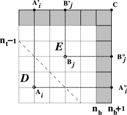
Figure 9: The 3 ways for producing a configuration contributing to $N^{\prime}(m)$ (see the text for definition): i) start from a configuration contributing to $N(m+1)$, erase $A_{i}$ and add $A^{\prime}_{i}$ and $A^{\prime\prime}_{i}$; ii) start from a configuration contributing to $N(m)$, erase $B_{j}$ and add $B^{\prime}_{j}$ and $B^{\prime\prime}_{j}$; iii) start from a configuration contributing to $N(m)$ and add $C$.

$N^{\prime}(m)$ receives three kinds of contributions:

i) Let us consider a configuration contributing to $N(m+1)$ ($m$ occupied sites $A_{i}$ in D – see Fig. 9). The replacement of $A_{i}$ by $A^{\prime}_{i}$ and $A^{\prime\prime}_{i}$ produces a configuration contributing to $N^{\prime}(m)$ (only $(m-1)$ occupied sites in D; all the columns and lines of the biggest square are occupied once). Since we can choose any of the $A_{i}$’s before applying this procedure, we get a contribution $mN(m+1)$ to $N^{\prime}(m)$.

ii) Let us next consider a configuration contributing to $N(m)$ ($n_{b}+1-m$ occupied sites $B_{j}$ in E – see Fig. 9). By the same reasoning as in (i), we get $(n_{b}+1-m)N(m)$ configurations for $N^{\prime}(m)$.

iii) To each configuration contributing to $N(m)$, we can add an occupied site in $C$ (see Fig. 9). This produces the contribution $N(m)$ to $N^{\prime}(m)$.

Summing the above contributions leads to

$$N^{\prime}(m)=mN(m+1)+(n_{b}+2-m)N(m)$$ (32)

Reverting back to $\Phi_{m}$’s, it is straightforward to get (31). Equations (26) and (31) prove that $\Phi_{m}(u)$ has degree $n_{t}-m-1$.

Finally, solving the recursion equation, we get the exact solution for $n_{r}=2$

$$P_{n_{t}}(m)=(n_{b}+1)\sum_{k=0}^{m-1}(-1)^{k}(n_{b}-n_{t}+m-k+1)^{n_{t}-2}\frac{(n_{b}-n_{t}+m-k+1)!}{k!(n_{b}-k+1)!(m-k-1)!}$$ (33)

with  $2\leq m+1\leq n_{t}\leq n_{b}+1$ understood. We have checked (33) by a complete enumeration of the permutations up to $n_{b}$ and $n_{t}=10$.

Let us discuss the case $n_{t}=n_{b}+1$. Equation (33) narrows down to

$$P_{n_{t}}(m)=n_{t}\sum_{k=0}^{m-1}(-1)^{k}\frac{(m-k)^{n_{t}-1}}{k!(n_{t}-k)!}$$ (34)

The moments are

$$\langle m^{n}\rangle = n_{t}\left(\frac{\partial}{\partial\lambda^{\prime}}\right)^{n}\bigg{|}_{\lambda^{\prime}=0}\left(\frac{\partial}{\partial\lambda}\right)^{n_{t}-1}\bigg{|}_{\lambda=0}\sum_{m=1}^{n_{t}-1}\sum_{k=0}^{m-1}\frac{(-1)^{k}}{k!(n_{t}-k)!}e^{\lambda(m-k)}e^{\lambda^{\prime}m}$$ (35)

$$= \frac{1}{(n_{t}-1)!}\left(\frac{\partial}{\partial\lambda^{\prime}}\right)^{n}\bigg{|}_{\lambda^{\prime}=0}\left(\frac{\partial}{\partial\lambda}\right)^{n_{t}-1}\bigg{|}_{\lambda=0}\left[\frac{(1-e^{\lambda^{\prime}})^{n_{t}}-(e^{\lambda+\lambda^{\prime}}-e^{\lambda^{\prime}})^{n_{t}}}{1-e^{\lambda+\lambda^{\prime}}}\right]$$

and in particular

$$\langle m\rangle = \frac{n_{t}}{2}$$ (36)

$$\langle(m-\langle m\rangle)^{2}\rangle = \frac{n_{t}}{12}$$ (37)

$$\langle(m-\langle m\rangle)^{3}\rangle = 0$$ (38)

We recover the fact that $P_{n_{t}}(m)$ is symmetric. These results will be especially useful in the next section.

4.4 Computations of the first three moments for $n_{t}\leq n_{b}$

Starting from the equation (32), we get

$$mP_{n_{t}}(m+1)=(n_{b}+1)P^{\prime}_{n_{t}}(m)-(n_{b}+2-m)P_{n_{t}}(m)$$ (39)

(recall that $P^{\prime}_{n_{t}}(m)$ is the same as $P_{n_{t}}(m)$ but for $n_{b}$ changed into $n_{b}+1$). Multipying both sides of (39) by $m^{k}$ and summing over $m$, the recursion equation for the moments follows

$$(n_{b}+1-k)<m^{k}>+\sum_{p=0}^{k-1}\frac{(-1)^{k+1-p}(k+1)!}{p!(k+1-p)!}<m^{p}>=(n_{b}+1)<m^{k}>^{\prime}$$ (40)

($<...>$ refers to $n_{b}$ and $<...>^{\prime}$ to $n_{b}+1$ ).

For $k=1$, setting $Z_{n_{b}}=n_{b}<m>$, we get $Z_{n_{b}}-Z_{n_{b}-1}=1$ and, finally, $Z_{n_{b}}=Z_{n_{t}-1}+n_{b}-n_{t}+1$. Computing $Z_{n_{t}-1}$ with (36), we obtain the first moment

$$<m>=1+\frac{(n_{t}-1)(n_{t}-2)}{2n_{b}}$$ (41)

The other moments are obtained in a similar way. Equations (37), (38) and (40) lead to:

$$<(m-<m>)^{2}> = \frac{(n_{t}-1)(n_{t}-2)}{12n_{b}^{2}(n_{b}-1)}\left[3n_{t}^{2}-n_{t}(9+8n_{b})+6(n_{b}+1)^{2}\right],\quad n_{b}\geq 2$$ (42)

$$<(m-<m>)^{3}> = \frac{(n_{t}-1)(n_{t}-2)(n_{t}-n_{b}-1)^{2}(n_{t}-n_{b}-2)^{2}}{2n_{b}^{3}(n_{b}-1)(n_{b}-2)}\;,\qquad n_{b}\geq 3$$ (43)

As expected, $<(m-<m>)^{3}>$ vanishes for $n_{t}=n_{b}+1$ or $n_{b}+2$ (the distribution is symmetric); $<(m-<m>)^{2}>$ and $<(m-<m>)^{3}>$ vanish for $n_{t}=1$ or $2$ ($P_{1,2}(m)=\delta_{m,1}$).

5 The case $n_{r}\geq 3$

For the case of three or more races the problem is more complex. We can, however, establish some partial exact results. Fig. 10 demonstrates the stituation for three races, displaying the mean final ranks and variances of the virtual boat for $n_{b}=3,4,5,6$ boats. The score of the virtual boat spans the interval $[3,3n_{b}+1]$.

For $n_{r}=3$ and $n_{t}\leq n_{b}+2$, we established and checked numerically the recursion relation

$$N^{\prime}(m)=(m+1)mN(m+2)+m(2n_{b}-2m+3)N(m+1)+(n_{b}-m+2)^{2}N(m)$$ (44)

More generally, for $n_{r}\geq 3$, we obtained the expression

$$<m>=1+\frac{(n_{t}-1)!}{n_{b}^{n_{r}-1}(n_{t}-1-n_{r})!n_{r}!}\qquad\mbox{for}\qquad n_{r}\leq n_{t}\leq n_{b}+n_{r}-1$$ (45)

Figure 10: By complete enumeration of all permutations: the mean final rank and variance for 3, 4, 5 and 6 boats and 3 races.

6 Two races with the worst individual rank dropped

We conclude our analysis with a variant of the original problem, also used in competitions, for the specific case of two races.

Specifically, suppose that, for each boat, we drop the greatest rank (worst result) obtained in the two races. For instance, if the boat $i$ had ranks $n_{i,1}=2$ and $n_{i,2}=5$, we only retain the score $n_{i}=2$. The virtual boat has a fixed score $n_{t}$ in the range $[1,n_{b}+1]$ and, as before, its rank is $m$ when $(m-1)$ boats have scores $n_{i}$ smaller than $n_{t}$.

It is obvious that $m\geq n_{t}$. Indeed, without loss of generality, we can consider that the ranks $n_{i,1}$ obtained in the first race are arranged in natural order: $\{1,2,...,n_{b}-1,n_{b}\}$, ie $n_{i,1}=i$. (We will keep this order all along this section). Now, from $n_{i}\leq n_{i,1}$, it is easy to realize that, at least $(n_{t}-1)$ boats will have scores $n_{i}$ smaller than $n_{t}$, thus $m\geq n_{t}$.

Defining the ordered sets  $A=\{1,2,...,n_{t}-2,n_{t}-1\}$ and  $B=\{n_{t},n_{t}+1,...,n_{b}-1,n_{b}\}$, we see that, taking, for the ordered set of ranks $r_{i,2}$ in the second race, any permutation of $A$ (for instance $\{n_{t}-2,2,1,...,n_{t}-1\}$ ) followed by any permutation of $B$ (for instance $\{n_{b}-1,n_{t},n_{t}+1,...,n_{b}\}$ ), we construct all the configurations leading to $m=n_{t}$. The number of such configurations is $(n_{t}-1)!\times(n_{b}-n_{t}+1)!$. Dividing by the total number of configurations $n_{b}!$, we get:

$$P_{n_{t}}(n_{t})=\frac{1}{\left(\begin{array}[]{c}n_{b}\\ n_{t}-1\end{array}\right)}$$ (46)

For $m>n_{t}$, we start from the naturally ordered sets $A$ and $B$ and exchange $(m-n_{t})$ elements of $A$ with $(m-n_{t})$ elements of $B$ (of course, $m-n_{t}\leq n_{t}-1$ and $m-n_{t}\leq n_{b}-n_{t}+1$). So, we get the sets $A^{\prime}$ and $B^{\prime}$. Taking, for the ordered set of ranks in the second race, any permutation of $A^{\prime}$ followed by any permutation of $B^{\prime}$, we get all the configurations leading to the rank $m$ for the virtual boat. We eventually obtain a hypergeometric law for the random variable $(m-n_{t})$

$$P_{n_{t}}(m)=\frac{\left(\begin{array}[]{c}n_{t}-1\\ m-n_{t}\end{array}\right)\left(\begin{array}[]{c}n_{b}-n_{t}+1\\ m-n_{t}\end{array}\right)}{\left(\begin{array}[]{c}n_{b}\\ n_{t}-1\end{array}\right)}$$ (47)

with   $n_{t}\leq m\leq\mbox{min}\{2n_{t}-1,\;n_{b}+1\}$

Of course, this probability density is quite different from the one obtained in (33). In particular, it is interesting to note that the distribution (47) is unchanged when we replace, simultaneously,  $n_{t}$ by $n_{t}^{\prime}=n_{b}+2-n_{t}$ and   $m$ by $m^{\prime}=m+n_{b}+2-2n_{t}$

$$P_{n_{t}^{\prime}}(m^{\prime})=P_{n_{t}}(m)$$ (48)

(Note that $n_{t}^{\prime}-1=n_{b}+1-n_{t}$, $n_{b}-n_{t}^{\prime}+1=n_{t}-1$ and $m^{\prime}-n_{t}^{\prime}=m-n_{t}$. So, from (47), $P_{n_{t}}(m)$ is unchanged.)

When $n_{b}$ is even, the distribution is symmetric for $n_{t}=\frac{n_{b}}{2}+1$. Indeed

$$P_{\frac{n_{b}}{2}+1}(m)=\frac{\left(\begin{array}[]{c}\frac{n_{b}}{2}\\ m-\frac{n_{b}}{2}-1\end{array}\right)^{2}}{\left(\begin{array}[]{c}n_{b}\\ \frac{n_{b}}{2}\end{array}\right)}=P_{\frac{n_{b}}{2}+1}\left(\frac{3n_{b}}{2}+2-m\right)\;,\qquad\frac{n_{b}}{2}+1\leq m\leq n_{b}+1$$ (49)

The moments of (47) are

$$<m> = n_{t}+\frac{(n_{t}-1)(n_{b}-n_{t}+1)}{n_{b}}$$ (50)

$$<(m-<m>)^{2}> = \frac{(n_{t}-1)^{2}(n_{b}-n_{t}+1)^{2}}{n_{b}^{2}(n_{b}-1)}\;,\qquad n_{b}\geq 2$$ (51)

$$<(m-<m>)^{3}> = \;-\;\frac{(n_{t}-1)^{2}(n_{b}-n_{t}+1)^{2}(n_{b}-2n_{t}+2)^{2}}{n_{b}^{3}(n_{b}-1)(n_{b}-2)}\;,\qquad n_{b}\geq 3$$ (52)

consistent with (48). Moreover, as expected, $<(m-<m>)^{2}>$ and $<(m-<m>)^{3}>$ vanish for $n_{t}=1$ and $n_{t}=n_{b}+1$. Finally, $<(m-<m>)^{3}>$ vanishes for $n_{t}=\frac{n_{b}}{2}+1$ when $n_{b}$ is even (the distribution is symmetric, see (49)).

7 Conclusions

We demonstrated that the problem of determining the final rank distribution for a boat in a set of races given its total score can be explicitly solved in two distinct situations: for a large number of races, and for a few (2 or 3) races. We also demonstrated that the “Statistical Curse of the Second Half Rank” effect can be attributed to statistical averaging in the case of many races.

Although we obtained our results in the context and language of boat racing, they are clearly applicable in several similar situations, such as, e.g., student ranks based on their results in many exams or quizes, rank of candidates for positions or awards when they are reviewed and ranked by many independent evaluators, and voting results when voters submit a rank of the choices.

There are many open issues and unsolved problems for further investigation. The exact result for an arbitrary number of races (greater than 2) is not known. Further, the obtained results are based on the simplifying assumption that all boats are equally worthy (all ranks in each race are equally probable). One could examine the situation in which boats have a priori different inherent worths, handicapping the probabilities for the ranks, and see to what extent the “statistical curse” effect also emerges. Finally, the relevance and relation of our results with well-known difficulties in rank situations, such as Arrow’s Impossibility theorem [3, 4], would be an interesting topic for further investigation.

Acknowledgements: S.O. acknowledges useful conversations with H.Hilhorst, M. Leborgne, S. Mashkevich and S. Matveenko, and thanks the City College of New York for its hospitality during the completion of this work. A.P. acknowledges the hospitality of CNRS and Université Paris-Sud during the initial stages of this work. The research of A.P. is supported by an NSF grant.

References

• [1] Feller, W. An Introduction to Probability Theory and Its Applications, Vol. 1, 3rd ed. New York: Wiley, p. 229, 1968; Vol. 2, 3rd ed. New York: Wiley, 1971.
• [2] Kallenberg, O. Foundations of Modern Probability. New York: Springer-Verlag, 1997.
• [3] Arrow, K.J. Social choice and individual values. New York: Wiley, 1951
• [4] Geannakoplos, J. Three Brief Proofs of Arrow’s Impossibility Theorem, Economic Theory 26, p. 211, 2005