Generic Conditions for Hydrodynamic Synchronization

Abstract

Synchronization of actively oscillating organelles such as cilia and flagella facilitates self-propulsion of cells and pumping fluid in low Reynolds number environments. To understand the key mechanism behind synchronization induced by hydrodynamic interaction, we study a model of rigid-body rotors making fixed trajectories of arbitrary shape under driving forces that are arbitrary functions of the phases. For a wide class of geometries, we obtain the necessary and sufficient conditions for synchronization of a pair of rotors. We also find a novel synchronized pattern with a time-dependent phase shift. Our results shed light on the role of hydrodynamic interactions in biological systems, and could help in developing efficient mixing and transport strategies in microfluidic devices.

Introduction.

The idea that hydrodynamic interactions at low Reynolds number can induce synchronization between active components with cyclic motion has been the subject of extensive studies since the pioneering work of G. I. Taylor Taylor , and has culminated in a number of direct experimental demonstrations in recent years exp ; Goldstein ; QJ09 . For example, the effective and recovery strokes of beating cilia Blake-Sleigh are considered to be important for generating their coordinated motion (metachrony) GL97 ; KN06 ; GJ07 . While resolving the intricate conformations of the elastic filaments is important for studying coordination in high density assemblies, it can be argued that at sufficiently low densities hydrodynamic interaction does not alter the beating pattern of the active filaments, such that they can be feasibly modeled as simple beads following fixed trajectories VJ06 ; RL06 . The simplicity of this level of description allows for complex many-body effects to be probed in large arrays of such beads with additional active internal mechanisms GJ07 ; LJB03 ; UG10 .

There have been a number of recent studies on hydrodynamic interaction between rotating or orbiting rigid bodies VJ06 ; RL06 ; KP04 ; NEL08 ; RS05 . An emerging general picture suggests that rigid bodies making fixed trajectories do not easily synchronize. Rigid helices with parallel axes KP04 or beads on circular trajectories RL06 with constant driving torque do not synchronize, unless flexibility is introduced in the orientation of the rotation axis RS05 or in the confinement to the trajectory NEL08 , respectively. Vilfan and Jülicher VJ06 studied two beads on tilted elliptic trajectories near a substrate, with a velocity-dependent driving force. They found that both the height-dependence of the drag coefficient and the eccentricity of the trajectories are necessary to stabilize the synchronized state. Ryskin and Lenz RL06 considered a more general model, in which each cilium is represented by a collection of beads connected to each other. Each bead makes a fixed trajectory of arbitrary shape under a driving force that is an arbitrary function of the phase. They applied the general framework to a variety of beating patterns that mimic the ciliary strokes, and found them to be able to stabilize traveling (metachronal) waves but not synchronized states. These results naturally lead to the following question: when do objects with fixed trajectories synchronize via hydrodynamic interaction? Here, we address this question by formulating generic and explicit criteria for hydrodynamic synchronization.

We use a simple version of Ryskin-Lenz model in which each active object (rotor) is made of a single bead. We derive a necessary and sufficient condition for a pair of rotors to synchronize, in terms of the trajectory shape and force profile. We apply the obtained criterion to specific trajectories, and identify the form of the force profiles that cause synchronization. For circular trajectories, for example, we find the requirement that the logarithm of the force has a non-vanishing second-harmonic component of a specific sign, which originates from the second-rank tensorial nature of hydrodynamic interaction. We consider trajectories in the bulk and near a substrate, and those tilted relative to each other. We also develop an effective potential picture to examine the global stability of the synchronized states, which reveals a novel synchronized pattern with a time-dependent phase shift.

Dynamical equations.

We consider a pair of rotors (indexed by $i=1,2$) and assume that each is a spherical bead of radius $a$ that follows a fixed periodic trajectory ${\bf r}_{i}={\bf r}_{i}(\phi_{i})$, where $\phi_{i}=\phi_{i}(t)$ is the phase variable with the period $2\pi$ [see Fig. 1(a)]. The bead is driven by an active force $F_{i}=F_{i}(\phi_{i})$ that is tangential to the orbit and is an arbitrary function of the phase. The hydrodynamic drag force acting on the bead is given by ${\bf g}_{i}=\zeta[{\bf v}({\bf r}_{i})-\dot{\bf r}_{i}]$, where $\zeta=6\pi\eta a$ is the drag coefficient note_on_zeta , and ${\bf v}({\bf r})$ is the velocity field of the surrounding fluid. The tangential component of the drag force is balanced by the driving force acting on each rotor, namely, $F_{i}+{\bf t}_{i}\cdot{\bf g}_{i}=0,$ where ${\bf t}_{i}$ is the tangential unit vector of the orbit given by ${\bf t}_{i}={{\bf r}^{\prime}_{i}}/{|{\bf r}^{\prime}_{i}|}$ with ${\bf r}^{\prime}_{i}={d{\bf r}_{i}}/{d\phi_{i}}$. Substituting the expression for the drag force with $\dot{\bf r}_{i}={\bf r}^{\prime}_{i}\dot{\phi}_{i}$ into the force balance equation, we obtain the phase velocity as $\dot{\phi}_{i}=\omega_{i}+{{\bf t}_{i}\cdot{\bf v}({\bf r}_{i})}/{|{\bf r}^{\prime}_{i}|},$ where $\omega_{i}(\phi_{i})={F_{i}(\phi_{i})}/{\zeta|{\bf r}_{i}^{\prime}|}$ is the intrinsic phase velocity. The reaction force $-{\bf g}_{i}$ exerted by the bead on the fluid generates the flow field

$${\bf v}({\bf r})=-\sum_{j}{\bf G}({\bf r},{\bf r}_{j})\cdot{\bf g}_{j}\simeq\sum_{j}\zeta{\bf G}({\bf r},{\bf r}_{j})\cdot{\bf r}^{\prime}_{j}\omega_{j},$$ (1)

where ${\bf G}({\bf r},{\bf r}_{j})$ is the Oseen tensor describing the hydrodynamic interaction in bulk fluid. On the RHS of Eq. (1), we assumed $|{\bf r}-{\bf r}_{j}|\gg a$ and retained the leading order term with respect to $\zeta{\bf G}({\bf r},{\bf r}_{j})=O(a/|{\bf r}-{\bf r}_{j}|)$. Substituting this into the above expression for the phase velocity, we arrive at the coupled phase oscillator equation

$$\dot{\phi}_{i}=\omega_{i}+\sum_{j\neq i}\left(\frac{{\bf t}_{i}}{|{\bf r}^{\prime}_{i}|}\cdot\zeta{\bf G}_{ij}\cdot|{\bf r}^{\prime}_{j}|{\bf t}_{j}\right)\omega_{j},$$ (2)

where ${\bf G}_{ij}={\bf G}({\bf r}_{i},{\bf r}_{j})$.

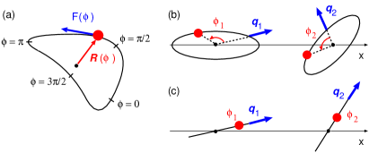
Figure 1: (a) A generic trajectory with its shape specified by ${\bf R}(\phi)$. The bead is driven by the tangential force $F(\phi)$. (b) Circular trajectories ${\bf Q}_{1}\cdot{\bf R}(\phi)$ and ${\bf Q}_{2}\cdot{\bf R}(\phi)$ with ${\bf R}(\phi)=b(\cos\phi,\sin\phi,0)$ and the rotation matrices ${\bf Q}_{1},{\bf Q}_{2}$. Their orientations are specified by the unit vectors ${\bf q}_{i}={\bf Q}_{i}\cdot{\bf e}_{x}$. (c) Linear trajectories with ${\bf R}(\phi)=R(\phi){\bf e}_{x}$ and their orientations specified by ${\bf q}_{i}={\bf Q}_{i}\cdot{\bf e}_{x}$. The centers of the trajectories are both on the $x$-axis.

We now assume that the two trajectories have the same shape but are oriented differently relative to the axis that connects their centers. We can write each trajectory as ${\bf r}_{i}(\phi)={\bf r}_{i0}+{\bf Q}_{i}\cdot{\bf R}(\phi)$, where ${\bf r}_{i0}$ is the position of the center, ${\bf R}(\phi)$ describes the shape of the trajectory, and ${\bf Q}_{i}$ is a rotation matrix. We also assume that the center positions are on the $x$-axis and are separated by the distance $d$ ($\gg a$) from each other, ${\bf r}_{10}=(0,0,0)$ and ${\bf r}_{20}=(d,0,0)$. Using ${\bf r}^{\prime}_{i}(\phi)=|{\bf R}^{\prime}(\phi)|{\bf Q}_{i}\cdot{\bf t}(\phi)$ with the unit vector ${\bf t}(\phi)={\bf R}^{\prime}(\phi)/|{\bf R}^{\prime}(\phi)|$ in Eq. (2), we obtain the difference between the phase velocities as

$$\dot{\phi}_{1}-\dot{\phi}_{2} = \omega(\phi_{1})-\omega(\phi_{2})$$ (3)

$$+ \left[\frac{F(\phi_{2})}{F(\phi_{1})}\omega(\phi_{1})-\frac{F(\phi_{1})}{F(\phi_{2})}\omega(\phi_{2})\right]H(\phi_{1},\phi_{2}),\quad$$

where

$$\omega(\phi_{i})=\frac{F(\phi_{i})}{\zeta|{\bf R}^{\prime}(\phi_{i})|}.$$ (4)

is the intrinsic phase velocity, and we have introduced the coupling function

$$H(\phi_{1},\phi_{2}) = {\bf Q}_{1}\cdot{\bf t}(\phi_{1})\cdot\zeta{\bf G}_{12}\cdot{\bf Q}_{2}\cdot{\bf t}(\phi_{2}),$$ (5)

which is a dimensionless quantity of order $O(a/d)$. To examine the stability of the synchronized state, we set $\phi_{1}=\phi(t)+\delta(t)$, $\phi_{2}=\phi(t)$ and linearize Eq. (3) with respect to the phase difference $\delta(t)$, which gives the linear growth rate

$$\frac{\dot{\delta}}{\delta}=\omega^{\prime}(\phi)+\left[\omega^{\prime}(\phi)-\frac{2F^{\prime}(\phi)}{F(\phi)}\omega(\phi)\right]H(\phi,\phi).$$ (6)

Integrating the above result over the period $T=\int_{0}^{2\pi}d\phi/\dot{\phi}$, we obtain the cycle-averaged growth rate as

$$\Gamma=-\frac{2}{T}\int_{0}^{2\pi}d\phi\,[\ln F(\phi)]^{\prime}H(\phi,\phi),$$ (7)

to the lowest order in the hydrodynamic coupling $H$. A stable synchronized state exists when $\Gamma<0$. Equation (7) thus shows that a necessary condition for synchronization is that both the force profile $F(\phi)$ and the hydrodynamic coupling $H(\phi,\phi)$ are not constant. For any given trajectory ${\bf R}(\phi)$ that gives a non-constant function $H(\phi,\phi)$, we can prescribe a force profile $F(\phi)$ that satisfies the above condition. For example, the force profile $F(\phi)=F_{0}\left[1+\int_{0}^{\phi}d\psi\left(H(\psi,\psi)-\overline{H}\right)\right]$, with $\overline{H}$ being the cycle average of $H(\phi,\phi)$, makes $\Gamma$ negative-definite to the leading order in the coupling.

In order to calculate $H(\phi,\phi)$, we decompose the Oseen tensor into isotropic (I) and dyadic (D) parts as

$$\zeta{\bf G}_{12} = G_{I}(r_{12}){\bf I}+G_{D}(r_{12})\frac{{\bf r}_{12}{\bf r}_{12}}{r_{12}^{2}},$$ (8)

where $G_{I}(r)=G_{D}(r)=3/4r$ and we have used

$${\bf r}_{12}={\bf r}_{1}-{\bf r}_{2}=-d{\bf e}_{x}+{\bf Q}_{1}\cdot{\bf R}(\phi_{1})-{\bf Q}_{2}\cdot{\bf R}(\phi_{2}).\qquad$$ (9)

When the characteristic dimension $b=\max|{\bf R}(\phi)|$ of the trajectory is much smaller than the distance, we can approximate the hydrodynamic interaction kernel as $\zeta G_{12}\simeq G_{I}(d){\bf I}+G_{D}(d){\bf e}_{x}{\bf e}_{x}.$ Under this approximation, the coupling function (5) becomes

$$H(\phi,\phi) = G_{D}(d)\,[{\bf q}_{1}\cdot{\bf t}(\phi)]\,[{\bf q}_{2}\cdot{\bf t}(\phi)]+{\rm const},$$ (10)

where ${\bf q}_{i}={\bf Q}_{i}\cdot{\bf e}_{x}$. Note that the diagonal part of the hydrodynamic kernel gives a constant contribution to $H(\phi,\phi)$ and hence drops off from the integral (7). We now examine a number of cases in more details.

Circular trajectories.

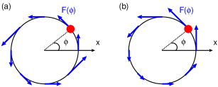
Figure 2: Examples of the force profiles that act to synchronize two beads on circular trajectories aligned on the $x$-axis. (a) $F(\phi)=F_{0}[1-\frac{1}{2}\sin(2\phi)]$. (b) $F(\phi)=F_{0}\left[1+\frac{1}{2}\sin\left(\phi+\frac{\pi}{4}\right)\right]$.

As the first example, let us consider the circular trajectory [see Fig. 1(b)]

$${\bf R}(\phi)=b(\cos\phi,\sin\phi,0).$$ (11)

For this trajectory, we have $|{\bf R}^{\prime}(\phi)|=b$ and ${\bf t}(\phi)=(-\sin\phi,\cos\phi,0)$. First we consider mutually parallel trajectories with ${\bf Q}_{1}={\bf Q}_{2}={\bf I}$. In this case, we have ${\bf q}_{i}={\bf e}_{x}$ and $H(\phi,\phi)=G_{D}(d)\sin^{2}\phi=-\frac{1}{2}G_{D}(d)\cos(2\phi)+{\rm const}$. Note that the factor $\cos 2\phi$ represents the second-rank tensorial nature of the hydrodynamic kernel. To stabilize the synchronized state, we can use the force profile $F(\phi)=F_{0}[1-A\sin(2\phi)]\,(F_{0}>0,0<A<1)$, which gives $\Gamma=-\frac{G_{D}(d)}{T}A+O(A^{2})<0$ [see Fig. 2(a) for illustration]. We can also use $F(\phi)=F_{0}\left[1+B\sin\left(\phi+\frac{\pi}{4}\right)\right]\,(F_{0}>0,-1<B<1)$, which gives $\Gamma=-\frac{G_{D}(d)}{2T}B^{2}+O(B^{4})<0$ [see Fig. 2(b)]. In general, the synchronized state is linearly stable if and only if the Fourier expansion of $\ln F(\phi)$ has a negative coefficient for $\sin 2\phi$.

Next, we consider rotated circular trajectories. For each trajectory ($i=1,2$), the rotation operator that acts on (11) is parameterized by the Euler angles $(\alpha_{i},\beta_{i},\gamma_{i})$ as ${\bf Q}_{i}={\bf M}_{z}(\gamma_{i}){\bf M}_{x}(\beta_{i}){\bf M}_{z}(\alpha_{i}),$ where ${\bf M}_{x}(\theta)$ and ${\bf M}_{z}(\theta)$ are the matrices of rotation by angle $\theta$ around the $x$ and $z$-axis, respectively. It gives ${\bf q}_{i}=(\cos\alpha_{i}\cos\gamma_{i}-\cos\alpha_{i}\cos\beta_{i}\sin\gamma_{i},-\sin\alpha_{i}\cos\gamma_{i}-\cos\alpha_{i}\cos\beta_{i}\cos\gamma_{i},\sin\beta_{i}\sin\gamma_{i}).$ For a rotation in the $xy$-plane ($\beta_{i}=\gamma_{i}=0$), we get $H(\phi,\phi)=-\frac{1}{2}G_{D}(d)\cos(2\phi-\alpha_{1}-\alpha_{2})+{\rm const}.$, and synchronization is induced by, for example, the force profile $F(\phi)=F_{0}[1-A\sin(2\phi-\alpha_{1}-\alpha_{2})]\,(0<A<1)$. Next, a rotation in the $yz$-plane ($\alpha_{i}=\gamma_{i}=0$) gives $H(\phi,\phi)=-\frac{1}{2}G_{D}(d)\cos\beta_{1}\cos\beta_{2}\cos(2\phi)+{\rm const}$. Finally, circular trajectories that are vertical to the $xy$-plane ($\alpha_{i}=0,\beta_{i}=\frac{\pi}{2}$), give $H(\phi,\phi)=-\frac{1}{2}G_{D}(d)\cos\gamma_{1}\cos\gamma_{2}\cos(2\phi)+{\rm const}.$ All of these cases yield similar conditions for synchronization in terms of the second Fourier coefficients of $\ln F(\phi)$, as in the case of non-rotated circular trajectories discussed above. Note that the decay rate to a synchronized state is independent of the size of the trajectory $b$ at the leading order for circular trajectories.

Linear trajectories.

Next we consider the linear trajectory [see Fig. 1(c)]

$${\bf R}(\phi)=R(\phi){\bf e}_{x},$$ (12)

that gives ${\bf t}(\phi)={\rm sgn}[R^{\prime}(\phi)]{\bf e}_{x}$, which amounts to a constant contribution to the coupling function (10) and hence neither stabilize nor destabilize the synchronized state. However, $O(b/d)$ corrections to the hydrodynamic kernel give non-constant contributions. Substituting Eq. (9) into (8) and (5), and retaining the first order term with respect to $R(\phi)$, we obtain the coupling function

$$H(\phi,\phi) = -2R(\phi)\Bigg{[}G_{I}^{\prime}(d)({\bf q}_{1}\cdot{\bf q}_{2})p_{x}+G_{D}^{\prime}(d)q_{1x}q_{2x}p_{x}$$ (13)

$$+ \frac{G_{D}(d)}{d}\left(q_{1x}{\bf q}_{2}\cdot{\bf p}+q_{2x}{\bf q}_{1}\cdot{\bf p}\right)\Bigg{]}+{\rm const},$$

where ${\bf p}={\bf q}_{1}-{\bf q}_{2}$. Note that the coupling is constant when ${\bf q}_{1}={\bf q}_{2}$, because the distance between the two beads is constant when the two trajectories are parallel. When they are not parallel, the phase dependence is proportional to $R(\phi)$. For example, for perpendicular trajectories with ${\bf q}_{1}={\bf e}_{x}$, ${\bf q}_{2}={\bf e}_{y}$ and the orbital profile $R(\phi)=b\cos\phi$, the synchronized state is stabilized if and only if the Fourier expansion of $\ln F(\phi)$ has a positive coefficient for $\sin\phi$.

Nonlinear stability analysis.

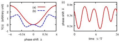
Figure 3: Examples of the effective potential $V(\Delta)$. (a) For the circular trajectory with $F(\phi)=F_{0}[1-\frac{1}{2}\sin(2\phi)]$, the unique stable solution is found at $\Delta=0$. (b) For the elliptic trajectory ${\bf R}(\phi)=b(\cos\phi,\frac{1}{2}\sin\phi,0)$ with $F(\phi)=F_{0}[1-\frac{1}{10}\sin(2\phi)+\frac{1}{2}\sin(4\phi)]$, we obtain the bistable solutions $\Delta=\pm\Delta_{0}$ with $\Delta_{0}\simeq 0.29\pi$, and a metastable solution at $\Delta=\pi$. (c) The stable solution $\Delta=\Delta_{0}$ in (b) gives a time-dependent phase shift $\delta=\delta(t)$ in the original gauge.

We can analyze global stability of the synchronized state by a nonlinear evolution equation for the phase difference. To derive it, first we reparameterize the trajectory by the new phase variable $\Phi=\Phi(\phi)$ that makes the intrinsic phase velocity constant: $\Phi^{\prime}(\phi)\cdot F(\phi)/\zeta|{\bf R}^{\prime}(\phi)|=2\pi/T$. In this gauge, the phase difference $\Delta=\Phi_{1}-\Phi_{2}=\Phi(\phi_{1})-\Phi(\phi_{2})$ obeys [see Eq. (3)]

$$\dot{\Delta}=\frac{2\pi}{T}\left[\frac{\tilde{F}(\Phi_{2})}{\tilde{F}(\Phi_{2}+\Delta)}-\frac{\tilde{F}(\Phi_{2}+\Delta)}{\tilde{F}(\Phi_{2})}\right]\tilde{H}(\Phi_{2}+\Delta,\Phi_{2}),\quad$$ (14)

where $\tilde{F}(\Phi_{2})=F(\phi_{2})$ and $\tilde{H}(\Phi_{1},\Phi_{2})=H(\phi_{1},\phi_{2})$. We now average Eq. (14) over the period $0<t<T$, assuming that $\Delta$ on the RHS is constant over a cycle, which is justified to the leading order in the coupling $H$ Kuramoto . We thus obtain the evolution equation in the form of $\dot{\Delta}=-V^{\prime}(\Delta)$ with an effective potential $V(\Delta)$. The potential is calculated and plotted in Fig. 3 for two examples, which are both non-rotated (${\bf Q}_{i}={\bf I}$) and in the far-field ($d\gg b$). For the circular trajectory, the coupling function $H$ contains only the second harmonic as a function of $\phi$, which results in either the in-phase ($\Delta=0$) or anti-phase ($\Delta=\pi$) synchronization depending on the force profile, as illustrated in Fig. 3(a). For a more complex trajectory like the ellipse, more than one stable and/or metastable solutions can be obtained, as shown in Fig. 3(b). Note that the non-zero values of $\Delta$ generally means non-constant phase shift $\delta=\phi_{1}-\phi_{2}$ in the original gauge, as Fig. 3(c) shows.

Synchronization near a substrate.

Finally, let us consider the case where the rotors are suspended at height $h$ from a flat substrate (located at $z=-h$). In this case, the hydrodynamic coupling is expressed by the Blake tensor Blake , which takes into account the no-slip boundary condition on the substrate. For simplicity, we restrict ourselves to the case where the trajectories are confined in the $xy$-plane and are separated by a relatively large distance, namely $d\gg h,b$. In this case, we can use Eq. (8) with $G_{I}(r)=0$, $G_{D}(r)=9h^{2}/r^{3}$. While all the results discussed above hold true within the above restriction, it is straightforward to extend the analysis to more general and complex geometries.

Discussion.

Our analysis shows that the requirement for hydrodynamic synchronization is nontrivial but not difficult to meet, and that a wide variety of beating patterns do induce synchronization. For the example of circular trajectories, we found that the logarithm of the force should contain second-harmonic component of a specific sign. This can be met if the force profile has the second harmonic directly, or, via frequency doubling, if it has the first harmonic. However, force patterns that only have harmonics higher than two cannot synchronize. Dependences on the trajectory shape and geometry can be summarized by representing the action of a rotor at far distance by force multipoles at a fixed position. For circular orbits, $\Gamma$ is independent of the size of the trajectory, which indicates that the dominant interaction comes from force monopoles when they are in bulk fluid, or dipoles near a substrate (each made of the force monopole and its mirror image Blake ). Linear oscillators do not couple at the first order of the force-multipole expansion. Their leading order coupling comes from the monopole-dipole interaction for beads that are in bulk, or dipole-quadrupole interaction near a substrate. Linear oscillators are also special in the sense that they do not synchronize if they are parallel. This could be relevant to the synchronization of microswimmers PY09 , which can be minimally modeled by a linear configuration of three point forces RG+AA-08 . We have also derived a fully nonlinear evolution equation for the phase difference, which enables us to study the global stability of synchronized states with or without phase shifts. We note that the presence of stable phase shifts has been recently observed in experiments on the beating patterns of the flagella of C. reinhardtii Goldstein . It is not difficult to extend the present analysis to helices (as a model of flagella) or other extended objects to make comparison with experiments.

In conclusion, we have derived a generic and explicit criterion for the trajectory shape and force profile that stabilize synchronized states. The criterion could be helpful in understanding the collective behavior of active biological organelles, and designing active microfluidic components that could be tuned in and out of synchronized states using mechanical signals communicated via hydrodynamic interactions.

- (1) G. I. Taylor, Proc. R. Soc. A 209, 447 (1951). See also: G. J. Elfring and E. Lauga, Phys. Rev. Lett. 103, 088101 (2009).
- (2) M. J. Kim et al., Proc. Natl. Acad. Sci. (USA) 100, 15481 (2003); I. H. Riedel, K. Kruse and J. Howard, Science 309, 300 (2005); J. Kotar et al., Proc. Natl. Acad. Sci. (USA) 107, 7669 (2010).
- (3) M. Polin et al., Science 325, 487 (2009); R. E. Goldstein et al., Phys. Rev. Lett. 103, 168103 (2009).
- (4) B. Qian et al., Phys. Rev. E 80, 061919 (2009).
- (5) J. R. Blake and M. A. Sleigh, Biol. Rev. 49, 85 (1974).
- (6) S. Gueron, K. Levit-Gurevich, N. Liron and J.J. Blum, Proc. Natl. Acad. Sci. (USA) 94, 6001 (1997).
- (7) Y. W. Kim and R. R. Netz, Phys. Rev. Lett. 96, 158101 (2006).
- (8) B. Guirao and J.-F. Joanny, Biophys. J. 92, 1900 (2007).
- (9) A. Vilfan and F. Jülicher, Phys. Rev. Lett. 96, 058102 (2006).
- (10) A. Ryskin and P. Lenz, Phys. Biol. 3, 285 (2006).
- (11) M. Cosentino Lagomarsino, P. Jona and B. Bassetti, Phys. Rev. E 68, 021908 (2003).
- (12) N. Uchida and R. Golestanian, Phys. Rev. Lett. 104, 178103 (2010); Europhys. Lett. 89, 50011 (2010).
- (13) T. Niedermayer, B. Eckhardt, and P. Lenz, Chaos 18, 037128 (2008).
- (14) M. Kim and T.R. Powers, Phys. Rev. E 69, 061910 (2004).
- (15) M. Reichert and H. Stark, Eur. Phys. J. E 17, 493 (2005).
- (16) The drag coefficient is modulated in the presence of the substrate. However, the correction is of and is negligible in our leading order calculations.
- (17) Y. Kuramoto, Chemical Oscillations, Waves, and Turbulence, (Springer, New York, 1984).
- (18) J. R. Blake, Proc. Camb. Phil. Soc. 70, 303 (1971).
- (19) V. B. Putz and J. M. Yeomans, J. Stat. Phys. 137, 1001 (2009).
- (20) R. Golestanian and A. Ajdari, Phys. Rev. E 77, 036308 (2008).