Abstract

A nonperturbative model for the QCD invariant charge, which contains no low–energy unphysical singularities and possesses an elevated higher loop corrections stability, is developed in the framework of potential approach. The static quark–antiquark potential is constructed by making use of the proposed model for the strong running coupling. The obtained result coincides with the perturbative potential at small distances and agrees with relevant lattice simulation data in the nonperturbative physically–relevant region. The developed model yields a reasonable value of the QCD scale parameter, which is consistent with its previous estimations obtained within potential approach.

PACS: 11.15.Tk; 12.38.Aw; 12.39.Pn

Keywords: strong running coupling; potential models

 

1 Introduction

Theoretical description of hadron dynamics at large distances remains a crucial challenge of elementary particle physics for a long time. The asymptotic freedom of Quantum Chromodynamics (QCD) allows one to apply perturbation theory to the study of some “short–range” processes, for example, the high–energy hadronic reactions. However, the study of many phenomena related to the “long–range” dynamics (such as confinement of quarks, structure of the QCD vacuum, etc.) can be performed only within nonperturbative methods.

In general, there is a variety of nonperturbative approaches to handle the strong interaction processes at low energies. For example, one can gain some hints about the hadron dynamics in infrared domain from lattice simulations [1], string models [2], AdS/CFT methods [3, 4], sum rules [5, 6], dispersive (or analytic) approach to QCD [7, 8, 9], bag models [10], potential models [11, 12, 13, 14, 15, 16]. In what follows we shall employ the latter approach, that involves the construction of the QCD invariant charge which satisfies certain nonperturbative requirements.

The objective of this paper is to develop a model for the QCD invariant charge in the framework of potential approach. It is also of a primary interest to apply the proposed model to the construction of the static quark–antiquark potential and compare the obtained result with relevant lattice simulation data.

The layout of the paper is as follows. In Sect. 2 the model for the strong running coupling is formulated and its properties are discussed. Section 3 contains the construction of the potential of quark–antiquark interaction and its comparison with lattice data. In Conclusions (Sect. 4) the obtained results are summarized and further studies within the approach on hand are outlined. Appendix A contains the explicit expressions for the perturbative QCD $\beta$–function and strong running coupling up to the four–loop level. A brief description of the multi–valued Lambert $W$–function is given in App. B.

2 A nonperturbative strong running coupling

As it has been mentioned in the Introduction, the asymptotic freedom enables one to study the strong interaction processes at high energies within perturbative approach. However, the low–energy hadron dynamics entirely remains beyond the applicability range of perturbation theory. In what follows we shall adhere the so–called potential approach [11, 12, 13, 14, 15, 16] to the construction of the nonperturbative model for the QCD invariant charge.

Specifically, in accordance with the basic idea of the potential approach, we shall construct the strong running coupling $\alpha(Q^{2})$ that coincides with perturbative QCD invariant charge in the ultraviolet domain

$$\alpha(Q^{2})\simeq\alpha_{\mbox{\scriptsize pert}}(Q^{2}),\qquad Q^{2}\to\infty,$$ (1)

and meets the requirement of the infrared enhancement

$$\alpha(Q^{2})\simeq\frac{4\pi}{\beta_{0}}\,\frac{\Lambda^{2}}{Q^{2}},\qquad Q^{2}\to 0_{+}.$$ (2)

Here $\alpha_{\mbox{\scriptsize pert}}(Q^{2})$ is the perturbative strong running coupling (see App. A), $\beta_{0}=11-2\,n_{\mbox{\scriptsize f}}/3$ denotes the first coefficient of the $\beta$–function perturbative expansion, $n_{\mbox{\scriptsize f}}$ stands for the number of active quarks, $Q^{2}\geq 0$ is the spacelike momentum transferred, and $\Lambda$ denotes the QCD scale parameter. In terms of the renormalization group $\beta$–function

$$\frac{d\,\ln a(\mu^{2})}{d\,\ln\mu^{2}}=\beta(a)$$ (3)

the conditions (1) and (2) can be equivalently rewritten as

$$\beta(a)\simeq\beta_{\mbox{\scriptsize pert}}(a),\qquad a\to 0_{+},$$ (4)

and

$$\beta(a)\simeq-1,\qquad a\to\infty,$$ (5)

respectively. In these equations $a(Q^{2})\equiv\alpha(Q^{2})\beta_{0}/(4\pi)$ stands for the so–called “couplant”.

One of the possible expressions for the $\beta$–function that satisfies conditions (4) and (5) reads

$$\beta^{(\ell)}(a)=\beta^{(\ell)}_{\mbox{\scriptsize pert}}(a)\,\frac{1-\exp(-2/a)(1-\ell^{2}/B_{\ell-1})}{1+\ell^{2}a^{\ell}},$$ (6)

where $\beta^{(\ell)}_{\mbox{\scriptsize pert}}(a)$ is the $\ell$–loop perturbative QCD $\beta$–function (A.2) and $B_{n}\!=\!\beta_{n}/\beta_{0}^{n+1}$ is the ratio of the $\beta$–function expansion coefficients (see App. A). It is straightforward to verify that at any given loop level $\ell$ the $\beta$–function (6) satisfies the aforementioned condition of linear confinement (5):

$$\beta^{(\ell)}(a)\simeq-1+\frac{C_{\ell}}{a}+{\cal O}\!\left(\frac{1}{a^{2}}\right)\!,\qquad a\to\infty,$$ (7)

where

$$C_{\ell}=\begin{cases}\>1\,,&\quad\ell=1\\[4.2679pt] \displaystyle\>2\!\left(1-\frac{\beta_{\ell-1}}{\ell^{2}\beta_{0}^{\ell}}\right)-\beta_{0}\frac{\beta_{\ell-2}}{\beta_{\ell-1}}\,,&\quad\ell>1\end{cases}$$ (8)

is the combination of the $\beta$–function expansion coefficients. At the same time, for small values of the couplant $a$ the $\beta$–function (6) coincides with the corresponding perturbative result (A.2) up to the uncontrollable at $\ell$–loop level corrections:

$$\beta^{(\ell)}(a)\simeq\beta^{(\ell)}_{\mbox{\scriptsize pert}}(a)+{\cal O}\bigl{(}a^{\ell+1}\bigr{)},\qquad a\to 0_{+}.$$ (9)

Additionally, $\beta$–function (6) admits the explicit integration of the renormalization group equation (3) at the one–loop level and eventually leads to the strong running coupling $\alpha(Q^{2})$ that contains no unphysical singularities at low energies and possesses an elevated stability with respect to the higher loop corrections. The plots of the function $\beta^{(\ell)}(a)$ (6) and the perturbative $\beta$–function (A.2) at $\ell$–loop level ($\ell=1,...,4$) are presented in Figure 1.

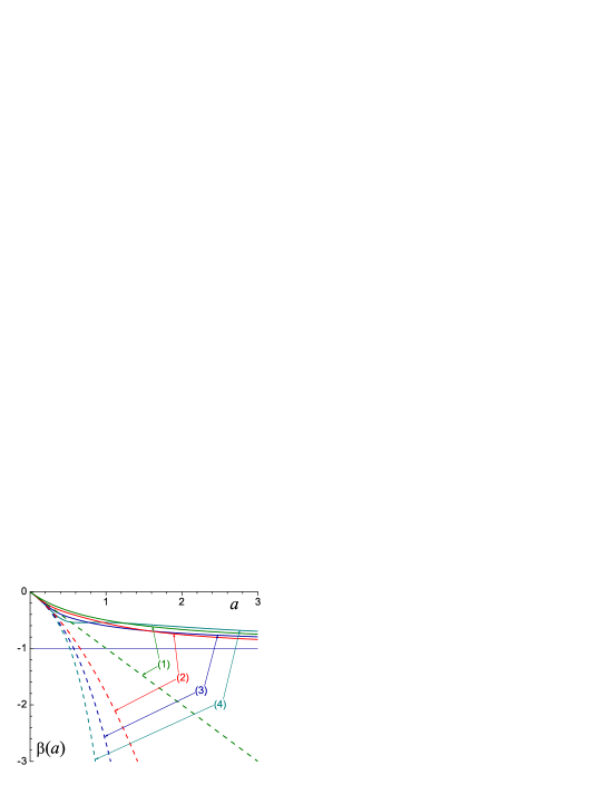
Figure 1: The $\beta$–function $\beta^{(\ell)}(a)$ (6) (solid curves) and the perturbative $\beta$–function $\beta^{(\ell)}_{\mbox{\scriptsize pert}}(a)$ (A.2) (dashed curves). The presented functions correspond to $n_{\mbox{\scriptsize f}}=3$ active quarks. The numerical labels indicate the loop level.

For the beginning, let us consider the one–loop level ($\ell=1$). In this case the $\beta$–function (6) takes a simple form, namely,

$$\beta^{(1)}(a)=-\frac{a}{1+a}.$$ (10)

The corresponding renormalization group equation for the QCD invariant charge $\alpha(Q^{2})$ reads

$$\frac{d\,\ln\bigl{[}a^{(1)}(\mu^{2})\bigr{]}}{d\,\ln\mu^{2}}=-\frac{a^{(1)}(\mu^{2})}{1+a^{(1)}(\mu^{2})}.$$ (11)

After splitting the variables and integrating in finite limits, Eq. (11) takes the following form:

$$\frac{1}{a^{(1)}(Q^{2})}-\ln\Bigl{[}a^{(1)}(Q^{2})\Bigr{]}=\ln\Biggl{(}\frac{Q^{2}}{\Lambda^{2}}\Biggr{)},$$ (12)

where

$$\Lambda^{2}=Q_{0}^{2}\,\frac{\beta_{0}}{4\pi}\,\alpha^{(1)}(Q_{0}^{2})\exp\!\Biggl{[}-\frac{4\pi}{\beta_{0}}\,\frac{1}{\alpha^{(1)}(Q_{0}^{2})}\Biggr{]}$$ (13)

denotes the square of the one–loop scale parameter and $Q_{0}^{2}$ is the normalization point. In turn, Eq. (12) can be solved explicitly in terms of the multi–valued Lambert $W$–function, namely,

$$\alpha^{(1)}(Q^{2})=\frac{4\pi}{\beta_{0}}\,\frac{1}{W_{0}(z)},\qquad z=\frac{Q^{2}}{\Lambda^{2}},$$ (14)

see also Refs. [18, 19]. It is worthwhile to note here that only the principle branch of the Lambert $W$–function, $W_{0}(x)$, is physically meaningful herein. The plots of the couplant corresponding to the invariant charge (14), $a^{(1)}(Q^{2})=1/W_{0}(z)$, and the one–loop perturbative couplant (A.8), $a^{(1)}_{\mbox{\scriptsize pert}}(Q^{2})=1/\ln z$, are presented in Figure 2 (solid and dashed curves labeled “$(1)$”, respectively).

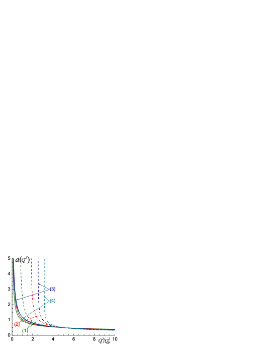
Figure 2: The $\ell$–loop couplant $a^{(\ell)}(Q^{2})$ corresponding to the $\beta$–function (6) (solid curves) and the perturbative couplant $a^{(\ell)}_{\mbox{\scriptsize pert}}(Q^{2})$ (dashed curves). The presented functions are computed for $n_{\mbox{\scriptsize f}}=3$ active quarks and normalized to the value $a(Q^{2})=1/2$ at $Q^{2}=5\,Q_{0}^{2}$. The numerical labels indicate the loop level.

The obtained strong running coupling (14) contains no unphysical singularities in the physical domain $Q^{2}>0$. By making use of the expansions (B.2) and (B.3) one can show that $\alpha^{(1)}(Q^{2})$ (14) possesses the required infrared enhancement,

$$\alpha^{(1)}(Q^{2})\simeq\frac{4\pi}{\beta_{0}}\Biggl{[}\,\frac{1}{z}+1+{\cal O}(z)\Biggr{]},\qquad Q^{2}\to 0_{+},$$ (15)

and tends to the perturbative result (A.8) in the ultraviolet domain,

$$\alpha^{(1)}(Q^{2})\simeq\frac{4\pi}{\beta_{0}}\Biggl{\{}\frac{1}{\ln z}+{\cal O}\!\Biggl{[}\frac{\ln(\ln z)}{\ln^{2}z}\Biggr{]}\!\Biggr{\}},\qquad Q^{2}\to\infty.$$ (16)

It is worth mentioning here that the low–energy behavior of the QCD invariant charge similar to that of Eq. (15) has also been discussed in Refs. [20, 21, 22, 23, 24, 25, 26, 27].

Let us proceed now to the higher loop levels ($\ell>1$). Here, the renormalization group equation (3) with the $\beta$–function (6) can only be integrated numerically. Nonetheless, the asymptotic behavior of the $\ell$–loop QCD invariant charge $\alpha^{(\ell)}(Q^{2})$ corresponding to the $\beta$–function (6) can be found explicitly. Specifically, at any loop level $\alpha^{(\ell)}(Q^{2})$ possesses an enhancement in the infrared asymptotic,

$$\alpha^{(\ell)}(Q^{2})\simeq\frac{4\pi}{\beta_{0}}\Biggl{[}\,\frac{1}{z}+C_{\ell}+{\cal O}(z)\Biggr{]},\qquad Q^{2}\to 0_{+},$$ (17)

and coincides with perturbative strong running coupling $\alpha^{(\ell)}_{\mbox{\scriptsize pert}}(Q^{2})$ (see App. A) in the ultraviolet asymptotic,

$$\alpha^{(\ell)}(Q^{2})\simeq\alpha^{(\ell)}_{\mbox{\scriptsize pert}}(Q^{2})+{\cal O}\!\Biggl{[}\frac{\ln^{\ell}(\ln z)}{\ln^{\ell+1}z}\Biggr{]},\qquad Q^{2}\to\infty.$$ (18)

The constant $C_{\ell}$ in Eq. (17) is defined in Eq. (8). It is worth noting here that the last term of Eq. (18) constitutes a correction, which is not controllable within perturbative approach at the $\ell$–loop level. The plots of the couplants $a^{(\ell)}(Q^{2})$ and $a^{(\ell)}_{\mbox{\scriptsize pert}}(Q^{2})$ at $\ell$–loop level ($\ell=1,...,4$) are presented in Figure 2. As one can infer from this figure, the QCD invariant charge $\alpha^{(\ell)}(Q^{2})$ possesses an elevated (with respect to perturbation theory) higher loop corrections stability in the intermediate energy range. It is worthwhile to note also that the proposed strong running coupling $\alpha(Q^{2})$ is free of low–energy unphysical singularities.

3 Static quark–antiquark potential

Let us address now the construction of the static potential of quark–antiquark interaction $V(r)$. In the framework of potential approach $V(r)$ is related to the strong running coupling $\alpha(Q^{2})$, which satisfies the aforementioned conditions (1) and (2), by the three–dimensional Fourier transformation

$$V(r)=-\frac{16\pi}{3}\int\limits_{0}^{\infty}\frac{\alpha(\bm{Q}^{2})}{\bm{Q}^{2}}\,\frac{\exp(i\bm{Qr})}{(2\pi)^{3}}\,d{\bm{Q}},$$ (19)

see, for example, reviews [14, 15, 16] and references therein. Strictly speaking, this definition of the potential is justified for small distances ($r\lesssim 0.1\,$fm) only. For instance, the lowest–lying bound states of heavy quarks can be described by employing the perturbative QCD [28]. However, at large distances ($r\gtrsim 0.5\,$fm), which play the crucial role in hadron spectroscopy, the perturbative approach becomes inapplicable due to the infrared unphysical singularities (such as the Landau pole) of the strong running coupling $\alpha_{\mbox{\scriptsize pert}}(Q^{2})$. Nonetheless, the potential (19), being constructed with the invariant charge $\alpha(Q^{2})$, which contains no unphysical singularities and satisfies requirements (1) and (2), has proved to be successful in the description of both heavy–quark and light–quark systems (see papers [11, 12, 13] and reviews [14, 15, 16] for the details).

In this paper, for the construction of the static potential of quark–antiquark interaction we shall use the invariant charge (14). After integration over angular variables, Eq. (19) in this case takes the form

$$V(r)=-\frac{32}{3\beta_{0}}\,\Lambda\!\int\limits_{0}^{\infty}\!a(p^{2}\Lambda^{2})\,\frac{\sin(pR)}{pR}\,dp,$$ (20)

where $p=Q/\Lambda$, $R=r\Lambda$, and $a(Q^{2})=1/W_{0}(Q^{2}/\Lambda^{2})$. The integral (20) diverges at the lower limit, that is a common feature of the models of such kind (a detailed discussion of this issue can be found in Sect. 7 and App. C of Ref. [15]). To regularize Eq. (20) it is convenient to split the couplant (14) into singular and regular parts (see also Eq. (15)):

$$a(Q^{2})=a_{1}(z)+a_{2}(z),$$ (21)

where $z=Q^{2}/\Lambda^{2}$ and

$$a_{1}(z)=\frac{1}{z},\qquad a_{2}(z)=\frac{1}{W_{0}(z)}-\frac{1}{z}.$$ (22)

Then, the potential (20) takes the following form:

$$V(r)=\frac{8\pi}{3\beta_{0}}\,\Lambda\biggl{[}U_{1}(R)+U_{2}(R)\biggr{]},$$ (23)

where

$$U_{i}(R)=-\frac{1}{R}\,\frac{4}{\pi}\int\limits_{0}^{\infty}\!a_{i}\Biggl{(}\frac{x^{2}}{R^{2}}\Biggr{)}\frac{\sin x}{x}\,dx,\qquad i=1,2$$ (24)

are the dimensionless parts of the potential and $x=Qr$. The function $U_{1}(R)$ diverges and requires regularization, whereas $U_{2}(R)$ is regular and can be computed numerically.

To regularize function $U_{1}(R)$ we shall employ the method similar to that of used in Ref. [20]. Specifically, in terms of auxiliary function

$$I(t)=\int\limits_{0}^{\infty}x^{t}\sin x\,dx$$ (25)

the singular part of the potential (23) reads

$$U_{1}(R)=-\frac{4}{\pi}\,I(-3)\,R\,.$$ (26)

The integral on the right hand side of Eq. (25) exists for $0\leq|\mbox{Re}\,(t+1)|<1$ (see, for example, Ref. [29]). Nonetheless, Eq. (25) can be analytically continued to the entire complex $t$–plane. This continuation is given by

$$I(t)=\sqrt{\pi}\,2^{t}\,\frac{\Gamma(1+t/2)}{\Gamma\bigl{(}(1-t)/2\bigr{)}}$$ (27)

and plays the role of regularization of Eq. (26), see also Refs. [20, 8]. In this case $I(-3)=-\pi/4$, that results in $U_{1}(R)=R$.

Thus, the static quark–antiquark potential (20) takes the following form:

$$V(r)=V_{0}+\frac{8\pi}{3\beta_{0}}\,\Lambda\Biggl{[}R-\frac{1}{R}\,\frac{4}{\pi}\int\limits_{0}^{\infty}\!a_{2}\Biggl{(}\frac{x^{2}}{R^{2}}\Biggr{)}\frac{\sin x}{x}\,dx\Biggr{]},\qquad R=\Lambda r,$$ (28)

where $V_{0}$ is an additive self–energy constant and $a_{2}(z)$ is given by Eq. (22). At small distances this potential possesses the standard behavior determined by the asymptotic freedom

$$V(r)\simeq\frac{8\pi}{3\beta_{0}}\,\Lambda\,\frac{1}{R\,\ln R},\qquad r\to 0,$$ (29)

whereas at large distances potential (28) proves to be linearly rising

$$V(r)\simeq\frac{8\pi}{3\beta_{0}}\,\Lambda\,R,\qquad r\to\infty,$$ (30)

implying the confinement of quarks. It is straightforward to verify that the potential (28) satisfies also the so–called concavity condition

$$\frac{d\,V(r)}{d\,r}>0,\qquad\frac{d^{2}\,V(r)}{d\,r^{2}}\leq 0,$$ (31)

which is a general property of the gauge theories (see Ref. [30] for the details).

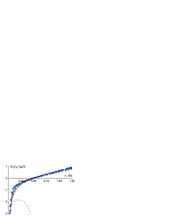
Figure 3: The quark–antiquark potential $V(r)$ (Eq. (28), solid curve) and the lattice simulation data (Ref. [31], symbols “$\bigcirc$”). The Cornell potential [32] is denoted by symbols “$\Box$”, whereas Richardson’s potential [12] is shown by symbols “$\triangle$”. The dashed curve denotes the relevant perturbative result (29). The values of the parameters: $\Lambda=375\,$MeV, $V_{0}=315\,$MeV, $n_{\mbox{\scriptsize f}}=3$.

Figure 3 presents the quark–antiquark potential (28), relevant lattice simulation data [31], Cornell potential [32], and Richardson’s potential [12]. Equation (28) has been fitted to the lattice data [31] by making use of the least square method, $\Lambda$ and $V_{0}$ being the varied parameters. The estimation of the scale parameter in the course of this comparison gives $\Lambda=(375\pm 40)\,$MeV (this value corresponds to the one–loop level with $n_{\mbox{\scriptsize f}}=3$ active quarks). The obtained value of $\Lambda$ agrees with previous estimations [11, 12, 13] of the QCD scale parameter within potential approach. As one can infer from Figure 3, in the region $r\lesssim 0.05\,\mbox{fm}$ the derived potential (28) coincides with the perturbative result (29). At the same time, $V(r)$ (28) is in a good agreement with both Cornell [32] and Richardson’s [12] potentials. Besides, in the nonperturbative physically–relevant range $0.3\,\mbox{fm}\lesssim r\lesssim 1.2\,\mbox{fm}$, in which the average quark separations $\sqrt{\langle r^{2}\rangle}$ for quarkonia sits [34], the obtained potential (28) reproduces the lattice data[31] fairly well.

4 Conclusions

A nonperturbative model for the QCD invariant charge is developed in the framework of potential approach. The proposed strong running coupling is free of low–energy unphysical singularities and embodies the asymptotic freedom with infrared enhancement in a single expression. The model on hand possesses an elevated (with respect to perturbation theory) higher loop corrections stability in the intermediate energy range. The static quark–antiquark potential is constructed by making use of the proposed model for the strong running coupling. The obtained result coincides with the perturbative potential at small distances and agrees with relevant lattice simulation data in the nonperturbative physically–relevant region. The developed model yields a reasonable value of the QCD scale parameter, which agrees with its previous estimations obtained in the framework of potential approach.

In further studies it would undoubtedly be interesting to compute the meson spectrum by making use of the derived quark–antiquark potential as well as to apply the developed model for the QCD invariant charge to the analysis of other strong interaction processes.

Appendix A The QCD $\beta$–function and running coupling
within perturbation theory

The QCD invariant charge $\alpha(Q^{2})$ is the solution of the renormalization group equation

$$\frac{d\,\ln\bigl{[}a(\mu^{2})\bigr{]}}{d\,\ln\mu^{2}}=\beta(a),$$ (A.1)

where $a(Q^{2})\equiv\alpha(Q^{2})\beta_{0}/(4\pi)$ is the so–called “couplant”. For small values of the running coupling the right hand side of Eq. (A.1) is usually approximated by the power series, namely,

$$\beta(a)\simeq\beta^{(\ell)}_{\mbox{\scriptsize pert}}(a)=-\sum_{n=0}^{\ell-1}B_{n}\Bigl{[}a^{(\ell)}_{\mbox{\scriptsize}}(\mu^{2})\Bigr{]}^{n+1},\qquad a\to 0_{+},$$ (A.2)

where $\ell=1,2,3,...$ denotes the loop level and $B_{n}=\beta_{n}/\beta_{0}^{n+1}$ is the ratio of the QCD $\beta$–function perturbative expansion coefficients:

$$\beta_{0} = 11-\frac{2}{3}\,n_{\mbox{\scriptsize f}},$$ (A.3)

$$\beta_{1} = 102-\frac{38}{3}\,n_{\mbox{\scriptsize f}},$$ (A.4)

$$\beta_{2} = \frac{2857}{2}-\frac{5033}{18}\,n_{\mbox{\scriptsize f}}+\frac{325}{54}\,n_{\mbox{\scriptsize f}}^{2},$$ (A.5)

$$\beta_{3} = \frac{149753}{6}+3564\,\zeta(3)-\left[\frac{1078361}{162}+\frac{6508}{27}\,\zeta(3)\right]\!n_{\mbox{\scriptsize f}}$$ (A.6)

$$+\left[\frac{50065}{162}+\frac{6472}{81}\,\zeta(3)\right]\!n_{\mbox{\scriptsize f}}^{2}+\frac{1093}{729}\,n_{\mbox{\scriptsize f}}^{3}.$$

In these equations $n_{\mbox{\scriptsize f}}$ stands for the number of active quarks and $\zeta(x)$ denotes the Riemann $\zeta$–function, $\zeta(3)\simeq 1.202$ (see, for example, Ref. [29]). The one– and two–loop coefficients ($\beta_{0}$ and $\beta_{1}$) are scheme–independent, whereas the expressions given for $\beta_{2}$ and $\beta_{3}$ are calculated in the $\overline{\mbox{MS}}$ subtraction scheme (see papers [35, 36, 37, 38] and references therein for the details). The plots of the $\beta$–function (A.2) are presented in Figure 1 (dashed curves).

The renormalization group equation corresponding to the perturbative $\beta$–function (A.2),

$$\frac{d\,\ln\bigl{[}a^{(\ell)}_{\mbox{\scriptsize pert}}(\mu^{2})\bigr{]}}{d\,\ln\mu^{2}}=\beta^{(\ell)}_{\mbox{\scriptsize pert}}(a),$$ (A.7)

can be solved explicitly at one– and two–loop levels ($\ell=1,2$), namely,

$$a^{(1)}_{\mbox{\scriptsize pert}}(Q^{2}) = \frac{1}{\ln z},\qquad z=\frac{Q^{2}}{\Lambda^{2}},$$ (A.8)

$$a^{(2)}_{\mbox{\scriptsize pert}}(Q^{2}) = -\frac{B_{1}^{-1}}{1+W_{-1}\Bigl{\{}-\exp\Bigl{[}-\bigl{(}1+B_{1}^{-1}\ln z\bigr{)}\Bigr{]}\!\Bigr{\}}}$$ (A.9)

$$\simeq \frac{1}{\ln z}-B_{1}\frac{\ln(\ln z)}{\ln^{2}z},\qquad Q^{2}\to\infty,$$

see also Ref. [39]. In Eq. (A.9) $W_{k}(x)$ stands for the so–called Lambert $W$–function (see App. B for the details). Starting from the three–loop level, the exact solution to the perturbative renormalization group equation (A.7) can not be expressed in terms of known functions. Nonetheless, for $\ell\geq 3$ Eq. (A.7) can be solved iteratively, that eventually leads to

$$a^{(3)}_{\mbox{\scriptsize pert}}(Q^{2}) \simeq \frac{1}{\ln z}-B_{1}\frac{\ln(\ln z)}{\ln^{2}z}$$ (A.10)

$$+\frac{1}{\ln^{3}\!z}\biggl{\{}B_{1}^{2}\Bigl{[}\ln^{2}(\ln z)-\ln(\ln z)-1\Bigr{]}+B_{2}\biggr{\}},$$

$$a^{(4)}_{\mbox{\scriptsize pert}}(Q^{2}) \simeq \frac{1}{\ln z}-B_{1}\frac{\ln(\ln z)}{\ln^{2}z}$$ (A.11)

$$+\frac{1}{\ln^{3}\!z}\biggl{\{}B_{1}^{2}\Bigl{[}\ln^{2}(\ln z)-\ln(\ln z)-1\Bigr{]}+B_{2}\biggr{\}}$$

$$+\frac{1}{\ln^{4}\!z}\Biggl{\{}B_{1}^{3}\biggl{[}-\ln^{3}(\ln z)+\frac{5}{2}\ln^{2}(\ln z)$$

$$+2\ln(\ln z)-\frac{1}{2}\biggr{]}-3B_{1}B_{2}\ln(\ln z)+\frac{1}{2}B_{3}\Biggr{\}}.\hskip 14.22636pt$$

It is worth noting here that the presented in Figure 2 plots of the $\ell$–loop perturbative couplant $a^{(\ell)}_{\mbox{\scriptsize pert}}(Q^{2})$ (dashed curves) correspond to exact solutions of the renormalization group equation (A.7).

Appendix B The Lambert $W$–function

The Lambert $W$–function is defined as the multi–valued function $W_{k}(x)$, which satisfies the equation

$$W_{k}(x)\exp\Bigl{[}W_{k}(x)\Bigr{]}=x,$$ (B.1)

where $k$ denotes the branch index. Only two branches of this function, namely, $W_{0}(x)$ (the principal branch) and $W_{-1}(x)$, take real values (see Figure 4), whereas the other branches take imaginary values. For the branches $W_{0}(x)$ and $W_{-1}(x)$ of the Lambert $W$–function the following expansions hold:

$$W_{0}(x) = \ln x-\ln(\ln x)+{\cal O}\!\Biggl{[}\frac{\ln(\ln x)}{\ln x}\Biggr{]},\qquad x\to\infty,\qquad~{}$$ (B.2)

$$W_{0}(x) = x-x^{2}+{\cal O}(x^{3}),\qquad x\to 0,$$ (B.3)

$$W_{-1}(-x) = \ln x+{\cal O}\bigl{(}\ln|\ln x|\bigr{)},\qquad x\to 0_{+},$$ (B.4)

$$W_{-1}\left(-\frac{1}{e}+x\right) = -1-\sqrt{2\,e\,x}+{\cal O}(x),\qquad x\to 0_{+},$$ (B.5)

where $e\simeq 2.71828$ denotes the base of natural logarithm. The detailed description of the Lambert $W$–function and its properties can be found in Ref. [17].

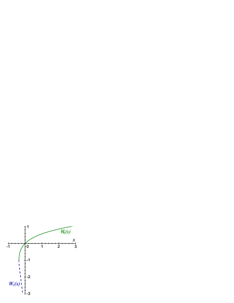
Figure 4: Two real branches of the Lambert $W$–function (B.1): $W_{0}(x)$ (solid curve) and $W_{-1}(x)$ (dashed curve).

References

- [1] G.S. Bali, Phys. Rept. 343, 1 (2001); H.J. Rothe, World Sci. Lect. Notes Phys. 74, 1 (2005); C. Gattringer and C.B. Lang, Lect. Notes Phys. 788, 1 (2010).
- [2] B.M. Barbashov and V.V. Nesterenko, Introduction to the Relativistic String Theory (World Scientific, Singapore, 264 p., 1990).
- [3] J. Erlich, E. Katz, D.T. Son, and M.A. Stephanov, Phys. Rev. Lett. 95, 261602 (2005); J. Erlich, Int. J. Mod. Phys. A 25, 411 (2010).
- [4] O. Andreev and V.I. Zakharov, Phys. Rev. D 74, 025023 (2006); S.J. Brodsky, Eur. Phys. J. A 31, 638 (2007); C.D. White, Phys. Lett. B 652, 79 (2007).
- [5] M.A. Shifman, A.I. Vainshtein, and V.I. Zakharov, Nucl. Phys. B 147, 385 (1979); 147, 448 (1979).
- [6] L.J. Reinders, H. Rubinstein, and S. Yazaki, Phys. Rept. 127, 1 (1985); S. Narison, Nucl. Phys. B (Proc. Suppl.) 164, 225 (2007); 207, 315 (2010).
- [7] D.V. Shirkov and I.L. Solovtsov, Theor. Math. Phys. 150, 132 (2007) [Teor. Mat. Fiz. 150, 152 (2007)].
- [8] A.V. Nesterenko, Int. J. Mod. Phys. A 18, 5475 (2003).
- [9] G. Cvetic and C. Valenzuela, Braz. J. Phys. 38, 371 (2008).
- [10] P. Hasenfratz and J. Kuti, Phys. Rept. 40, 75 (1978); C.E. DeTar and J.F. Donoghue, Ann. Rev. Nucl. Part. Sci. 33, 235 (1983); S.L. Adler and T. Piran, Rev. Mod. Phys. 56, 1 (1984).
- [11] W. Celmaster and F.S. Henyey, Phys. Rev. D 18, 1688 (1978); R. Levine and Y. Tomozawa, ibid. 19, 1572 (1979); 21, 840 (1980).
- [12] J.L. Richardson, Phys. Lett. B 82, 272 (1979).
- [13] W. Buchmuller, G. Grunberg, and S.-H. H. Tye, Phys. Rev. Lett. 45, 103 (1980); 45, 587(E) (1980); W. Buchmuller and S.-H. H. Tye, Phys. Rev. D 24, 132 (1981).
- [14] A.A. Bykov, I.M. Dremin, and A.V. Leonidov, Sov. Phys. Usp. 27, 321 (1984) [Usp. Fiz. Nauk 143, 3 (1984)]; A.W. Hendry and D.B. Lichtenberg, Fortsch. Phys. 33, 139 (1985); J.H. Kuhn and P.M. Zerwas, Phys. Rept. 167, 321 (1988).
- [15] W. Lucha, F.F. Schoberl, and D. Gromes, Phys. Rept. 200, 127 (1991).
- [16] W. Lucha and F.F. Schoberl, arXiv:hep-ph/9601263; N. Brambilla and A. Vairo, arXiv:hep-ph/9904330.
- [17] R.M. Corless, G.H. Gonnet, D.E.G. Hare, D.J. Jeffrey, and D.E. Knuth, Adv. Comput. Math. 5, 329 (1996); D.J. Jeffrey, D.E.G. Hare, and R.M. Corless, Math. Scient. 21, 1 (1996).
- [18] Yu.O. Belyakova, Proc. Int. Conf. Lomonosov–2009 (Moscow, Russia, 2009), ed. N.N. Sysoev (Moscow State University, 2009), p. 215.
- [19] Yu.O. Belyakova, Proc. Int. Conf. Lomonosov–2010 (Moscow, Russia, 2010), ed. N.N. Sysoev (Moscow State University, 2010), Vol. 2, p. 155.
- [20] A.V. Nesterenko, Phys. Rev. D 62, 094028 (2000); 64, 116009 (2001).
- [21] A.V. Nesterenko, Nucl. Phys. B (Proc. Suppl.) 133, 59 (2004); Int. J. Mod. Phys. A 19, 3471 (2004).
- [22] A.V. Nesterenko, Proc. 4th Int. Conf. on Quark Confinement and the Hadron Spectrum (Vienna, Austria, 2000), eds. W. Lucha and K.M. Maung (World Scientific, Singapore, 2002), p. 255; arXiv:hep-ph/0010257.
- [23] A.V. Nesterenko, Proc. 5th Int. Conf. on Quark Confinement and the Hadron Spectrum (Gargnano, Italy, 2002), eds. N. Brambilla and G. Prosperi (World Scientific, Singapore, 2003), p. 288; arXiv:hep-ph/0210122.
- [24] A.C. Aguilar, A.V. Nesterenko, and J. Papavassiliou, J. Phys. G 31, 997 (2005).
- [25] A.I. Alekseev and B.A. Arbuzov, Mod. Phys. Lett. A 13, 1747 (1998); 20, 103 (2005); Phys. Atom. Nucl. 61, 264 (1998) [Yad. Fiz. 61, 314 (1998)].
- [26] P.A. Raczka, Nucl. Phys. B (Proc. Suppl.) 164, 211 (2007); arXiv:hep-ph/0602085; arXiv:hep-ph/0608196.
- [27] V.V. Kiselev, A.E. Kovalsky, and A.I. Onishchenko, Phys. Rev. D 64, 054009 (2001).
- [28] S. Titard and F.J. Yndurain, Phys. Rev. D 49, 6007 (1994); 51, 6348 (1995).
- [29] I.S. Gradshteyn and I.M. Ryzhik, Table of Integrals, Series, and Products, 7th edn., (Academic Press, Amsterdam, Boston, 1171 p., 2007).
- [30] E. Seiler, Phys. Rev. D 18, 482 (1978); C. Bachas, ibid. 33, 2723 (1986).
- [31] G.S. Bali et al., (SESAM and TL Collaborations), Phys. Rev. D 62, 054503 (2000).
- [32] E. Eichten, K. Gottfried, T. Kinoshita, J.B. Kogut, K.D. Lane, and T.M. Yan, Phys. Rev. Lett. 34, 369 (1975); 36, 1276(E) (1976); E. Eichten, K. Gottfried, T. Kinoshita, K.D. Lane, and T.M. Yan, Phys. Rev. D 17, 3090 (1978); 21, 313(E) (1980); 21, 203 (1980).
- [33] M. Peter, Phys. Rev. Lett. 78, 602 (1997); Nucl. Phys. B 501, 471 (1997); K. Hagiwara, A.D. Martin, and A.W. Peacock, Z. Phys. C 33, 135 (1986).
- [34] G.S. Bali, K. Schilling, and A. Wachter, Phys. Rev. D 56, 2566 (1997); G.S. Bali and P. Boyle, ibid. 59, 114504 (1999).
- [35] D.J. Gross and F. Wilczek, Phys. Rev. Lett. 30, 1343 (1973); H.D. Politzer, ibid. 30, 1346 (1973).
- [36] W.E. Caswell, Phys. Rev. Lett. 33, 244 (1974); D.R.T. Jones, Nucl. Phys. B 75, 531 (1974); E. Egorian and O.V. Tarasov, Theor. Math. Phys. 41, 863 (1979) [Teor. Mat. Fiz. 41, 26 (1979)].
- [37] O.V. Tarasov, A.A. Vladimirov, and A.Yu. Zharkov, Phys. Lett. B 93, 429 (1980); S.A. Larin and J.A.M. Vermaseren, ibid. 303, 334 (1993).
- [38] T. van Ritbergen, J.A.M. Vermaseren, and S.A. Larin, Phys. Lett. B 400, 379 (1997); K.G. Chetyrkin, B.A. Kniehl, and M. Steinhauser, Phys. Rev. Lett. 79, 2184 (1997).
- [39] E. Gardi, G. Grunberg, and M. Karliner, JHEP 9807, 007 (1998); B.A. Magradze, arXiv:hep-ph/9808247.