Cosmographic applications of Gamma Ray Bursts

Abstract

In this work we present some applications about the use of the so-called Cosmography with GRBs. In particular, we try to calibrate the Amati relation by using the luminosity distance obtained from the cosmographic analysis. Thus, we analyze the possibility of use GRBs as possible estimators for the cosmological parameters, obtaining as preliminary results a good estimate of the cosmological density parameters, just by using a GRB data sample.

1 Introduction

It is a matter of fact that Gamma Ray Bursts (GRBs) are the most powerful explosions in the Universe; this feature makes them as one of the most studied objects in high energy astrophysics. The flux observed from their emission and the measurement of the redshift $z$ from the observations of the afterglow [Costa et al.(1997)], point out a very high value for the isotropic energy emitted in the burst, so that there are some GRBs observed at very high redshift. Up to date, the farthest GRB has a spectroscopic redshift of $\sim$ 8.2 [Tanvir et al.(2009), Salvaterra et al.(2009)]. These interesting features suggest a possible use of GRBs as distance indicators; unfortunately our knowledge on the mechanisms underlying the GRB emission is not completely understood, so that their use as standard candles is still not clear. However, there exist some correlations among the observed spectroscopic and photometric properties of the GRBs, allowing us to put severe constraints on the GRBs distances. What we need is an independent estimation of the isotropic energy $E_{iso}$ emitted from a GRB. Indeed, by using the GRB’s fluence $S_{obs}$ measured by a detector in a certain energy range, it becomes possible to determine the luminosity distance $d_{l}$ as follows

$$d_{l}=\left(\frac{E_{iso}(1+z)}{S_{bolo}}\right)^{\frac{1}{2}},$$ (1)

where $S_{bolo}$ is the bolometric fluence emitted, obtained from the Schaefer formula [Schaefer(2007)]

$$S_{bol}=S_{obs}\frac{\int_{1/(1+z)}^{10^{4}/(1+z)}E\phi dE}{\int_{E_{min}}^{E^{max}}E\phi dE}.$$ (2)

In literature there are many correlation formulas, each of them takes in account different observed quantities, but in this work we assume the validity of the so-called Amati relation [Amati et al.(2002)], for different reasons

1

it relates just the isotropic energy with the peak energy in the $\nu$F($\nu$) spectrum without considering others,

2

it involves time-independent quantities, overcoming the problem of the large instrumental biases,

3

all of the long GRBs satisfy the Amati relation, while the same is not true for the other correlations.

In addition, although the Amati relation suffers of some biases, as the detector dependence of the observed quantity considered [Shahmoradi & Nemiroff(2009), Butler et al.(2009)], it seems to be well verified from observations [Amati et al.(2009)]. However, one of the most relevant challenge is represented by the calibration of the Amati relation, because a low redshift sample of GRBs is, up to now, lacking; a similar sample should be necessary in order to allow us to calibrate the relation too as well as the Supernovae Ia (SNeIa) calibration procedure. Anyway, a first computation of the relation parameters has been performed by considering the concordance model, namely the Lambda-Cold Dark Matter ($\Lambda$CDM), obtaining a model-dependent luminosity distance. Unfortunately this procedure leads naturally to the so-called circularity problem when we take into account a cosmological use of the GRBs with the Amati relation. A possible solution has been provided by the use of SNeIa [Perlmutter et al.(1999)]. In other words, one can wonder if it is possible to calibrate GRBs by adopting at low redshift the SNeIa sample. This proposal has been already developed in literature by [Liang et al.(2008)]. On the other hand, recently it has been investigated an alternative to solve this controversy, by adopting a model-independent procedure described by Cosmography, which shall be clarified in the next section.

2 The cosmographic Amati relation

As stressed above, the necessity to account a procedure which is based on a model-independent way for characterizing the Universe dynamics is essential; indeed, different cosmological tests may be taken into account; unfortunately for any case, one of the major difficulty is related to choosing which may be considered the less model independent one. One of these, first discussed by Weinberg [Weinberg(1972)] and recently by Visser [Visser(2004)], proposes to consider the waste amount of kinematical quantities as constraints to discriminate if a model works well or not. Cosmography is exactly what we mean for that; we refer to it as the part of cosmology trying to infer the kinematical quantities as the expansion velocity, the deceleration parameter and so on, just making the minimal assumption of a Friedman-Robertson-Walker (FRW) metrics, being $ds^{2}=c^{2}dt^{2}-a(t)^{2}\big{[}dr^{2}+r^{2}\left(\sin^{2}\theta d\theta^{2}+d\phi^{2}\right)\big{]}$, [Weinberg(1972)]; in particular, it is based only on keeping the geometry by assuming the Taylor expansion of the scale factor $a(t)$. In this way we do not do predictions about the standard Hubble law, but only about its kinematical constraints; it is worth noting that once expanded as a Taylor series the Hubble law it is consequent to expand the luminosity distance $d_{l}$ too and then the distance modulus $\mu(z)$ [Capozziello & Izzo(2010)]; unfortunately it is clear that a similar expansion diverges for $z>1$. Thus to circumvent this mathematical issue it should be necessary to change the variable, defining conventionally

$$y=\frac{z}{1+z},$$ (3)

which limits the redshift range, i.e. $y$ $\in$ (0,1). With this model-independent formulation we can immediately determine the cosmographic parameters, in order to reconstruct the trend of the function $d_{l}$(y) also at high redshift. Indeed, our aim consists in assuming the luminosity distance obtained with a good distance indicators, (SNeIa), extending it also for high redshifts. So far, as a first step we estimated the cosmographic parameters from a very large sample of SNeIa, by adopting the Union 2 compilation [Amanullah et al.(2010))]; to perform this, we used a likelihood function $L$ $\propto$ $e^{-\chi^{2}/2}$, where the chi-squared, $\chi^{2}$ is given by

$$\chi^{2}=\sum_{i}\frac{(\mu(y)-\mu_{i})^{2}}{\sigma_{\mu_{i}}^{2}},$$ (4)

where $\mu_{i}$ are the distance modulus for each Union SNeIa and $\sigma\mu_{i}$ its correspondent error. The results are summarized in Table 1.

Once having an expression for $d_{l}$, in principle, it would be possible to calibrate the Amati relation too, by using the observed redshift and the bolometric fluence $S_{bolo}$ of a GRB, computing the isotropic energy, by inverting eq. 1. Then, having as the Amati relation $E_{iso}$ = $A$ $E_{p,i}^{\gamma}$, we evaluated the parameters $A$ and $\gamma$, through the use of a sample of 108 GRBs [Capozziello & Izzo(2010)], considering as estimator a log-likelihood function and taking into account the possible existence of an extra variability $\sigma_{ext}$ of the $y$ data, due to some hidden variables that we cannot observe directly [D’Agostini(2005)]. The cosmographic calibration gives as results the following values

$$A=49.17\pm 0.40,\hskip 28.45274pt\gamma=1.46\pm 0.29,$$ (5)

and in Fig. 1 the best fit curve in the E_p – E_iso plane is showed.

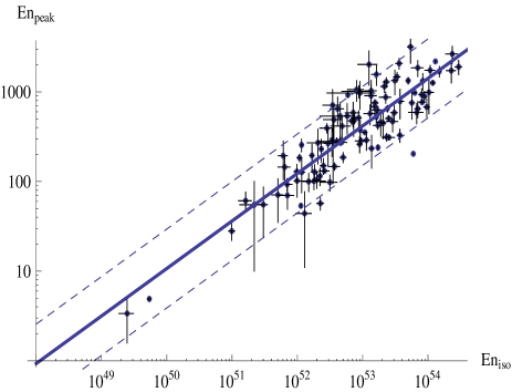
Figure 1: Plot of the cosmographic Amati relation in the E_p – E_iso one. The line of prediction bounds represents a deviation of 2$\sigma_{ext}$ from the best fit line, the thick one.

Table 1: Cosmographic parameters obtained using the SneIa sample Union 2. Note that we have considered for the determination of the jerk $j_{0}$ and of the snap $s_{0}$ the flatness condition $\Omega_{k}$ = 0. The error on $s_{0}$ does not include the contribute from covariance terms and the dimension of $H_{0}$ are $km\,(sMpc)^{-1}$.

Parameter	value	error
H0	$69.90$	$0.027$
q0	$-0.58$	$0.03$
j0	$1.50$	$0.22$
s0	$-2.96$	$1.58$

3 Cosmological applications

Although of its elegance, our calibration of the Amati relation has been obtained using a formulation of $d_{l}$ which suffers from some theoretical misleading problems. First of all, since it is defined for low values of the redshift, the consequent extension to higher redshift may bring to deviations from the real cosmological picture. In order to check this discrepancy, we plotted in fig. 2 both the distance modulus obtained from Cosmography by SNeIa and from a flat $\Lambda$CDM paradigm, with $\Omega_{\rho}=0.27$, being the matter density. We immediately note a difference of one magnitude at redshift z $\approx 4$, increasing with $z$, due to different possible reasons

1

the propagation of the systematics in the analysis of the SNeIa used for calibration,

2

the large scatter in the data sample of the Amati relation,

3

the standard $\Lambda$CDM model fails at high redshift.

The latter assumption seems to be the less probable one, since the $\Lambda$CDM model is able to explain the growing of structure formations too. In addition, in the following, we are going to present a cosmological application of the GRB sample to estimate the density parameters.

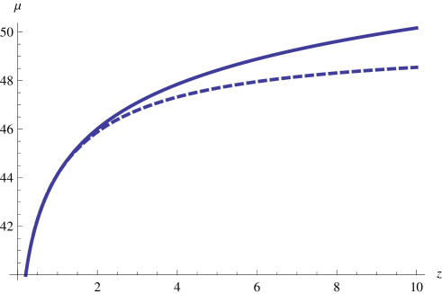
Figure 2: Plot of the $\mu$(y) computed for a fiducial $\Lambda$CDM cosmological model, the continuous line, and for the reconstructed $\mu$(y) obtained from the cosmographic fit of the SneIa, the dashed line, in function of the z redshift.

Let us first compute the isotropic energy E_iso for each GRB from the cosmographic Amati relation, obtaining the distance modulus for each of them, by using the bolometric fluence S_bolo of eq. (2). Thus, the GRB sample becomes related to the following theoretical distance modulus

$$D_{L}(z)=\frac{c}{H_{0}}{1+z\over\sqrt{|\Omega_{k}|}}\textrm{sinn}\Big{(}\sqrt{|\Omega_{k}|}\int_{0}^{z}{d\xi\over E(\xi)}\Big{)}\,,$$ (6)

with $E(z)$ the reduced Hubble parameter, i.e. $E\equiv\frac{H(z)}{H_{0}}$, while $\Omega_{k}$ represents the fractional curvature density at $z=0$, and

$${\textrm{sinn}(x)}=\left\{\begin{array}[]{ll}{\textrm{sin}(x)},&\textrm{if $\Omega_{k}<0$},\\ x,&\textrm{if $\Omega_{k}=0$},\\ {\textrm{sinh}(x)},&\textrm{if $\Omega_{k}>0$}.\end{array}\right.$$

We consider as likelihood $L$ $\propto$ $e^{-\chi_{GRB}^{2}/2}$ the function given by

$$\chi_{GRB}^{2}=\sum_{i=1}^{108}\frac{(\mu_{th}-\mu_{obs})^{2}}{\sigma_{\mu,i}^{2}}\,,$$ (7)

where $\mu_{obs}$ is the observed distance modulus for each GRB, with error $\sigma_{\mu,i}$, derived from the Amati relation, while $\mu_{th}$ is the value of the distance modulus evaluated from the cosmological model. The constraints have been evaluated by a combined cosmological test, provided by the SNeIa, baryon acoustic oscillations (BAO) and cosmic microwave background (CMB). Hence the total $\chi^{2}$ is given by [Wang & Mukherjee(2006)]

$$\chi^{2}=\chi^{2}_{GRB}+\chi^{2}_{SN}+\chi^{2}_{BAO}+\chi^{2}_{CMB}\,.$$ (8)

In order to perform it, we adopt the Union 2 compilation [Amanullah et al.(2010))], deriving the constraints and confidence limits by using the same statistic employed for GRBs. In particular we adopt the CMB shift parameter $R$

$$R=\sqrt{\Omega_{m}H_{0}^{2}}r(z_{CMB}),$$ (9)

with

$$r(z_{CMB})=\frac{c}{H_{0}}|\Omega_{k}|^{-1/2}\textrm{sinn}\left(|\Omega_{k}|^{1/2}\int_{0}^{z_{CMB}}\frac{d\xi}{E(\xi)}\right)$$

while the $\chi^{2}$ term is given by

$$\chi^{2}_{CMB}=\frac{(R-R_{obs})^{2}}{\sigma_{R}^{2}},$$ (10)

where for R_obs and its error we consider the recent WMAP 7-years observations [Komatsu et al.(2010)]. For the SDSS baryon acoustic oscillations (BAO) scale measurement and in particular the distance parameter $A$

$$A=\Big{[}r(z_{BAO})^{2}\frac{cz_{BAO}}{H(z_{BAO})}\Big{]}^{1/3}\frac{(\Omega_{m}H_{0}^{2})^{1/2}}{cz_{BAO}}\,,$$ (11)

with

$$r(z_{BAO})=\frac{c}{H_{0}}|\Omega_{k}|^{-1/2}\textrm{sinn}(|\Omega_{k}|^{1/2}\int_{0}^{z_{BAO}}\frac{d\xi}{E(\xi)}),$$

A_BAO = 0.469 (n_s/0.98)^-0.35 and $\sigma_{A}$ = 0.017 [Eisenstein et al.(2005)]. The redshift z_BAO = 0.35 while the spectral index is reported in the respective technical paper [Komatsu et al.(2010)]. The minimization of the total $\chi^{2}$ was done applying a grid-search method in the parameter space of the model considered. As a first analysis we considered again the case of the $\Lambda$CDM model, obtaining not good results, (see fig. 3). We conclude that this happened due to the lacking low-redshift GRB sample, so that we are not able to give a good accuracy for the best fit values obtained using the GRB data sample only. A natural extension of $\Lambda$CDM is represented by the $w$CDM model, the so-called Quintessence model [Copeland et al.(2006)]; here again the results are not in good agreement with respect what we expected, (see fig. 4). In order to show a good agreement with observations we expect that, since GRBs are generally at high redshift, a varying Quintessence model, can provide the trend of the $w$-term, giving rise to a well-fitting procedure. Among all the possibilities we report below the so-called Chevallier-Polarski-Linder (CPL) [Chevallier & Polarski(2001),Linder(2003)] as

$$w(z)=w_{0}+w_{a}\frac{z}{1+z},$$ (12)

where $w\equiv\frac{p}{\rho}$. In this way the distance modulus curve is sensitive to variations at high redshift of the $w$ quantity, and GRBs are the only source that can shed light on this topic. The performed analysis developed by using both the SNeIa and GRB data sample gives results quite in agreement with what we expected, see fig. 5 and tab. 2 (together with the other analysis) and seems to point out GRBs as fundamental tracers of an evolving Dark Energy equation of state.

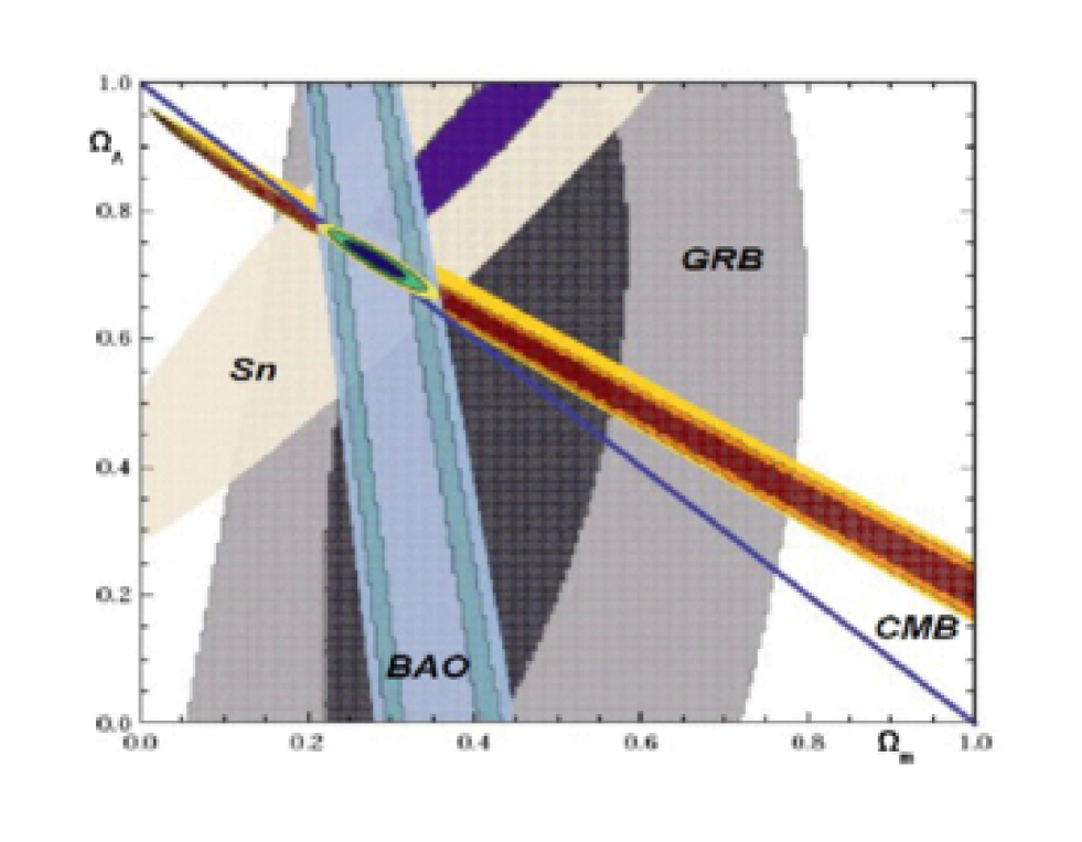
Figure 3: 68%, 95%, and 98% constraints on $\Omega_{\rho}$ and $\Omega_{\Lambda}$ in the $\Lambda$CDM model obtained from CMB (red), BAO (blue), the Union 2 Compilation (gray and blue) and the GRB sample considered in this paper (gray and black). The superimposed contour plot represents the combined final results.

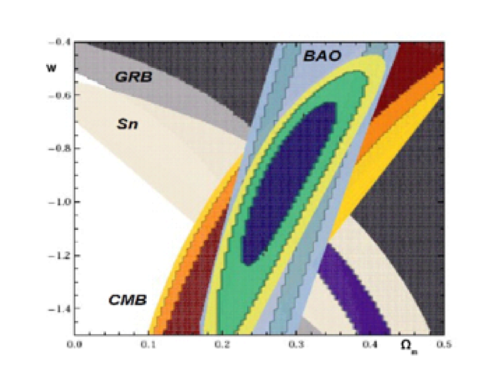
Figure 4: 68%, 95%, and 98% constraints on $\Omega_{\rho}$ and $w$ obtained from CMB (orange), BAO (green), the Union 2 Compilation (gray and blue) and the GRB sample considered in this paper (gray and black). The superimposed contour plot represents the combined final results.

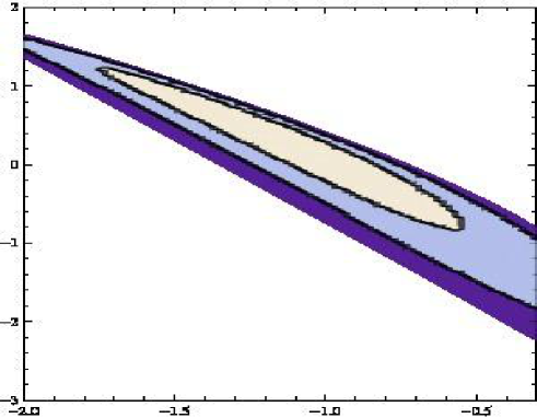
Figure 5: 68%, 95%, and 99.7% constraints on the CPL parameters $w_{0}$ and $w_{a}$ obtained from the Union 2 Compilation and the GRB sample.

Table 2: Final results of our analysis on each cosmological model considered.

Parameter	value	error
$\Lambda$CDM
$\Omega_{m}$	$0.279$	$0.040$
$\Omega_{\Lambda}$	$0.726$	$0.034$
$\Omega_{k}$	$-0.005$	$0.001$
wCDM
$\Omega_{m}$	$0.29$	$0.08$
$w$	$-0.87$	$0.15$
wCDM + CPL
$\Omega_{m}$	$0.27$	$0.08$
$w_{0}$	$-1.18$	$0.38$
$w_{a}$	$0.38$	$0.59$

4 Conclusions

In this work we wondered if the possibility of using GRBs as distance indicators can be a real resource of the modern Precision Cosmology; obviously this deals with the issue that, up to now, we cannot claim that GRBs are standard candles. We developed a statistical (combined) analysis in which the calibration of the luminosity distance has been performed by a SNeIa sample, testing different models ($\Lambda$CDM, $w$CDM and CPL parametrization) with a more complete sample, including GRB data. We obtain satisfactory results especially in the CPL case. We conclude that the present data cannot suggest to us something new about the standard model, but the procedure must be seen as a first application of the use of GRBs in cosmology, for future developments. In a next paper we shall present intriguing results, studying with more accuracy the quoted models and other alternatives.

References

- [Amanullah et al.(2010))] Amanullah R., et al., 2010, arXiv:1004.1711.
- [Amati et al.(2002)] Amati L., et al., 2002, A&A, 390, 81.
- [Amati et al.(2009)] Amati L., et al., 2009, A&A, 508, 173.
- [Butler et al.(2009)] Butler N., et al., ApJ, 2009, 694, 76.
- [Capozziello & Izzo(2010)] Capozziello S. & Izzo L., 2010, A&A, 519, A73.
- [Chevallier & Polarski(2001),Linder(2003)] Chevallier, M., Polarski, D., 2001, Int. J. Mod. Phys. D., 10, 213; Linder, E. V., 2003, Phys. Rev. Lett., 90, 091301.
- [Copeland et al.(2006)] Copeland E.J., Sami M., Tsujikawa S., 2006, Int.J.Mod.Phys.D, 15 1753.
- [Costa et al.(1997)] Costa E., et al., 1997, Nature, 387, 783.
- [D’Agostini(2005)] D’Agostini G., 2005, arXiv:physics/0511182.
- [Eisenstein et al.(2005)] Eisenstein D., et al., 2005, ApJ, 518, 2.
- [Komatsu et al.(2010)] Komatsu E., et al., (2010), arXiv:1001.4538.
- [Liang et al.(2008)] Liang N., et al., (2008), ApJ, 685, 354.
- [Meszaros(2006)] Meszaros P., 2006, Rep. Prog. Phys., 69, 2259.
- [Perlmutter et al.(1999)] Perlmutter, S., et al., (1999), ApJ, 517, 565.
- [Salvaterra et al.(2009)] Salvaterra R., et al., 2009, Nature, 461, 1258.
- [Schaefer(2007)] Schaefer B., 2007, ApJ, 660, 16.
- [Shahmoradi & Nemiroff(2009)] Shahmoradi A. & Nemiroff R.J., 2009, arXiv:0904.1464.
- [Tanvir et al.(2009)] Tanvir N., et al., 2009, Nature, 461, 1254.
- [Visser(2004)] Visser M., 2004, Class. Quant. Grav., 21, 2603.
- [Wang & Mukherjee(2006)] Wang L. & Mukherjee P., 2006, ApJ, 650, 1.
- [Weinberg(1972)] Weinberg, S., 1972, , (Wiley, New York).