CS lines profiles in hot cores

Abstract

We present a theoretical study of CS line profiles in archetypal hot cores. We provide estimates of line fluxes from the CS(1-0) to the CS(15-14) transitions and present the temporal variation of these fluxes. We find that i) the CS(1-0) transition is a better tracer of the Envelope of the hot core whereas the higher-J CS lines trace the ultra-compact core; ii) the peak temperature of the CS transitions is a good indicator of the temperature inside the hot core; iii) in the Envelope, the older the hot core the stronger the self-absorption of CS; iv) the fractional abundance of CS is highest in the innermost parts of the ultra-compact core, confirming the CS molecule as one of the best tracers of very dense gas.

1 Introduction

Understanding how stars form at various redshifts is crucial in order to infer how larger structures such as galaxies are made and evolve in the Universe. To understand the process of star-formation, it is essential to determine the properties of the gas in star-forming regions (hereafter called SFR), both in our own Galaxy and in external galaxies.

SFR encompass a large range of physical and chemical conditions. Within SFR, the gas and dust are recycled from prestellar cores to hot corinos and hot cores. During the star formation cycle, the pressure, density, temperature and chemistry vary.

Numerous papers present atomic and molecular observational surveys of prestellar cores, hot corinos and cores in our own Galaxy (e.g. Ungerechts & Thaddeus 1987; MacDonald et al. 1996; Pratap et al. 1997; Remijan et al. 2003; Kaifu et al. 2004; Ceccarelli 2005; Bottinelli et al. 2007; Olofsson et al. 2007). Determining the gas and dust temperatures, gas density, molecular abundances, etc. of each component in SFR can only be achieved by a close comparison between observations and detailed modelling.

In this paper, we present a theoretical study of the ¹²C³²S (hereafter CS) molecular emission from hot cores, motivated by the work of Doty & Neufeld (1997) and Millar & Hatchell (1998). Subsequent papers will present results for molecules such as methanol, HCO⁺ and HCN. Our first aim is to provide observers with theoretical CS profiles that may help them interpreting the CS line emissions arising from hot cores, such as those from Wu et al. (2010). We do not specifically model any particular hot core. Instead, we model an archetypical hot core composed of ultra-compact core and surrounding envelope. We present estimates of line fluxes and line profiles for comparison with observations.

The study performed by Millar & Hatchell (1998) of the hot cores distinguished two zones of emission: the ultra-compact core (hereafter UCC) and the Envelope of the hot core. While the UCC zone is characterized by a size of about 0.03 pc, an average age of 3.2$\times 10^{3}$ yrs (see Millar & Hatchell 1998) and an average density of 1$\times 10^{7}$ cm^-3, the Envelope corresponds to a more extended region (0.15 pc size) at a lower density (1$\times 10^{6}$cm^-3, see again Millar & Hatchell 1998). In this paper, studies of both the UCC and the Envelope CS line emissions are performed between 1$\times 10^{3}$ yrs and 1$\times 10^{5}$ yrs. It is expected that the Envelope survives longer than the UCC once the protostar(s) is (are) formed. Thus, its emissions should remain detectable at later times than the emissions coming from the UCC. This is why, for the Envelope, we have investigated time up to 1$\times 10^{6}$ yrs.

The key questions we aim to answer in this paper are i) what are the contributions of these two emitting zones to the total CS line emissions detected in hot cores? ii) How do these contributions evolve with the age of the hot core? Answering this question is crucial for improving our current understanding of massive star formation. CS is particularly useful for observers, as it emits quite strongly, not only in hot cores in our own Galaxy (e.g. Beuther et al. 2002; Leurini et al. 2007; Wu et al. 2010) but also in external galaxies (see e.g. Martín et al. 2006; Bayet et al. 2008a; Aladro et al. 2009; Bayet et al. 2009). It is also recognized as to be one of the best tracers of very dense and warm gas with line critical densities of about 10^6-7 cm^-3 (Plume et al., 1992; Linke & Goldsmith, 1980; Snell et al., 1984). In addition, its spectroscopic characteristics are very well known.

In Sect. 2, we describe the models we use and present, for the first time, an interface code we have built between the UCL chemical model (hereafter called UCL_Chem) and the radiative transfer code SMMOL. In Sect. 3, we specify the parameters used for this particular study of the CS molecule emission in hot cores. In Sect. 4 we present our results and we show how the CS line profiles and fluxes vary with evolution of the hot core and different parameters. We discuss the results in Sect. 5 and conclude in Sect. 6.

2 Model descriptions

To generate the CS line profiles, we have developed an intuitive and friendly interface able to couple the UCL_Chem model and the radiative transfer code SMMOL. This Interface code will be very shortly publicly available. The UCL_Chem model is briefly described in Subsect. 2.1 whereas a summary of the main characteristics of SMMOL is presented in Subsect. 2.2. The interface is described in Subsect. 2.3.

2.1 The UCL_Chem model

The UCL_Chem model is fully described in Viti & Williams (1999) and its upgrades are presented in Viti et al. (2004) and Bayet et al. (2008b).

The UCL_Chem is a time-dependent 1-D chemical code that can be used to model the evolution of the gas and dust during the formation of a star. Here we used it to simulate the formation of a hot core. As in Viti et al. (2004), we first model the collapse of a 10K core (Phase I); we then follow the chemical evolution of the remnant core once the star is born (Phase II). The presence of an infrared source in the centre or in the vicinity of the core is simulated by subjecting the core to an increase in the gas and dust temperature.

In both phases, the chemical network is based on more than 1700 chemical reactions taken from the UMIST database (Millar et al., 1997; Le Teuff et al., 2000) involving about 200 species, of which 42 are surface species. The relevant surface reactions included in this model are assumed to be only hydrogenation, allowing chemical saturation where this is possible.

One of the outputs of the UCL_Chem is the fractional abundance (with respect to the total number of hydrogen nuclei) of gas and surface species. See Sect. 3 for a description of the grid of UCL_Chem models ran for this study.

2.2 The SMMOL model

The molecular line radiative transfer code solves the multilevel radiative transfer problem in a 1-d spherical geometry. The code we use, SMMOL, is based upon two codes; Multi-Mol (Yates et al., 1997) and the SMULTI code developed by Harper (1994). SMMOL uses an Accelerated Lambda Iteration (ALI) scheme to speed the convergence of the iterative scheme that is used to solve a set of linearly perturbed kinetic master equations, in order to determine the steady state populations of a molecule’s energy levels and the radiation field. This is the MULTI method described in Scharmer & Carlsson (1985). Subsequently the MALI method (Hummer & Rybicki, 1992) was added to SMMOL; this uses an ALI technique to speed the convergence of a set of preconditioned kinetic master equations.

SMMOL (Spherical Multi-MOL) is a general non-LTE molecular line radiative transfer code that has reproduced the spectral lines observed towards a large number of sources (e.g. Benedettini et al. 2006; Yao et al. 2006; Lerate et al. 2008; Tsamis et al. 2008; Lerate et al. 2010). It is fully described in Rawlings & Yates (2001) and has been benchmarked with other radiative transfer codes in van Zadelhoff et al. (2002). We recommend these papers to any reader. The output line profiles are convolved with user supplied telescope properties using the method described in Schoenberg (1988).

Typically SMMOL uses 400 rays to compute the spherical cloud modelled to compute the intensities at each radial grid-point (hereafter ”shells”) in the cloud. The code is capable of adapting its sampling along each ray to take account of large velocity changes between shells e.g. if the line of sight velocity change between adjacent shells causes the individual line absorption profiles at these adjacent shells to be non overlapping in frequency space; this is not physical and can allow photons to escape the cloud that would otherwise have been absorbed.

2.3 The Interface code

The Interface is a fortran 95 programme, that transforms the output from UCL_Chem into line fluxes and profiles via the use of SMMOL. It is able to model various gas phases from diffuse gas to hot cores. It is currently being developed for AGB stars and planetary nebulae.

The output file of the UCL_Chem model (i.e. fractional abundances as a function of time and depth) is the input file of the Interface. The UCL_Chem provides a grid in optical depth (Av) of fractional abundances of about 200 species, at various time steps. At each time step, the grid in Av has to be adapted to the spatial (linear) grid of shells used later on in SMMOL and described by:

$$r_{i}=\frac{Av\times(1.6\times 10^{21}/met)}{density}-(\Delta r/2.0+(\Delta r\times i))$$ (1)

where $met$ is the metallicity assumed in the UCL_Chem and $\Delta r$ is the thickness of the shells (assumed all equal here - linear distribution of the shells):

$$\Delta r=\frac{size}{n_{shell}}$$ (2)

Then, the Interface also manages the allocation, to each shell of the appropriate physical values, required to run SMMOL. They are the density, temperature, fractional abundance etc which are extracted from UCL_Chem. To do so, the Interface converts Av into distance and interpolate the UCL_Chem values alongside the shell grid using SPLINE and SPLINT functions. For this study, the dust temperature is assumed to be equal to the gas temperature since in the UCL_Chem model, the dust temperature is not calculated. For our models (see Sect. 3), this assumption is valid since the opacity and the density are very high in both the Ultra-compact core and the Envelope (Av $\gg$ 100 mag). Once the Interface has created the correct grid, it automatically runs the SMMOL programme. The outputs of SMMOL are plotted and tabulated by the Interface.

We hope that the Interface will be used to automatically interpret data in from space telescopes (e.g. Herschel, JWST) and observatories (e.g. ALMA, e-Merlin…).

3 Choice of parameters

3.1 General assumptions

The UCL_Chem models are converted into inputs for the SMMOL code using the Interface code, as described in Sect. 2.3. We describe here our choice of parameters and assumptions.

The main sampling parameters such as the number of radial density shells, and the line-of-sight frequency sampling through the cloud, are determined beforehand to ensure that the output fluxes are invariant with respect to sampling for all the models run through SMMOL. We found that $n_{shell}=100$ and 400 lines-of-sight for ray tracing, ensured that the results were invariant; the smallest clouds we sample are actually very oversampled.

We used the first 40 rotational levels of CS in the vibrational ground state; the molecular data and the collisional rates with respect to to H₂ are from the Cologne Database for Molecular Spectroscopy.

The kinetic temperature law (see Eq. 3) we used is a compromise between the need for a power law which is flatter in the inner hot core (to take into account photon trapping effects due to higher optical depths, which slow the cooling of material by radiation) and the need for a 1/r^0.5 law to describe the cooling we would see in the lower optical depth outer cloud. We have used Eq. 3 to be consistent with previous studies (Millar & Hatchell, 1998; Viti & Williams, 1999; Benedettini et al., 2006; Lerate et al., 2008, 2010).

We chose a turbulence velocity of 1.5 kms^-1 (since observations show narrow line profile as in Hatchell et al. 1998b) assumed no velocity gradient, a typical distance of 450pc (Orion-KL: see de Vicente et al. 2002) to the source and solar metallicity. If these hot cores had a large velocity gradient, it would reduce the optical depth of the lines and allow photons to travel more freely in the hot core. The spectra will therefore become less absorbed and line broadening due to optical thickness would be reduced. However the line width would be increased as emission would come from a greater range of velocities. Actually, there is currently little evidence for velocity gradients in these systems. Observations of lines from these systems show narrow lines (e.g. Hatchell et al. 1998b) suggesting that all parts of the UCC and Envelope can be radiatively coupled. The line absorption profile is clearly dominated by turbulence, with the kinetic temperature contributing to the FWHM.

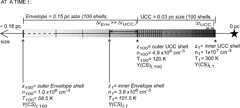
Figure 1: Cartoon representing the structure of the hot core we adopt: the Ultra-compact core UCC (right hand side) and the Envelope (left hand side). The characteristics of each zone, in the multi-points approach, for a certain time t, are specified. The grey scale does not have any physical meaning but should be considered more as an guideline for the eyes. It symbolises the gradient in density and temperature through the hot core with the darkest zones corresponding to the highest values of density and temperature. The shells of width $\Delta r$ are represented by vertical bars from number 1 to 100 (z₁ showing the location of the shell number 1). Regular and italic fonts are used for distinguishing the UCC shells from the shells of the Envelope, respectively.

The cloud was illuminated by the standard interstellar radiation field (Habing, 1968) and the dust extinction model is from Mathis (1990). The emergent spectra were convolved with the appropriate telescope beam (either JCMT or IRAM). To enable us to make useful predictions for ALMA or any interferometric observations (e.g. CARMA, PdBI,…), we need to predict emission from the source at sub-arcsec resolution. The 24 models whose parameters are displayed in Table 1 have been run twice, once with IRAM/JCMT resolutions (line profiles presented as such, see Fig. 2-4), and once with effectively an infinite resolution (radial distribution, see Fig. 5) allowing us thus to get the largest range of (sub-arcsec) resolutions possible. The gas density (see Eq. 4), fractional abundances and cloud size are provided by the UCL_Chem model (see Fig. 1).

Currently the high resolution observational data that exist suggest that objects are ellipsoidal or spherical in shape (Davis et al., 2010; Graves et al., 2010; Wu et al., 2010). We are constrained by the 1-D nature of the UCL_Chem and SMMOL models, which means the only models we can construct are spherical. The most likely effect of non-spherical geometry would be the scenario where collapse was aided by magnetic field lines, giving a flattened density profile with an equatorial enhancement of material. The inclination of the source now becomes important; a pole-on source will have lower optical depth than an equatorial-on source. This means we could, for instance, overestimate the number of low optical systems, and underestimate the mass of objects.

We ran the Interface code for several ages from $1\times 10^{3}$ yrs to $1\times 10^{6}$ yrs (see Table 1). Millar & Hatchell (1998) assumed more specifically a typical age of $3.2\times 10^{3}$ yrs for the Ultra-Compact Core (see Models HC₁, HC₃, HC₅ and HC₇ to HC₁₃) whereas a longer time for a less dense gas such as the one contained in the Envelope (see Models HC₂, HC₄, HC₆ and HC₁₄ to HC₂₄) is expected.

3.2 UCC and Envelope specific assumptions

To reproduce the CS line emission in hot cores for various density and temperature structures and ages, we have run over 80 UCL_Chem models but present here only results from the most interesting ones; the parameter choices made for these 24 calculations are summarized in Table 1.

The size of the region has been set to 0.03 pc for the Ultra-Compact Core and 0.15 pc for the Envelope. Other input parameters such as the FUV radiation field, the cosmic ray ionisation rate, the gas-to-dust mass ratio,… are all set to their standard values as in Bayet et al. (2008b) (see Tables 1, 2 and 3 in their paper).

To represent the UCC zone, we ran the UCL_Chem model with a temperature of 10 K in Phase I, collapsing the core to a critical density of 10⁷cm^-3 (central density: $n_{c}$). We chose a central density of $10^{7}$cm^-3 in order to be consistent with our previous work Bayet et al. (2008b) and because it is the density derived by single-dish observations (Hatchell et al., 1998a). In fact, the central density of hot cores may be higher than that (see interferometric data in Beltrán et al. 2005). However due to the high opacity of hot cores (Av $\gg$100 mags) a small change in the central density should have a negligible effect on the fluxes.

In both regimes (i.e. UCC and Envelope), when no temperature and density profiles are applied (see Models HC₁ and HC₂), the temperature and the density are kept fixed at 300 K and $1.0\times 10^{7}$ cm^-3, respectively, for the UCC zone, and to 101.5 K and $3.8\times 10^{6}$ cm^-3, respectively, for the Envelope case. For Models HC₃ and HC₄, we only applied a density profile (see Sect. 4.1).

When a temperature profile is applied (this was done for Models HC₅ and HC₇ to HC₁₃ using Eq. 3), the temperature varies from 120 K to 300 K (between the lowest to the highest Av, respectively). We used the formula seen in Viti & Williams (1999):

$$T(r)=T_{c}\times(\frac{r}{r_{0}})^{-0.4}$$ (3)

where $T_{c}$=300K is the central temperature typical for hot cores (see Millar & Hatchell 1998; Viti et al. 2004) and $r_{0}$=0.18 pc is the distance from the edge of the hot core to the newly born star (see Fig. 1). When a density profile is applied (e.g. Models HC₃, HC₅ and HC₇ to HC₁₃ and Eq. 4) the density profile, from the lowest to the highest Av, leads to the density varying from $4.9\times 10^{6}$ cm^-3 to $1.0\times 10^{7}$ cm^-3, respectively. We used the same formalism as in Caselli & Myers (1995); Hatchell et al. (2000) and Bacmann et al. (2000), which is effectively a Bonnor-Ebert sphere approximation:

$$n(r)=n_{c}\times(1+\frac{r}{r_{c}})^{-1.5}$$ (4)

where $n_{c}=10^{7}$cm^-3 is the density assumed at the center of the hot core and $r_{c}=0.05$ pc (Nomura & Millar, 2004) is the radius between isothermal and non-thermal velocity effects in hot cores.

To model the Envelope, we have run the UCL_Chem model with a temperature of 10 K in Phase I, letting the UCC collapse to a critical density of $3.8\times 10^{6}$cm^-3 (i.e. the density of the inner shell of the Envelope, see Fig. 1). From the lowest to the highest Av, when a temperature profile is applied (e.g. Models HC₆ and HC₁₄ to HC₂₄ using Eq. 3), the temperature varies from 58.5 K to 101.5 K, respectively. When a density profile is applied (e.g. Models HC₄, HC₆ and HC₁₄ to HC₂₄ using Eq. 4) the density varies from $1.0\times 10^{6}$ cm^-3 to $3.8\times 10^{6}$ cm^-3, respectively.

4 Results

In the following section, we present the results for our study to note the effects of the variations in the internal structure of the hot core (see Subsect. 4.1), and its age (see Subsect. 4.2), and we compare the spectra from the UCC and the Envelope (see Subsect. 4.3), having addressed velocity and geometry effects in Sect. 3.1. Figures 2-4 show examples of the most interesting changes affecting the line profiles whereas Table 1 summarizes for each hot core model the integrated line fluxes of the CS transitions obtained.

4.1 Influence of the density and temperature profiles on the CS line emissions

The influence of the density and temperature profiles on the CS line emissions is shown in Fig.2 (from bottom to top). This figure represents thus results obtained for Models HC₁, HC₃ and HC₅ (for the UCC) and Models HC₂, HC₄ and HC₆ (for the Envelope) whose parameters are seen in Table 1.

In the case of constant density (top plots of Fig. 2), it is interesting to note the differences in the line profile shapes of the low-J CS lines (up to CS(3-2)) as compared to those of the higher-J CS transitions (from CS(4-3)). Firstly, high-J CS lines show the strongest emissions. Secondly, the low-J CS lines have a narrower line width than the high-J CS transitions (by a factor of about $\lesssim$ 1.5-2.0). The first result can be understood by looking at the level population distribution. Indeed, in Model HC₁, the majority of the collisions occur in the high levels of CS, favoring transitions at high-J rather than low-J, whose levels are less populated by one order of magnitude on average. In addition, the transitions between the high-J levels have high $A_{ij}$ coefficients ($A_{ij}$ is proportional to $\nu^{3}$). These factors give also rise to higher source function terms and so to brighter emission. In parallel, the high-J lines, as well as being brighter than low-J transitions, are also broader and show more spectral structure than the low-J transitions. Indeed, the higher-J lines have flatter peaks and some show strong self absorption at the systemic velocity. The line broadening is a consequence of opacity, more often seen in stellar spectra and often called the curve-of-growth. The low optical depth lines have narrow Gaussian line shapes. As the optical depth increases the line centre emission saturates, however the line wing emission can still increase and it is this increase that broadens the line and increases the FWHM of the line. Eventually the line wings saturate and flattened line-shapes are observed. Finally the optical depth at line centre is high enough to promote self absorption and twin-peaked spectra are formed. The observed molecular line curve-of-growth spectral behavior can give a spectral signature for warm dense hot cores.

To disentangle the influence of the density and the temperature profiles on the CS line emissions, we have first kept the temperature constant to 300 K in the UCC and 101.5 K in the Envelope whatever the UCC (Envelope) radial shell (see Models HC₃ and HC₄, respectively). In such case (density profile only), the UCC CS line profile shapes do not seem significantly changed as compared to the case where there is no profile. On the contrary, for the Envelope, where the difference in densities between the outer and the inner shells is steeper than for the UCC, we see more significant changes.

However, one notes that for Model HC₃, a slight broadening of all the lines is seen, between a factor of 0.33 and 0.16 for the CS(1-0) and the CS(7-6) transitions, respectively. In addition, the peak antennae temperatures are on average weaker than in the case where no profile is applied (differences varying between 3 K and 12 K). A saturation in the CS(7-6) profile is also seen. This is due to the higher fractional abundances of CS obtained from the chemical model (see Table 1).

Finally when we add the temperature structure (see Model HC₅ for the UCC and Model HC₆ for the Envelope), we see that (Fig. 2), the peak antennae temperatures of all the CS lines but CS(1-0) in the Envelope are indeed weaker by a factor of 1.5. To be more precise, we found that the modelled Tpeaks change in all 80 models when we implement a $r^{-0.4}$ temperature profile as compared to their values without. It means that the distribution of the temperatures inside the hot core, i.e. the temperature variation seen from shell to shell, do have a consequence for the integrated (”total”) profiles of CS lines. The differences in the Tpeak values range from 20% to a factor of two, depending on the line and the source considered (see in Fig. 2 the bottom two plots for UCC and Envelope: both show a decrease of the CS line Tpeak when a temperature profile is implemented). We believe that ALMA may be sensitive to factors as small as this in Tpeak. In fact already with the CARMA and IRAM-Plateau de Bure Interferometer such factors are detectable for hot cores (Wu et al., 2010). It may therefore be possible to estimate Tc and potentially reconstruct the temperature profile of the observed source by using Eq. 3.

All the lines (except J=1-0) are thus good probes of these changes in temperature. The peak antennae temperature is a measure of the gas kinetic temperature if the gas is in LTE, the column is optically thick and the source is resolved by the telescope at the observing frequency.

The CS(1-0) does not seem affected at early times by the changes in temperature in the Envelope. This might come from the fact that the fractional abundance of CS is quite low in the Envelope. The $A_{ij}$ is also 300 times less for the J=1-0 transition compared to the J=7-6 transition. Also the energy of the J=1 level $E_{(J=1)}=2.35$ K, which means that in a gas of 50-100 K its population is comparatively less than in clouds where T=10 K. This is why the 1-0 line is the weakest line in both the Envelope and the UCC. However the fractional abundance of CS increases by 20 in the Envelope during its evolution and that is why the line strength grows and the line starts to become flat topped.

4.2 Influence of the age of the hot core on the CS line emissions

Figure 3 shows the evolution of UCC CS lineshapes with the evolution of the hot core. We see the high-J lines increase in flux with time and become increasingly flattened, broader and self absorbed; some eventually produce twin peaked spectra. The low-J lines grow to large intensities with time and also show flattened profiles at large times.

Figure 4 shows the evolution of Envelope CS lineshapes with the evolution of the hot core. It shows that transitions for J=5, 4, 3, 2 are initially the brightest transitions, with the J=2-1 transition being the brightest line; the J=3 to 7 transitions are self absorbed at all times, with the J=7-6 line being the broadest line. The J=1-0 transition is initially the least bright and narrowest line.

By the largest time, the J=7 to 2 transitions are now all self absorbed and have basically the same width. There has been a modest increase in the peak flux of these lines. The J=1-0 line is now very bright, broader and has a flat top.

The UCC lines are brighter than the Envelope lines. For the Envelope, the best tracer of age seems to be the CS(1-0) transition which shows the largest variations in fluxes with respect to time (see Models HC₁₄ to HC₂₄). In principle, this transition could be used as an evolutionary indicator. However we note that the sulphur-bearing chemistry depends very critically on the gas temperature and density (as also found by Wakelam et al. 2004; Viti et al. 2004) and hence, care must be taken to constrain initial conditions. In the case of the UCC, the differences in fluxes from $1\times 10^{3}$ yrs to $1\times 10^{6}$ yrs may not be large enough to be detectable.

4.3 Influence of the size of the hot core on the CS line emissions

There are, as expected, clear differences between UCC CS line emissions and those coming from the Envelope (see Figs. 2, 3 and 4 and Table 1). We restrict our comparison to the most realistic cases which are the cases where both density and temperature profiles are applied to the two zones.

A first interesting remark concerns the radial distribution of the CS fractional abundance, for a given time. From column 9 of Table 1, for a fixed time (e.g. $3.2\times 10^{3}$ yrs ) one notes that, from the inner UCC shell (closest to the star) to the outer Envelope shell (edge of the hot core), the CS fractional abundances does not increase nor decrease constantly (see paired models in Table 1). In fact, Table 1 shows that the CS fractional abundance is predominantly produced in the UCC inner zone of the hot core, confirming CS as preferentially linked with very dense gas, and therefore could be considered as an ideal tracer of this gas phase (see also Linke & Goldsmith 1980; Snell et al. 1984). For example, we can see that for the coupled models HC₃ and HC₄, the UCC (HC₃) abundance of CS is $1.72\times 10^{-8}$ whereas the Envelope (HC₄) can account for only $3.77\times 10^{-9}$. This is a factor of 4.6 difference. In other words, the UCC produces 4.6 times more CS (in abundance) than the Envelope. For other models, the difference are of 2.6 (HC₈ and HC₁₅), 7.2 (HC₉ and HC₁₆), 9.6 (HC₁₀ and HC₁₇), 12.1 HC₁₁ and HC₁₈), 17.6 (HC₁₂ and HC₂₀) and 11.5 (HC₁₃ and HC₂₂). The only models where the CS is not predominantly produced by the UCC is the pair HC₇ and HC₁₄ (difference of 0.9 only).

The radial integrated CS line fluxes distribution is shown in Fig. 5 at $3.2\times 10^{3}$ yrs (as assumed in Millar & Hatchell 1998). We note that the line flux distribution as a function of radius at different times (not shown) are the same as those shown in Fig. 5. Note that, for the plots shown in Fig. 5, we did not apply any telescope convolution when we have run SMMOL because we wanted to identify all the emission from the UCC and the Envelope (hence the differences in CS line fluxes between Table 1 and Fig. 5). For both plots in Fig. 5, the protostar is located at the origin of the x-axis (right hand side) following the convention adopted in Fig 1. The maxima integrated CS line fluxes are located on the plots by a thick black cross. The maxima are all distributed in the UCC within a restricted radius ($8-9\times 10^{16}$ cm from the source) whereas for the Envelope, their position is more spread ($3.5-5.5\times 10^{17}$ cm from the source). In the Envelope, the CS lines fluxes maxima, from 1-0 to 10-9 are distributed deeper and deeper inside the gas. A turnover occurs for the maximum of the CS(10-9) line flux. From this transition onwards up to the CS(15-14) line, the maxima location is moving towards the edge of the Envelope. The turnover is actually controlled by the competition between the source function and absorption terms at each radius. These terms depend upon volume of gas at a radius, the population of the levels and the Einstein $A$ coefficients of the transitions (Note that $A_{ij}$ increases with J). In the Envelope this produces most flux for the J=10-9 transition. The turnover at large radii is caused by the reduction in the source function and optical depth due to decrease of gas density and temperature.

In the UCC, the same factors affect the line emission as for the Envelope. The higher density and temperature explain why the J=13-12 emission is the brightest transition. The turnover happens proportionately much closer to the UCC outer edge than in the Envelope and thus does not appear clearly. This is because the optical depth and source functions of the optically thick lines drops due to falling densities and temperatures and these actually cause the low J lines to turnover as well.

Here, we have simplistically assumed that when a hot core is observed the total CS flux (taking into account the self-absorption) is, to a first order approximation, equal to the sum of the emission coming from the UCC and from the Envelope. Millar & Hatchell (1998) in their study, assume that hot cores can be as large as 1 pc size and consequently that there is a potential third contribution to the total molecular emission from the halo (see Millar & Hatchell 1998). We did not investigate such region in this paper since the halo is much more diffuse than the Envelope and the UCC, and the CS may not be a good tracer of such gas.

As seen from Fig. 5, contrarily to the CS(1-0), (2-1) and (3-2) line fluxes, it is interesting to note that the high-J CS line fluxes (from 6-5) are mainly emitted from the UCC zone (factors of differences between the Envelope and the UCC contributions from 3.6 to 13.1 - see also Table 1). This makes the low-J and the high-J CS lines better tracers of the Envelope and the UCC, respectively. This result can only be confirmed by interferometric observations. The envelope has a lower hydrogen number density and kinetic temperature, i.e. $E_{(J=7)}=49.3$ K than the UCC. The CS rotational high-J levels in the UCC are therefore more highly populated that the same levels in the envelope. Although the UCC is smaller than the Envelope the excited column at high-J levels in the UCC is brighter than that in the Envelope. In the UCC (T=100-300K) the J=1 level is very underpopulated as compared to the Envelope and therefore has a much lower optical depth and source function; it is for this reason that despite the fractional abundance of CS increasing we see a weak J=1-0 line at all times in the UCC.

Finally we note that in the case of the Envelope, the lines between J=2-1 and J=6-5 show similar widths (within a factor of 1-2 kms^-1), contrarily to the UCC case where line widths are quite different from a transition to another. The high-J lines remain optically thin for much longer in the UCC than for the Envelope. The absorption profile of each line is slightly broader because of the higher kinetic temperature in the UCC (0.2-0.3 kms^-1)

5 Discussion

Unfortunately, there are no complete (i.e. from J=2-1 to J=7-6) datasets of interferometric CS observations for hot cores. CS data presented in Hauschildt et al. (1995); MacDonald et al. (1996); Beuther et al. (2002); Beltrán et al. (2005) and Leurini et al. (2007) focuss only on certain transitions of CS or on isotopologues of CS. On the other hand, multiples lines of ¹²C³²S are observed in galactic hot cores but only using single-dish instruments. Despite these limitations, qualitative comparison of our results with the data presented in Murata et al. (1994); Chandler & Wood (1997) and more recently in Wu et al. (2010) can be made. Of particular interest, Wu et al. (2010) found that the CS(2-1) transition is indeed less compact than the CS(7-6) as seen in maps of 50 massive very dense galactic sources. This agrees very well with our model predictions and seems to confirm that the high-J CS lines are one of the best tracers of very dense compact gas (i.e. better than HCN). Similarly, they found that their mean and median linewidth increase for high-J CS lines, which is also in agreement with our model predictions. Here we do not attempt to model any of the sources of their sample but the fact that our theoretical approach and their observational results converge is encouraging.

Fig. 5 thus used by observers to estimate integration times as it gives the expected flux of the first 15 transitions of CS at various resolution (i.e. various radii). The fluxes are generally produced by a combination of a chemical model, line and continuum radiative transfer code and telescope convolution algorithm. The deconvolved fluxes presented in Fig. 5 can be used to estimate fluxes for other telescope parameters and source distances. For different source types and masses, an observer can scale these results, but the scaled results would be approximate at best. With interferometers such as the IRAM-Plateau de Bure, spatial resolutions up to $7\times 10^{16}$ cm are already accessible (for a distance of 450 pc). As an example, de Vicente et al. (2002) already performed a detailed study of HC₃N in the Orion KL hot core. With Fig. 5, we show that similar studies are possible for CS. Indeed, a resolution of 5 ^′′ is reached in de Vicente et al. (2002) work, which corresponds to 0.01 pc (i.e. 3.856$\times 10^{16}$ cm) i.e. the CS UCC zone emission. More information on the structure of the CS emission in hot cores will be obtainable soon with ALMA.

6 Conclusions

We have performed a systematic theoretical study of the line intensities and the properties of CS in archetypical hot core environments. We have coupled via a user-friendly interface, a large grid of chemical models with SMMOL radiative transfer code and obtained line profiles of the CS(1-0) to CS(15-14) lines for a variety of density, temperature, size and age. We also provide (Fig. 5) observers with estimates of line fluxes at various resolution for the first 15 transitions of CS molecule.

Our main conclusions are:

• the CS fractional abundance is highest in the innermost parts of the UCC whatever the age of the hot core. This confirms the CS molecule as one of the best tracers of the very dense gas component (see Sect. 4.3).
  

• the high-J CS lines have the strongest line fluxes, and the linewidths are broader than those of low-J CS lines (see Sect. 4.1).
  

• The peak antennae temperature of all the CS transitions except for the CS(1-0) line is a good tracer of the kinetic temperature inside the hot core because it is very sensitive to its changes (see Sect. 4.1).
  

• In the Envelope, the older the hot core, the stronger the self-absorption of CS. The best tracer of age seems to be the CS(1-0) line which show the largest variations in fluxes with respect to the time (see Sect. 4.2).
  

• The CS(1-0) flux is coming mainly from the Envelope while the high-J CS line fluxes are better tracers of the UCC zone (see Sect. 4.3).
  

Figure 2: Variation of the CS line profiles for the UCC (left, from top to bottom: Models HC₁, HC₃ and HC₅) and the Envelope (right, from top to bottom: Models HC₂, HC₄ and HC₆) when various internal hot core structures are used. From top to bottom, we have applied no profiles, only a profile in density, and a profile in both density and temperatures (see Sect.3 and Subsect.4.1). The CS line profiles are expressed in antennae temperature (in K) using the IRAM and the JCMT resolutions for low-J and high-J CS lines, respectively.

Figure 3: Variation of the CS line profiles for the UCC with time (age plotted in the third dimension: Models HC₇, HC₈, HC₅, HC₉, HC₁₀, HC₁₂ and HC₁₃, respectively).

Figure 4: Variation of the CS line profiles for the Envelope with time (age plotted in the third dimension: Models HC₁₄, HC₁₅, HC₆, HC₁₆, HC₁₇, HC₂₀, HC₂₂ and HC₂₄, respectively). Since it is expected that the Envelope survives longer than the UCC zone, our study has been extended up to $1\times 10^{6}$ yrs.

Figure 5: Variation of the CS integrated line fluxes for the UCC (right hand side) and the Envelope (left hand side). See text in Subsect. 4.3

Table 1: Summary of model runs. “-” means no density or temperature profiles whereas “+” means a profile has been applied. The CS line fluxes are displayed in units of $10^{-15}$ Wm^-2. For each line, we specify the corresponding frequency in GHz. We have giving examples of paired models (see brackets in columns 1 and 2) representing the coupling of the UCC with the Envelope for a particular age. In column 9 we have listed only the values of the CS abundance found at the outer and inner shells for each model. The evolution of the CS abundance alongside the core can thus be studied by looking continously at the columns 9 of the models belonging to the same pair.

		Model	Type	size	density	temperature	age	Frac. abund. of	CS(1-0)	CS(3-2)	CS(7-6)	CS(10-9)
		name		(pc)	profile	profile	(yrs)	CS (outer-inner shell)	48.99 GHz	146.97 GHz	342.88 GHz	489.75 GHz
{		HC1	UCC	0.03	-	-	$3.2\times 10^{3}$	$7.66\times 10^{-9}$	$1.14\times 10^{-4}$	$1.85\times 10^{-2}$	$2.38\times 10^{-1}$	$3.90\times 10^{-1}$
		HC2	Env.	0.15	-	-	$3.2\times 10^{3}$	$1.97\times 10^{-9}$	$3.02\times 10^{-3}$	$4.03\times 10^{-2}$	$1.07\times 10^{-1}$	$1.31\times 10^{-1}$
{		HC3	UCC	0.03	+	-	$3.2\times 10^{3}$	$1.44-1.72\times 10^{-8}$	$1.32\times 10^{-4}$	$2.13\times 10^{-2}$	$2.35\times 10^{-1}$	$3.67\times 10^{-1}$
		HC4	Env.	0.15	+	-	$3.2\times 10^{3}$	$3.77-2.34\times 10^{-9}$	$2.37\times 10^{-3}$	$3.40\times 10^{-2}$	$7.40\times 10^{-2}$	$7.38\times 10^{-2}$
{		HC5	UCC	0.03	+	+	$3.2\times 10^{3}$	$0.55-2.0\times 10^{-8}$	$5.92\times 10^{-5}$	$9.81\times 10^{-3}$	$1.21\times 10^{-1}$	$1.90\times 10^{-1}$
		HC6	Env.	0.15	+	+	$3.2\times 10^{3}$	$4.33-2.37\times 10^{-9}$	$3.10\times 10^{-3}$	$2.89\times 10^{-2}$	$5.70\times 10^{-2}$	$5.90\times 10^{-2}$
—		HC7	UCC	0.03	+	+	$1.0\times 10^{3}$	$2.58-3.28\times 10^{-9}$	$2.36\times 10^{-5}$	$4.39\times 10^{-3}$	$6.97\times 10^{-2}$	$1.04\times 10^{-1}$
$\mid$	—	HC8	UCC	0.03	+	+	$2.0\times 10^{3}$	$3.76-9.82\times 10^{-9}$	$3.56\times 10^{-5}$	$6.39\times 10^{-3}$	$9.22\times 10^{-2}$	$1.42\times 10^{-1}$
$\mid$	$\mid$	HC9	UCC	0.03	+	+	$5.0\times 10^{3}$	$0.82-3.71\times 10^{-8}$	$1.10\times 10^{-4}$	$1.52\times 10^{-2}$	$1.53\times 10^{-1}$	$2.42\times 10^{-1}$
$\mid$	$\mid$	HC10	UCC	0.03	+	+	$7.0\times 10^{3}$	$1.16-5.89\times 10^{-8}$	$1.73\times 10^{-4}$	$1.96\times 10^{-2}$	$1.73\times 10^{-1}$	$2.74\times 10^{-1}$
$\mid$	$\mid$	HC11	UCC	0.03	+	+	$1.0\times 10^{4}$	$1.64-9.33\times 10^{-8}$	$2.61\times 10^{-4}$	$2.35\times 10^{-2}$	$1.88\times 10^{-1}$	$3.00\times 10^{-1}$
$\mid$	$\mid$	HC12	UCC	0.03	+	+	$5.0\times 10^{4}$	$0.55-4.92\times 10^{-7}$	$7.59\times 10^{-4}$	$3.28\times 10^{-2}$	$2.29\times 10^{-1}$	$3.64\times 10^{-1}$
$\mid$	$\mid$	HC13	UCC	0.03	+	+	$1.0\times 10^{5}$	$8.89-4.79\times 10^{-7}$	$9.37\times 10^{-4}$	$3.48\times 10^{-2}$	$2.39\times 10^{-1}$	$3.74\times 10^{-1}$
$\mid$	$\mid$	HC14	Env.	0.15	+	+	$1.0\times 10^{3}$	$3.42-2.62\times 10^{-9}$	$2.66\times 10^{-3}$	$2.79\times 10^{-2}$	$5.52\times 10^{-2}$	$5.60\times 10^{-2}$
—	$\mid$	HC15	Env.	0.15	+	+	$2.0\times 10^{3}$	$3.81-2.44\times 10^{-9}$	$2.86\times 10^{-3}$	$2.83\times 10^{-2}$	$5.59\times 10^{-2}$	$5.72\times 10^{-2}$
	—	HC16	Env.	0.15	+	+	$5.0\times 10^{3}$	$5.15-2.50\times 10^{-9}$	$3.47\times 10^{-3}$	$2.97\times 10^{-2}$	$5.86\times 10^{-2}$	$6.17\times 10^{-2}$
		HC17	Env.	0.15	+	+	$7.0\times 10^{3}$	$6.16-2.83\times 10^{-9}$	$3.87\times 10^{-3}$	$3.06\times 10^{-2}$	$6.04\times 10^{-2}$	$6.47\times 10^{-2}$
		HC18	Env.	0.15	+	+	$1.0\times 10^{4}$	$7.74-3.51\times 10^{-9}$	$4.42\times 10^{-3}$	$3.17\times 10^{-2}$	$6.28\times 10^{-2}$	$6.85\times 10^{-2}$
		HC19	Env.	0.15	+	+	$2.0\times 10^{4}$	$13.77-7.29\times 10^{-9}$	$5.83\times 10^{-3}$	$3.45\times 10^{-2}$	$6.88\times 10^{-2}$	$7.73\times 10^{-2}$
		HC20	Env.	0.15	+	+	$5.0\times 10^{4}$	$2.79-2.06\times 10^{-8}$	$7.45\times 10^{-3}$	$3.82\times 10^{-2}$	$7.70\times 10^{-2}$	$8.78\times 10^{-2}$
		HC21	Env.	0.15	+	+	$7.0\times 10^{4}$	$3.45-2.58\times 10^{-8}$	$7.90\times 10^{-3}$	$3.92\times 10^{-2}$	$7.94\times 10^{-2}$	$9.05\times 10^{-2}$
		HC22	Env.	0.15	+	+	$1.0\times 10^{5}$	$4.17-3.21\times 10^{-8}$	$8.27\times 10^{-3}$	$4.03\times 10^{-2}$	$8.18\times 10^{-2}$	$9.31\times 10^{-2}$
		HC23	Env.	0.15	+	+	$5.0\times 10^{5}$	$9.53-7.29\times 10^{-8}$	$9.79\times 10^{-3}$	$4.58\times 10^{-2}$	$9.43\times 10^{-2}$	$1.06\times 10^{-1}$
		HC24	Env.	0.15	+	+	$1.0\times 10^{6}$	$11.89-1.33\times 10^{-8}$	$1.00\times 10^{-2}$	$4.61\times 10^{-2}$	$9.48\times 10^{-2}$	$1.05\times 10^{-1}$

References

- Aladro et al. (2009) Aladro, R., Martin, S., Martin-Pintado, J., & Bayet, E. 2009, ApJ, in preparation
- Bacmann et al. (2000) Bacmann, A., André, P., Puget, J., Abergel, A., Bontemps, S., & Ward-Thompson, D. 2000, A&A, 361, 555
- Bayet et al. (2009) Bayet, E., Aladro, R., Martín, S., Viti, S., & Martín-Pintado, J. 2009, ApJ, 707, 126
- Bayet et al. (2008a) Bayet, E., Lintott, C., Viti, S., Martín-Pintado, J., Martín, S., Williams, D. A., & Rawlings, J. M. C. 2008a, ApJ, 685, L35
- Bayet et al. (2008b) Bayet, E., Viti, S., Williams, D. A., & Rawlings, J. M. C. 2008b, ApJ, 676, 978
- Beltrán et al. (2005) Beltrán, M. T., Cesaroni, R., Neri, R., Codella, C., Furuya, R. S., Testi, L., & Olmi, L. 2005, A&A, 435, 901
- Benedettini et al. (2006) Benedettini, M., Yates, J. A., Viti, S., & Codella, C. 2006, MNRAS, 370, 229
- Beuther et al. (2002) Beuther, H., Schilke, P., Menten, K. M., Motte, F., Sridharan, T. K., & Wyrowski, F. 2002, ApJ, 566, 945
- Bottinelli et al. (2007) Bottinelli, S., Ceccarelli, C., Williams, J. P., & Lefloch, B. 2007, A&A, 463, 601
- Caselli & Myers (1995) Caselli, P. & Myers, P. C. 1995, ApJ, 446, 665
- Ceccarelli (2005) Ceccarelli, C. 2005, in IAU Symposium, Vol. 231, Astrochemistry: Recent Successes and Current Challenges, ed. D. C. Lis, G. A. Blake, & E. Herbst, 1–16
- Chandler & Wood (1997) Chandler, C. J. & Wood, D. O. S. 1997, MNRAS, 287, 445
- Davis et al. (2010) Davis, C. J., Chrysostomou, A., Hatchell, J., Wouterloot, J. G. A., Buckle, J. V., Nutter, D., Fich, M., Brunt, C., Butner, H., & Cavanagh, B. 2010, MNRAS, 405, 759
- de Vicente et al. (2002) de Vicente, P., Martín-Pintado, J., Neri, R., & Rodríguez-Franco, A. 2002, ApJ, 574, L163
- Doty & Neufeld (1997) Doty, S. D. & Neufeld, D. A. 1997, ApJ, 489, 122
- Graves et al. (2010) Graves, S. F., Richer, J. S., Buckle, J. V., Duarte-Cabral, A., Fuller, G. A., & Hogerheijde, M. R. 2010, ArXiv e-prints
- Habing (1968) Habing, H. J. 1968, Bull. Astron. Inst. Netherlands, 19, 421
- Harper (1994) Harper, G. M. 1994, MNRAS, 268, 894
- Hatchell et al. (2000) Hatchell, J., Fuller, G. A., Millar, T. J., Thompson, M. A., & Macdonald, G. H. 2000, A&A, 357, 637
- Hatchell et al. (1998a) Hatchell, J., Thompson, M. A., Millar, T. J., & MacDonald, G. H. 1998a, A&AS, 133, 29
- Hatchell et al. (1998b) —. 1998b, A&A, 338, 713
- Hauschildt et al. (1995) Hauschildt, H., Güsten, R., & Schilke, P. 1995, in Lecture Notes in Physics, Berlin Springer Verlag, Vol. 459, The Physics and Chemistry of Interstellar Molecular Clouds, ed. G. Winnewisser & G. C. Pelz, 52–53
- Hummer & Rybicki (1992) Hummer, D. G. & Rybicki, G. B. 1992, ApJ, 387, 248
- Kaifu et al. (2004) Kaifu, N., Ohishi, M., Kawaguchi, K., Saito, S., Yamamoto, S., Miyaji, T., Miyazawa, K., Ishikawa, S., Noumaru, C., Harasawa, S., Okuda, M., & Suzuki, H. 2004, PASJ, 56, 69
- Le Teuff et al. (2000) Le Teuff, Y. H., Millar, T. J., & Markwick, A. J. 2000, A&AS, 146, 157
- Lerate et al. (2008) Lerate, M. R., Yates, J., Viti, S., Barlow, M. J., Swinyard, B. M., White, G. J., Cernicharo, J., & Goicoechea, J. R. 2008, MNRAS, 387, 1660
- Lerate et al. (2010) Lerate, M. R., Yates, J. A., Barlow, M. J., Viti, S., & Swinyard, B. M. 2010, ArXiv e-prints
- Leurini et al. (2007) Leurini, S., Beuther, H., Schilke, P., Wyrowski, F., Zhang, Q., & Menten, K. M. 2007, A&A, 475, 925
- Linke & Goldsmith (1980) Linke, R. A. & Goldsmith, P. F. 1980, ApJ, 235, 437
- MacDonald et al. (1996) MacDonald, G. H., Gibb, A. G., Habing, R. J., & Millar, T. J. 1996, A&AS, 119, 333
- Martín et al. (2006) Martín, S., Mauersberger, R., Martín-Pintado, J., Henkel, C., & García-Burillo, S. 2006, ApJS, 164, 450
- Mathis (1990) Mathis, J. S. 1990, ARA&A, 28, 37
- Millar & Hatchell (1998) Millar, T. J. & Hatchell, J. 1998, in Chemistry and Physics of Molecules and Grains in Space. Faraday Discussions No. 109, 15
- Millar et al. (1997) Millar, T. J., MacDonald, G. H., & Gibb, A. G. 1997, A&A, 325, 1163
- Murata et al. (1994) Murata, Y., Kawabe, R., Ishiguro, M., Morita, K., Hasegawa, T., & Hayashi, M. 1994, in Astronomical Society of the Pacific Conference Series, Vol. 59, IAU Colloq. 140: Astronomy with Millimeter and Submillimeter Wave Interferometry, ed. M. Ishiguro & J. Welch, 236–+
- Nomura & Millar (2004) Nomura, H. & Millar, T. J. 2004, A&A, 414, 409
- Olofsson et al. (2007) Olofsson, A. O. H., Persson, C. M., Koning, N., Bergman, P., Bernath, P. F., Black, J. H., Frisk, U., Geppert, W., Hasegawa, T. I., Hjalmarson, Å., Kwok, S., Larsson, B., Lecacheux, A., Nummelin, A., Olberg, M., Sandqvist, A., & Wirström, E. S. 2007, A&A, 476, 791
- Plume et al. (1992) Plume, R., Jaffe, D. T., & Evans, II, N. J. 1992, ApJS, 78, 505
- Pratap et al. (1997) Pratap, P., Bergin, E. A., Dickens, J., Irvine, W. M., Miralles, M. P., Schloerb, F. P., & Snell, R. 1997, in IAU Symposium, Vol. 170, IAU Symposium, ed. W. B. Latter, S. J. E. Radford, P. R. Jewell, J. G. Mangum, & J. Bally, 447–+
- Rawlings & Yates (2001) Rawlings, J. M. C. & Yates, J. A. 2001, MNRAS, 326, 1423
- Remijan et al. (2003) Remijan, A., Snyder, L. E., Friedel, D. N., Liu, S., & Shah, R. Y. 2003, ApJ, 590, 314
- Scharmer & Carlsson (1985) Scharmer, G. B. & Carlsson, M. 1985, Journal of Computational Physics, 59, 56
- Schoenberg (1988) Schoenberg, K. 1988, A&A, 195, 198
- Snell et al. (1984) Snell, R. L., Goldsmith, P. F., Erickson, N. R., Mundy, L. G., & Evans, II, N. J. 1984, ApJ, 276, 625
- Tsamis et al. (2008) Tsamis, Y. G., Rawlings, J. M. C., Yates, J. A., & Viti, S. 2008, MNRAS, 388, 898
- Ungerechts & Thaddeus (1987) Ungerechts, H. & Thaddeus, P. 1987, ApJS, 63, 645
- van Zadelhoff et al. (2002) van Zadelhoff, G., Dullemond, C. P., van der Tak, F. F. S., Yates, J. A., Doty, S. D., Ossenkopf, V., Hogerheijde, M. R., Juvela, M., Wiesemeyer, H., & Schöier, F. L. 2002, A&A, 395, 373
- Viti et al. (2004) Viti, S., Collings, M. P., Dever, J. W., McCoustra, M. R. S., & Williams, D. A. 2004, MNRAS, 354, 1141
- Viti & Williams (1999) Viti, S. & Williams, D. A. 1999, MNRAS, 305, 755
- Wakelam et al. (2004) Wakelam, V., Caselli, P., Ceccarelli, C., Herbst, E., & Castets, A. 2004, A&A, 422, 159
- Wu et al. (2010) Wu, J., Evans, N., Shirley, Y., & Knez, C. 2010, ArXiv e-prints
- Yao et al. (2006) Yao, L., Bell, T. A., Viti, S., Yates, J. A., & Seaquist, E. R. 2006, ApJ, 636, 881
- Yates et al. (1997) Yates, J. A., Field, D., & Gray, M. D. 1997, MNRAS, 285, 303