EFFECTS OF TURBULENCE, ECCENTRICITY DAMPING, AND MIGRATION RATE ON THE CAPTURE OF PLANETS INTO MEAN MOTION RESONANCE

Abstract

Pairs of migrating extrasolar planets often lock into mean motion resonance as they drift inward. This paper studies the convergent migration of giant planets (driven by a circumstellar disk) and determines the probability that they are captured into mean motion resonance. The probability that such planets enter resonance depends on the type of resonance, the migration rate, the eccentricity damping rate, and the amplitude of the turbulent fluctuations. This problem is studied both through direct integrations of the full 3-body problem, and via semi-analytic model equations. In general, the probability of resonance decreases with increasing migration rate, and with increasing levels of turbulence, but increases with eccentricity damping. Previous work has shown that the distributions of orbital elements (eccentricity and semimajor axis) for observed extrasolar planets can be reproduced by migration models with multiple planets. However, these results depend on resonance locking, and this study shows that entry into – and maintenance of – mean motion resonance depends sensitively on migration rate, eccentricity damping, and turbulence.

1 INTRODUCTION

The past decade has led to tremendous progress in our understanding of extrasolar planets and the processes involved in planet formation. These advances involve both observations, which now include the detection of hundreds of planets outside our Solar System (see, e.g., Udry et al. 2007 for a recent review), along with a great deal of accompanying theoretical work. One surprising result from the observations is the finding that extrasolar planets display a much wider range of orbital configurations than was originally anticipated. Planets thus move (usually inward) from their birth sites, while they are forming or immediately thereafter, in a process known as planet migration (e.g., see Papaloizou & Terquem 2006 and Papaloizou et al. 2007 for recent reviews).

Many of the observed solar systems contain multiple planets, and many others may be found in the near future. For systems that contain more than one planet, theoretical work indicates that the migration process often results in planets entering into mean motion resonance (e.g., Lee & Peale 2002, Nelson & Papaloizou 2002), at least for some portion of their migratory phase of evolution. During this epoch, interacting planets (which are often in or near resonance) tend to excite the orbital eccentricity of both bodies. This planet scattering process, acting in conjunction with inward migration due to torques from circumstellar disks, can produce broad distributions of both semi-major axis and eccentricity (Adams & Laughlin 2003, Moorhead & Adams 2005, Chatterjee et al. 2008, Ford & Rasio 2008); these distributions of orbital elements are comparable to those of the current observational sample, although significant uncertainties remain. In any case, the final orbital elements at the end of the migration epoch — and planetary survival — depend sensitively on whether or not the planets enter into mean motion resonance.

These systems are highly chaotic, and display extreme sensitivity to initial conditions, so that the outcomes must be described statistically. Nonetheless, the distributions of final system properties are well-defined and depend on whether the planets enter into mean motion resonance as they migrate inwards; the outcomes also depend on the type of resonance and how deeply the planets are bound into a resonant state. The circumstellar disks that drive inward migration also produce damping and/or excitation (Goldreich & Sari 2003, Ogilvie & Lubow 2003) of orbital eccentricity, and this complication affects the maintenance of resonance. The disks are also expected to be turbulent, through the magneto-rotational instability (MRI) and/or other processes (Balbus & Hawley 1991). With sufficient amplitude and duty cycle, this turbulence also affects the maintenance of mean motion resonance (Adams et al. 2008, Lecoanet et al. 2009, Rein & Papaloizou 2009), and thereby affects the distributions of orbital elements resulting from migration (Moorhead 2008).

The goal of this paper is to understand the probability for migrating planets to enter into mean motion resonance and the probability for survival of the resulting resonant states. Previous work has shown that entry into resonance is affected by the migration rate (Quillen 2006), where fast migration acts to compromise resonant states. This study expands upon previous efforts by considering the effects of not only the migration rate, but also eccentricity damping and turbulent forcing on the probability of attaining and maintaining a resonant state. This paper considers the action of these three variables, jointly and in isolation, and covers a wide range of parameter space. In addition, we address the problem through both numerical and semi-analytic approaches (where ‘semi-analytic’ refers to models where the equations are reduced to, at most, ordinary differential equations.) The results depend on the type of resonance under consideration; this work considers a range of cases, but focuses on the 2:1, 5:3, and 3:2 mean motion resonances.

This paper is organized as follows. We first perform a large ensemble of numerical integrations in Section 2. These numerical experiments follow two planets undergoing convergent migration, and include both eccentricity damping and forcing terms due to turbulent fluctuations. The results provide an estimate for the survival of systems in resonance as a function of migration rate, eccentricity damping rate, and turbulent amplitudes. In order to isolate the physical processes taking place, we develop a set of model equations to study the problem in Section 3. This model, which follows directly from previous work (Quillen 2006), illustrates how fast migration rates and high eccentricities act to compromise resonance. The paper concludes, in Section 4, with a summary of results and a discussion of their implications for observed extrasolar planets. Finally, we present a phase space analysis of the model problem in an Appendix.

2 NUMERICAL INTEGRATIONS

2.1 Formulation

In this section we consider the direct numerical integration of migrating planetary systems, i.e., we integrate the full set of 18 phase space variables for the 3-body problem consisting of two migrating planets orbiting a central star. For most of our simulations, the planets are started in the same plane so that the dynamics is only two dimensional; however, we have also run cases that explore all three spatial dimensions. The integrations are carried out using a Burlisch-Stoer (B-S) integration scheme (e.g., Press et al. 1992). In addition to gravity, we include forcing terms that represent inward migration, eccentricity damping, and turbulence. All three of these additional effects arise to the forces exerted on the planet(s) by a circumstellar disk. In this context, however, we do not model the disk directly, but rather include forcing terms to model its behavior, as described below.

To account for planet migration, we assume that the semimajor axis of the outer planet decreases with time according to the ansatz

$${1\over a}{da\over dt}=-{1\over{\tau_{a}}}\,,$$ (1)

where ${\tau_{a}}$ is the migration time scale. Further, we assume that only the outer planet experiences torques from the circumstellar disk.

Small planets, those with masses smaller than that of Saturn, cannot clear gaps in their circumstellar disks and tend to migrate inward quickly in a process known as Type I migration (e.g., Ward 1997ab). A number of studies have shown that the Type I migration rate depends on the disk thermal properties and on local gradients of the gas density (e.g., Baruteau & Masset 2008, Paardekooper & Papaloizou 2008, Masset & Casoli 2009, Paardekooper et al. 2010). As a result, for some disks, Type I migration can be much slower (sometimes even directed outward) and a wide range of migration rates is possible. Larger bodies clear gaps and migrate more slowly. Estimates of the migration timescale for planets with $a\sim 1$ AU typically fall in the range $10^{4}-10^{6}$ yr (e.g., see Goldreich & Tremaine 1980, Papaloizou & Larwood 2000).

Planets are thus expected to experience a range of migration rates, depending on both planet masses and disk properties. Since we want to isolate the effects of migration rate on entry into resonance, we adopt a purely parametric approach. We thus consider a wide range of migration rates, where the migration timescale varies over the range ${\tau_{a}}$ = $10^{3}-10^{6}$ yr. Note that the shorter time scales are included here to study the physics of resonance capture (at these fast rates) and are not generally expected in most circumstellar disks. On the other hand, fast migration could occur for planets with mass $\sim 10{M_{\earth}}$ migrating within circumstellar disks that have sufficiently small aspect ratios ($H/r<0.03$) and large masses (Masset & Papaloizou 2003).

In addition to inward migration, circumstellar disks also tend to damp orbital eccentricity $e$ of the migrating planet. This damping is generally found in numerical simulations of the process (e.g., Lee & Peale 2002, Kley et al. 2004), and can be parameterized such that

$${1\over e}{de\over dt}=-{1\over{\tau_{e}}}=K\left({1\over a}{da\over dt}\right)\qquad{\rm so}\,\,{\rm that}\qquad{\tau_{e}}={\tau_{a}}/K\,,$$ (2)

where ${\tau_{e}}$ is the eccentricity damping timescale. Some analytic calculations suggest that eccentricity can be excited through the action of disk torques (Goldreich & Sari 2003, Ogilvie & Lubow 2003), although multiple planet systems would be compromised if this were always the case (Moorhead & Adams 2005). Additional calculations show that disks generally lead to both eccentricity damping and excitation, depending on the disk properties, gap shapes, and other variables (e.g., Moorhead & Adams 2008). The value of the damping parameter $K$ can also be inferred from hydrodynamical simulations, which predict a range of values. Studies of resonant systems (Kley et al. 2004) advocate $K$ values of order unity. In isothermal disk models, however, $K\sim 10$ for typical cases (e.g., Cresswell & Nelson 2008). More recent work indicates that in radiative disk models, the eccentricity damping parameter $K$ can be as large as 100 (Bitsch & Kley 2010).

In spite of the aforementioned uncertainties, this study focuses on the case of pure damping, adopts fixed values of $K$ for a given simulation, and considers its effects on the dynamics of mean motion resonances. We expect that the inclusion of damping will act to enhance the survival of mean motion resonances (Lecoanet et al. 2009). Using the ansatz of equation (2), this study considers a wide range of the damping parameter $K$ such that $0\leq K\leq 100$, where we consider the cases $K$ = 1 and $K$ = 10 as our “standard” values.

Turbulence is included by applying discrete velocity perturbations at regular time intervals; for the sake of definiteness, the forcing intervals are chosen to be twice the orbital period of the outer planet (four times the period of the inner planet for systems with 2:1 period ratio). Both components of velocity in the plane of the orbit are perturbed randomly, but the vertical component of velocity is not changed. The amplitude of the velocity perturbations thus represents one of the variables that characterize the system. These amplitudes are chosen to be consistent with the expected torques, as described below.

The torques due to turbulent fluctuations have been studied previously using MHD simulations (e.g., Nelson & Papaloizou 2004; Laughlin et al. 2004; Nelson 2005; Oishi et al. 2007), and these results can be used to estimate the range of amplitudes. The torque exerted on a planet by a circumstellar disk can be expressed as a fraction of the benchmark torque $T_{D}$ = $2\pi G\Sigma rm_{P}$, where $\Sigma$ is the surface density of the disk, $r$ is the radial coordinate, and $m_{P}$ is the planet mass (Johnson et al. 2006). The scale $T_{D}$ thus serves as a maximum torque in this problem. The amplitude of the expected angular momentum fluctuations is then given by $\Delta J$ = $f_{T}\Gamma_{R}T_{D}t_{T}$, where $f_{T}$ is the fraction of torque scale $T_{D}$ realized by the disk, $\Gamma_{R}$ is a reduction factor due to planets creating gaps in the disk, and $t_{T}$ is the time required for the disk to produce an independent realization of the turbulence. Previous work suggests that $f_{T}\sim 0.05$ (Nelson 2005), $\Gamma_{R}\sim 0.1$ (Adams et al. 2008), and $t_{T}$ is comparable to the orbit time of the outer planet (Laughlin et al. 2004, Nelson 2005). Including all of these factors, we expect that $[(\Delta J)/J]\sim 10^{-4}$ under typical conditions (a disk mass of $\sim 0.05$ $M_{\odot}$ with well-developed MRI turbulence such that $\alpha\sim 10^{-3}$). Under some circumstances, the equatorial plane of the disk is not sufficiently ionized to support MRI turbulence and a dead zone develops; in this case, the fraction $f_{T}$ would be dramatically decreased. Given the uncertainties in turbulent behavior, and the wide range of possible disk conditions, the fluctuation amplitude could vary by an order of magnitude (perhaps more) in either direction. As a result, we consider turbulent fluctuation amplitudes in the range $0\leq[(\Delta J)/J]\leq 10^{-3}$.

For a given realization of the migration scenario, we need to determine whether or not the system resides in mean motion resonance. First, we determine the ratio of the orbital periods of the two planets. It is straightforward to determine when systems have nearly integer period ratios and this condition can be used as a proxy for being in a mean motion resonance. However, this condition is necessary but not sufficient, so we must also monitor the relevant resonance angles (Murray & Dermott 1999; hereafter MD99). For first order resonances, these angles have the form

$$\theta_{1}=(j+1)\lambda_{2}-j\lambda_{1}-\varpi_{1}\,,$$ (3)

$$\theta_{2}=(j+1)\lambda_{2}-j\lambda_{1}-\varpi_{2}\,,$$ (4)

$$\theta_{3}=\varpi_{1}-\varpi_{2}\,.$$ (5)

For second order resonances, these angles take the form

$$\theta_{1}=(j+2)\lambda_{2}-j\lambda_{1}-2\varpi_{1}\,,$$ (6)

$$\theta_{2}=(j+2)\lambda_{2}-j\lambda_{1}-\varpi_{1}-\varpi_{2}\,,$$ (7)

$$\theta_{3}=(j+2)\lambda_{2}-j\lambda_{1}-2\varpi_{2}\,,$$ (8)

$$\theta_{4}=\varpi_{1}-\varpi_{2}\,.$$ (9)

In order to monitor the angles, and determine if the system is in a resonant state, we must choose the appropriate time windows. Note that the resonance angle $\theta_{0}=\varpi_{1}-\varpi_{2}$ oscillates on a much longer timescale than the other angles (where $\theta_{0}$ = $\theta_{3}$ ($\theta_{4}$) for first (second) order resonances). As a result, the angle $\theta_{0}$ is measured over a time period corresponding to 1500 orbits of the outer planet, whereas the other angles (which oscillate faster) are monitored over a time window of 300 orbits of the outer planet. These timescales are chosen to be (roughly) several times the expected libration periods of the angles (and the expected libration periods can be calculated from the restricted three-body problem — see MD99). Each angle is considered to be in libration if its value stays bounded within 120 degrees of the effective stability point for the time periods given above. In this context, the effective stability point is determined by the mean value of the angle over the given time window for monitoring; note that these systems are highly interactive (e.g., due to turbulent forcing) so that the stability points are not fixed. Notice also that the value of 120 degrees was chosen arbitrarily. If any of the angles $\theta_{i}$ obtain a value greater than 120 degrees, measured from either side of the effective stability point, then that angle is considered to not be in resonance. The code continues to monitor all of the relevant angles for the duration of the time when the periods have a well-defined ratio (of small integers). As a result, each resonance angle could go in and out of libration many times.

2.2 Numerical Results for Resonance Survival

Given the formulation described above, we numerically study the entry of planets into mean motion resonance and the subsequent survival of the resonant configurations. These results depend on a number of parameters, including the migration rate, the eccentricity damping rate, the level of turbulence, and the planetary masses. As indicated by the semi-analytic models (Section 3, Quillen 2006), we expect the survival of mean motion resonance to be compromised with sufficiently fast migration rates. The introduction of turbulence can act to further reduce the ability of systems to stay in resonance (Adams et al. 2008), whereas eccentricity damping generally acts in the opposite direction by helping to maintain resonance (Lecoanet et al. 2009). The results also depend on the masses of the planets. As the masses increase, the systems become more highly interactive and mean motion resonance is harder to maintain.

For the first set of simulations, we begin with a standard two planet system consisting of a Jovian mass planet $m_{1}=1{M_{J}}$ and a “super-Earth” with the mass $m_{2}$ = 10 ${M_{\earth}}$. The properties of this system are close to the restricted 3-body problem and hence the resonance is expected to be described reasonably well by the pendulum model of MD99. The star is taken to have a mass $M_{\ast}$ = 1.0 $M_{\odot}$. The Jovian planet acts as the inner planet and begins with an eccentricity $e_{1}$ = 0.05 and a period of $P_{1}$ = 1000 days (so that $a_{1}$ = 1.96 AU). The smaller planet starts with an eccentricity $e_{1}$ = 0.10 and a semi-major axis of $a_{2}$ = 1.8 $a_{1}$, equivalent to a period ratio of $P_{2}/P_{1}$ = 2.4, which places the system comfortably outside the 2:1 mean motion resonance. Both of the planets are placed in the same orbital plane. As the outer planet migrates inward, it can (in principle) enter into the 2:1 resonance; if the migrating planet passes through the 2:1 resonance, it can then (potentially) enter into resonant states with smaller period ratios.

In this parametric study, we allow migration of the outer planet, given by equation (1), to continue throughout the simulations. Since the inner Jovian planet is expected to open a gap in the circumstellar disk however, the migration rate could be altered, where the variations depend on the gap structure. Although not considered herein, some disks with gaps can even halt migration altogether and produce planet traps (Masset et al. 2006). In addition, since the (smaller) outer planet often acquires substantial eccentricity, it will move in and out of the gap over the course of its orbit. This effect leads to time dependent migration torques that vary on the orbital timescale; the time variations tend to average out over the libration timescale of the resonances, but the migration rate could be altered slightly.

Because these systems are highly chaotic, different realizations of the problem lead to different outcomes. For each set of parameters, we perform an ensemble of (at least) 1000 effectively equivalent simulations, where the simulations differ only by the relative position of the two planets in their orbits and by the relative angle between the orientation of the two orbits (i.e., the arguments of periastron $\varpi_{2}-\varpi_{1}$). The length of the numerical integration $t_{T}$ is set by the migration timescale ${\tau_{a}}$, such that $t_{T}$ = ${\tau_{a}}$ for the slowest migration rate (${\tau_{a}}$ = $10^{6}$ yr) and $t_{T}\approx 10{\tau_{a}}$ for the fastest migration rate (${\tau_{a}}$ = $10^{3}$ yr). The overall integration times are thus shorter for the faster migration rates, but remain long enough to emcompass many libration time scales for the relevant resonance angles.

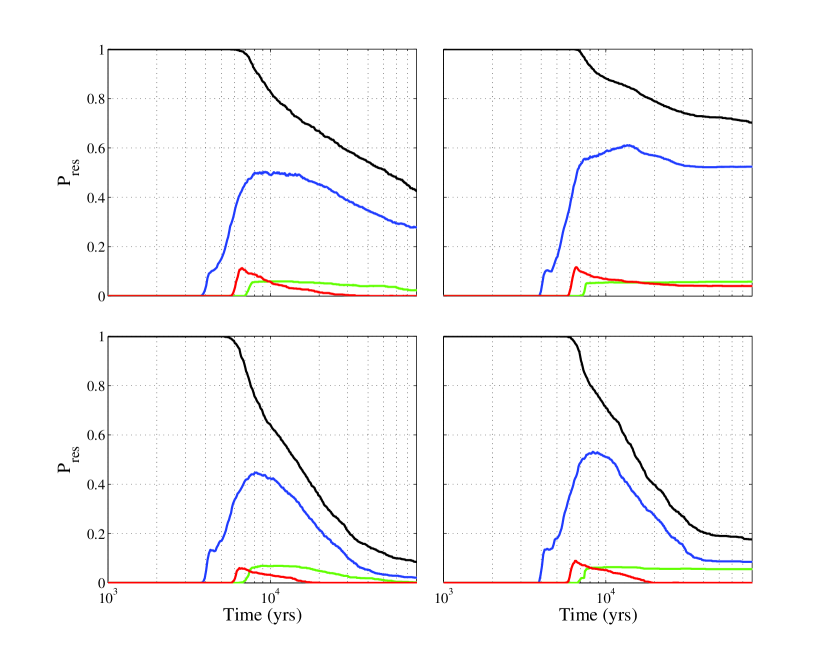
Figure 1: Fraction of systems in resonance as a function of time. Each curve shows the fraction of the ensemble that reside in 2:1 resonance (blue curve), 5:3 resonance (red curve), and 3:2 resonance (green curve) versus time. The systems are considered to be in resonance if the period ratios are near the relevant integer values and any of the resonance angles are librating (see text). The black curves shows the fraction of systems that remain intact, without losing a planet, as a function of time. For the cases shown here, the migration timescale ${\tau_{a}}$ = $2\times 10^{4}$ yr. The two panels on the top include eccentricity damping with parameter $K$ = 1; the two panels on the left include turbulence with the standard level of fluctuations (see text).

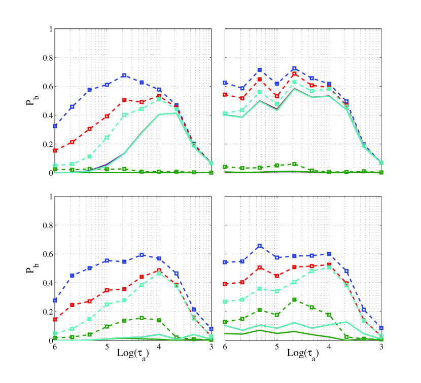
Figure 2: Fraction of systems in 2:1 resonance according to four criteria: The curves show the fraction of the ensemble that have nearly 2:1 period ratio (blue dashed curve), are in $\theta_{1}$ resonance (cyan dashed curve), are in $\theta_{2}$ resonance (red dashed curve), and are in $\theta_{3}$ resonance (green dashed curve). The heavy solid curves show the fraction of the ensemble that are in resonance (of each type) at the end of the migration epoch. Note that the fractions of $\theta_{1}$ and $\theta_{2}$ resonances at the end of the epoch are nearly identical.

2.2.1 Time Evolution and Resonance Criteria

For this set of system parameters, Figure 1 illustrates the basic time evolution for an ensemble of planetary systems. Here, the fractions of the systems that reside in mean motion resonance are plotted as a function of time for a moderately short migration timescale ${\tau_{a}}$ = $2\times 10^{4}$ yr. The simulations shown in the top panels include eccentricity damping with parameter $K$ = 1; the two panels on the left include turbulence with the standard level of fluctuations $(\Delta J)/J\sim 2\times 10^{-4}$. The various curves in each panel correspond to resonances with period ratios of 2:1 (blue), 5:3 (red), and 3:2 (green). The systems are considered to be in resonance if the period ratios are near the relevant integer values and if any of the resonance angles are librating (see Section 2.1 and equations [3 – 9]). Note that this migration rate was used because slower migration rates lead to few systems in the 5:3 and 3:2 resonances. Since all of the systems start outside of resonance, the fractions start at zero and increase with time as migration pushes the planets together. The 2:1 resonance is encountered first, so that corresponding fraction grows first. As the systems evolve, resonance is often compromised, so that the fractions reach a peak value and then decrease. After some of the systems leave the 2:1 state, they become locked into the 5:3 resonance, and then sometimes the 3:2 resonance. As a result, the peak fraction occurs later for resonances that are further inward, and the peak is lower for the weaker resonances (as expected). When systems begin to leave resonance, some of them decay by losing a planet through ejection, accretion onto the star, or collision with the other planet (the probabilities of these end states are quantified in Section 2.3). This effect is illustrated in Figure 1 by the black curves, which show the fraction of systems that retain both planets as a function of time.

We note that planetary systems are often said to “be in resonance” according to different criteria. This trend is illustrated in Figure 2 for the case of the 2:1 mean motion resonance. As shown in Figure 1, the fraction of systems that reside in resonance is a function of time for a given migration rate. The peak value of this time-dependent curve can be used as one measure of the fraction of systems that are in resonance. However, systems enter and leave resonance at different times, so that the total fraction of systems that enter resonance will be larger than the maximum fraction that reside in resonance at a given time (the peak of this curve). A necessary (but not sufficient) condition for a system to be bound into resonance is for ratio of the periods to be near 2:1. In this context, the period ratio is “near” 2:1 if $|P_{2}/P_{1}-2|\leq 0.01$, where we discuss this issue more quantitatively below. As outlined above, we first invoke the constraint that $P_{2}/P_{1}\approx 2$. This fraction is shown as the dashed blue curves marked by squares in Figure 2. The four panels show the effects of including eccentricity damping (with $K$ = 1, panels in top row) and turbulent forcing (with $(\Delta J)/J\sim 2\times 10^{-4}$, panels on left side). Next we note that each of the resonance angles can be either librating or circulating. For those that are librating, the range of angles (the libration width) is highly variable. For this paper we use the requirement that the resonance angles are confined to be within 120 degrees of the effective stability point (as defined above). With this specification, the corresponding fractions of systems in resonance are shown as the cyan curves ($\theta_{1}$ angle), the red curves ($\theta_{2}$ angle), and the green curves ($\theta_{3}$ angle). The solid curves in each panel show the fraction of systems for which any of the resonance angles are librating at the end of the migration epoch. Note that only a relatively small fraction of the systems maintain resonance for the entire migration epoch. In addition, the inclusion of eccentricity damping (top panels) is crucial for the survival of resonant states.

For completeness, we note that the curves shown in Figure 2 have slightly different meanings for the different resonance angles. In order for any one of the angles to be considered in resonance, it must librate over (approximately) three libration periods. However, these periods are not the same for the three angles. In particular, the libration period for $\theta_{3}$ is much longer than the other two. In addition, for this class of systems, the orbit of the outer (lighter) planet varies much more than that of inner Jovian planet. As a result, the argument of periastron of the outer planet can circulate on a long timescale, but the resonance angle $\theta_{2}$ can still be considered (according to the criteria used here) to be librating.

In order to understand how the period ratios vary, we monitor the period ratio for systems that are found in 2:1 mean motion resonance. Monitoring is triggered by the condition that $P_{2}/P_{1}<2.05$; however, once triggered, this bound is relaxed and the period ratio for systems in resonance can take any value as long as the angles are librating (see above). We find that systems typically exhibit both a slight offset from exact commensurability and variations about this offset. The offset is typically less than $\sim 1\%$ and the standard deviation is $\sim 2\%$. We note that offsets and variations of this magnitude are expected, given the size of the terms in the disturbing function, and hence the size of the non-Keplerian velocities due to resonance. Both the offset value and amount of variation depend on the levels of damping and turbulence, and on the duration of resonance. In the absence of turbulence, we find an offset such that $P_{2}/P_{1}\sim 2.008$. For systems that do not include eccentricity damping, the variation of the period ratio $\sigma\sim 0.04$, but decreases for systems that stay in resonance over long times (10 times the migration time scale ${\tau_{a}}$). For cases with eccentricity damping parameter $K$ = 10, the resonances are longer lasting, and we find $\sigma\sim 0.015$. For systems that include turbulent forcing, the period ratio $P_{2}/P_{1}\sim 2.007$ with $\sigma\sim 0.07$ for short lived resonances, but decreases to $P_{2}/P_{1}\sim 2.002$ with $\sigma\sim 0.015$ for longer lived resonances.

2.2.2 Resonance Survival

Figure 3 shows the effects of both turbulence and eccentricity damping on the survival of resonances as a function of migration rate. In this case, we define resonance using the requirement that the planets have nearly integer period ratios and the libration width is less than 120 degrees for any of the resonant angles. The lower right panel shows the survival of resonances as a function of migration rate with no eccentricity damping and no turbulence. This case is thus analogous to the model equations derived in Section 3 below. As expected, systems tend to leave resonance if the migration rate becomes too large. Here, systems leave the 2:1 resonance (blue curve) when the migration rate exceeds roughly $2\times 10^{-4}$ yr^-1 (${\tau_{a}}$ = 5000 yr). After leaving the 2:1 resonances, systems can become locked into the 5:3 resonance (red curve), and/or the 3:2 resonance (green curve). Note that the curve for 2:1 resonances shows a broad maximum near the migration rate of $10^{-5}$ yr^-1 (${\tau_{a}}$ = 0.1 Myr), with decreasing probability towards both slower and faster rates. The decrease with increasing migration rate is expected. The decrease toward slower migration rates occurs because some of the systems are locked into higher order resonances, which include the 7:3 and the 9:4 mean motion resonances (these fractions are not shown in the figure). With the starting period ratio of 2.4, the systems must pass through these states to reach the 2:1 resonance; with extremely slow migration rates, these weak resonances can (sometimes) survive and thus reduce the probability of the systems entering the 2:1 resonance.

The effects of including turbulent fluctuations are shown by the analogous curves in the lower left panel. Turbulence only has a chance to act on long timescales, so that the simulations with long migration times (low migration rates) are affected the most. More specifically, for migration rates slower than about $10^{-5}$ yr^-1 (${\tau_{a}}$ = 0.1 Myr), turbulence has time to act, and the probability of maintaining a resonant configuration is lower, as shown on the left hand side of the plot. We note that with the inclusion of turbulence, the weak higher order resonances (7:3 and 9:4) generally do not survive (unlike the case of no turbulence in the lower right panel).

The effects of including eccentricity damping is shown by the top right panel, where we have taken $K$ = 1 (so that eccentricity is damped on the same timescale that migration takes place; see equation [2]). The inclusion of this damping effect acts to preserve resonance – note that all of the survival fractions are higher when ${\dot{e}}\neq 0$ than in the absence of damping. This effect is especially important for the long-term survival of the resonant states (compare the solid curves in the top panels with those in the bottom panels), especially for the case of the 2:1 resonance. The survival probabilities of the (weaker) 5:3 and 3:2 resonances are also enhanced by the inclusion of eccentricity damping, but the absolute values of these probabilities remain low. Keep in mind that these results correspond to $K$ = 1; larger eccentricity damping rates lead to more dramatic consequences (see below).

When both turbulent forcing and eccentricity damping are included, we obtain the results shown in the upper left panel of Figure 3. In this case, the effects of turbulence dominate at low migration rates, so that fewer resonant systems survive. At high migration rates, however, turbulence does not have sufficient time to act and the effects of eccentricity damping lead to a net gain in the survival fractions. For migration rates faster than about $3\times 10^{-5}$ yr^-1 (${\tau_{a}}\approx 0.033$ Myr), eccentricity damping dominates over the effects of turbulence, so that more resonant systems survive.

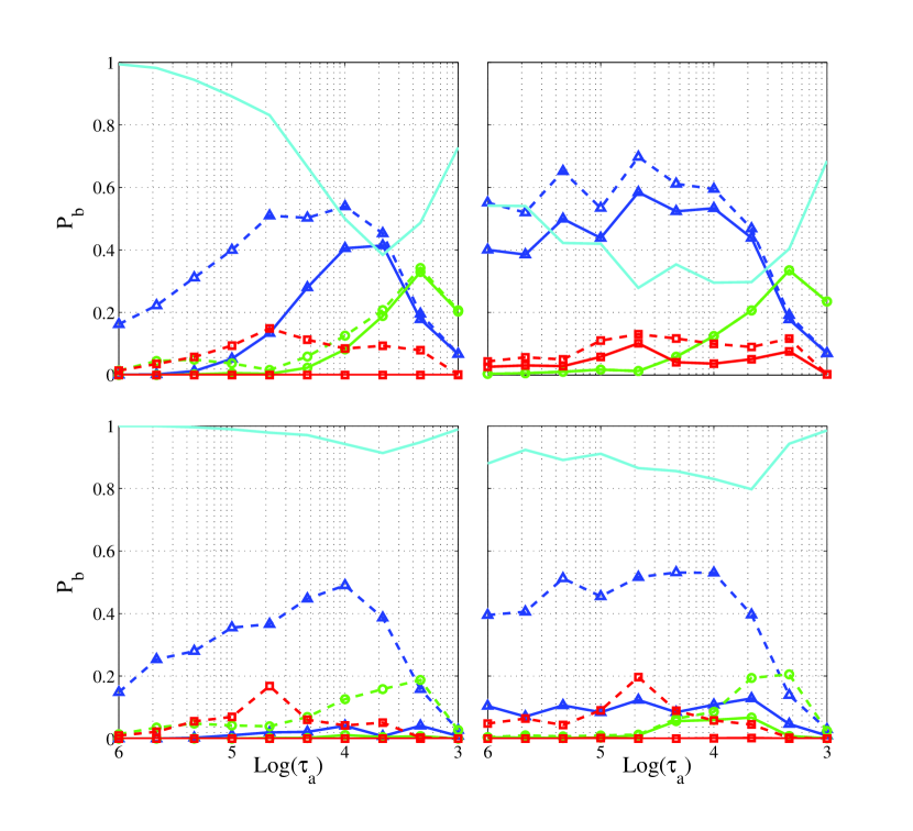
Figure 3: Effects of eccentricity damping and turbulent forcing on the survival of mean motion resonances for a two planet system. The inner planet has mass $m_{1}=1{M_{J}}$, and the outer planet has mass $m_{2}=10{M_{\earth}}$. The two panels in the left column include turbulent forcing. The panels in the top row include eccentricity damping, which acts on the same timescale as the migration rate (eccentricity damping parameter $K$ = 1). The lower right panel shows the results with migration only. The dashed curves show the fraction of systems that enter into mean motion resonance as a function of migration rate (${\tau_{a}}$ measured in yr), where this fraction is measured using the peak value (as a function of time – see the curves of Figure 1). The solid curves show the fraction that remain in resonance at the end of the migration epoch. The colors denote the various resonances, including the blue curve marked by triangles (2:1), red curve marked by squares (5:3), and green curve marked by circles (3:2). The upper cyan curve shows the fraction of systems that are not in resonance at the end of the simulations.

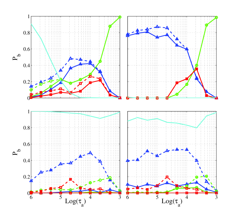
Figure 4: Effects of eccentricity damping and turbulent forcing on the survival of mean motion resonances for a two planet system with eccentricity damping parameter $K$ = 10. Other properties are the same as in Figure 3: The planet masses are $m_{1}=1{M_{J}}$ and $m_{2}=10{M_{\earth}}$. The panels in the left column include turbulent forcing. The panels in the top row include eccentricity damping with $K$ = 10. The lower right panel shows the results with migration only. The dashed curves show the fraction of systems that enter into mean motion resonance as a function of migration rate. The solid curves show the fraction that remain in resonance at the end of the migration epoch. The colors denote the various resonances, including the blue curve marked by triangles (2:1), red curve marked by squares (5:3), and green curve marked by circles (3:2). The upper cyan curve shows the fraction of systems that are not in resonance at the end of the simulations.

For comparison, we consider the survival of resonant systems for the case with eccentricity damping parameter $K$ = 10. These results are shown in Figure 4, where all of the system parameters are the same as in Figure 3 except for the larger rate of eccentricity damping. As expected (e.g., Lecoanet et al. 2009), the simulations with $K$ = 10 result in a larger survival rate than the corresponding cases with $K$ = 1 (compare the upper right panels of Figures 4 and 3). For slower migration rates, where the dominant outcome is the 2:1 resonance (blue curves), the survival rate increases only modestly, from $P_{b}\sim 0.6$ to $P_{b}\sim 0.8$ with increasing values of $K$ (for the case with no turbulence). For higher migration rates, the 3:2 resonance is most common state, and the survival rate increases substantially for the $K$ = 10 case (compared to $K$ = 1 systems). For the simulations that include turbulent fluctuations, however, the differences in survival fractions for the 2:1 resonance between the $K$ = 10 and $K$ = 1 cases are minimal (compare the upper left panels of Figures 3 and 4). In the absence of turbulence, the increase in resonance survival (for larger $K$) arises most strongly at slow migration rates; however, the regime of slow migration is where turbulence has enough time to act, and hence to compromise resonant states. For 3:2 resonances, which arise primarily at fast migration rates where turbulence does not have enough time to act, the increased eccentricity damping rate leads to substantially larger survival fractions.

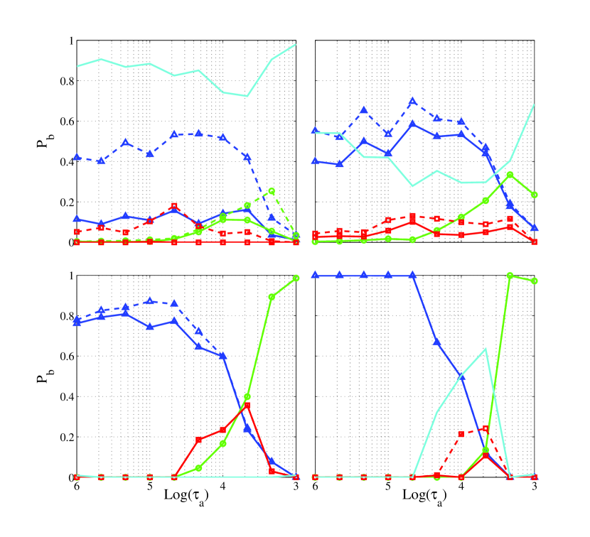
Figure 5: Effects of eccentricity damping on the survival of mean motion resonance. This two-planet system has planetary masses of $m_{1}=1{M_{J}}$ and $m_{2}=10{M_{\earth}}$. The four panels show the survival fractions as a function of migration rate for increasing values of the eccentricity damping parameter $K$ where ${\dot{e}}/e$ = $K{\dot{a}}/a$. Results are shown for $K$ = 0.1, 1, 10, and 100, where the $K$ values increase from upper left to lower right. In each panel, the curves correspond to various resonances, including the blue curve marked by triangles (2:1), red curve marked by squares (5:3), and green curve marked by circles (3:2). The unmarked cyan curve shows the fraction of systems that are not found in any of the mean motion resonances. The solid curves show the fraction of systems in resonance at the end of the migration epoch; the dashed curves show the largest value of the fractions during the migration epoch.

Before leaving this section, we note that the simulations shown thus far all start with the planets confined to the orbital plane. In order to see how nonzero inclination angles affect the results, we have carried out a series of test simulations where the planets are given non-zero displacements in the vertical dimension in their starting states (so that these simulations are fully three-dimensional). The results of these test simulations indicate that the third dimension is unimportant as long as the initial departures from the plane are not too large. More specifically, the starting vertical coordinates $z_{0}$ are uniformly sampled within the range $[-H,H]$, where $H$ is the scale height of the disk. These test simulations use a variety of scale heights, with $H/r$ = 0, 0.05, 0.10, and 0.20; we also use a 10 ${M_{\earth}}$ outer planet, eccentricity damping parameter $K$ = 10, and our standard level of turbulence. For this choice of parameters, the results are virtually unchanged.

2.2.3 Effects of Eccentricity Damping and Turbulence

Next we consider the case of eccentricity damping acting alone. Figure 5 shows the survival probabilities as a function of migration rate for four values of the eccentricity damping timescale, where the parameter $K$ = 0.1, 1, 10, and 100. Taken together, the four panels of Figure 5 show that eccentricity damping acts to increase the fraction of systems that remain in mean motion resonance. The effect is most pronounced for the 2:1 resonance, and for slow migration rates. In the regime of slow migration, a significant fraction of the systems leave the 2:1 resonance, presumably through the excitation of eccentricity via planet-planet interactions (Adams & Laughlin 2003, Moorhead & Adams 2005, Chatterjee et al. 2008, Ford & Rasio 2008, Matsumura et al. 2010). The inclusion of eccentricity damping counteracts this excitation and allows more systems to remain in resonance.

For sufficiently large eccentricity damping rates (characterized by $K$ = 100), essentially all systems remain in 2:1 resonance until the migration rate exceeds a well-defined value, found numerically to be $|{\dot{a}}|/a\sim 3\times 10^{-5}$ yr^-1 or ${\tau_{a}}\approx 0.033$ Myr (shown in the lower right panel of Figure 5). These results show that the loss of resonant states for the other cases (5:3 and 3:2) also occurs at well-defined values of the migration rate. In addition, as a rough approximation, the migration rates at which these three resonances are compromised are found to be evenly spaced logarithmically (by factors of $\sim 3$). This behavior can be understood in a qualitative manner through simple physical considerations (see below) and through model equations (Section 3). Finally, we note that the 5:3 resonance, which is second order and hence weak, is sparsely populated; as a result, many of the systems with migration time scales $\sim 3000$ yr are not found in any resonance.

The basic clock that determines the dynamics of these planetary systems is set by the libration timescale of the resonance. For the simplest model of the resonance, that resulting from the circular restricted three-body problem, the frequency for external resonances is given by

$$\omega_{0}^{2}=-3j_{1}^{2}{\cal C}_{R}ne^{|j_{3}|}\qquad{\rm where}\qquad{\cal C}_{R}=\left({m_{P}\over M_{\ast}}\right)n\left[f_{d}(\alpha)+\alpha^{-1}f_{i}(\alpha)\right]\,,$$ (10)

where $n$ is the mean motion of the outer planet, $\alpha$ = $a_{1}/a_{2}$, and the functions $f_{d}(\alpha)$ and $f_{i}(\alpha)$ are given by the Laplace coefficients (see §8.5 of MD99). For odd order resonances, the function $f_{d}<0$, so that the corresponding frequencies are real. For even order resonances, $f_{d}>0$, but the equilibrium angle is shifted by $\pi$, and the frequencies are again real (see MD99 for further discussion). Notice also that $f_{i}$ is nonzero only for the 2:1 resonance. The integers $j_{1}$ and $j_{3}$ depend on the type of resonance. Although both integers are negative for the cases of interest, the libration timescale only depends on the absolute value. More specifically, the integer pair $(|j_{1}|,|j_{3}|)$ takes on the values (1,1), (3,2), and (2,1) for the 2:1, 5:3, and 3:2 resonances, respectively. For the values $e$ = 0.10 and $\mu=m_{P}/M_{\ast}=10^{-3}$, as used in the numerical simulations, we find that $\omega_{0}^{2}/(3\mu en^{2})\approx$ 2.0, 3.0, and 8.1 for the three resonances. For these parameter values, the square of the frequencies are spaced by factors of $\sim 2$. This simple analytic result is thus in qualitative, but not quantitative, agreement with the numerical results. One should keep in mind that the orbital elements that enter into these formulae (e.g., $e$ and $n$) vary over the course of the simulations, so that comparisons are complicated.

If the migration rate ${\dot{a}}/a$ were the only relevant variable, then one would expect that capture into resonance would be compromised at a fixed value of the dimensionless parameter $a\omega_{0}$ / $|{\dot{a}}|=\omega_{0}{\tau_{a}}$. The case that most closely meets this expectation is that of migration with no eccentricity damping and no turbulent forcing (shown in the lower right panel of Figure 3). For this class of simulations, systems tend to enter the 3:2 resonance states for higher migration rates than for the 2:1 resonances, where this trend is predicted (qualitatively) by the simple theory outlined above. However, the fraction of systems in 5:3 resonance is not larger than the fraction in 2:1 resonance at large migration rates, in spite of the 5:3 having a shorter libration period. The 5:3 resonance is generally weaker, in the sense of being easier to disrupt, than the first order resonances, and does not survive for large migration rates. In terms of survival of the resonances, shown by the solid curves, the fraction in 2:1 is generally larger for all migration rates due to its greater stability.

For the case of migration with large eccentricity damping rates (see the lower right panel of Figure 5), the probability of resonance survival shows the expected qualitative behavior: Each of the resonances dominates (has the largest fraction) for a well-defined range of migration rates. The 2:1 resonance is by far the most important for migration timescales longer than about $10^{4}$ yr. For shoter timescales, there is a narrow window of migration rates where the fraction of systems in 5:3 resonance shows a peak, and then the 3:2 resonance dominates for faster migration rates. Although the ordering of these results is consistent with theoretical expectations, the maximum migration rates are spaced at larger intervals than the factors of $\sqrt{2}$ suggested by the above analysis. Here, the large eccentricity damping rates significantly change the dynamics and hence the numerical values. Nonetheless, the qualitative trend holds up.

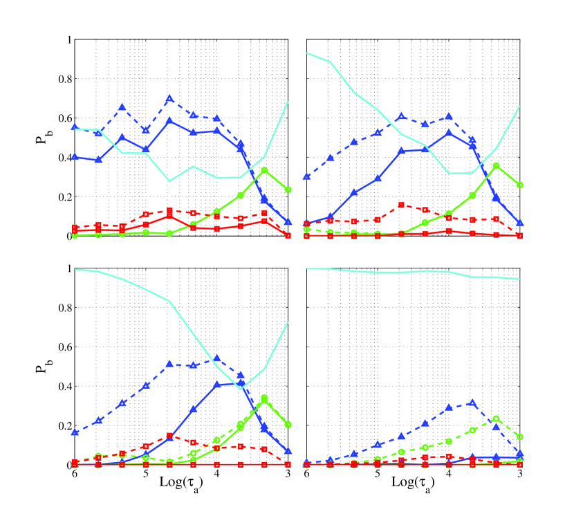
Figure 6: Effects of increasing turbulence on the survival of mean motion resonance. This two-planet system has planetary masses of $m_{1}=1{M_{J}}$ and $m_{2}=10{M_{\earth}}$. The four panels show the survival fractions as a function of migration rate for increasing levels of turbulence, as specified by the forcing strength $[(\Delta J)/J]_{k}$ per independent realization of the turbulent fluctuations. Results are shown for $[(\Delta J)/J]_{k}$ = 0 (no turbulence), $10^{-4}$, $3\times 10^{-4}$, and $10^{-3}$, where turbulence increases from upper left to lower right. In each panel, the curves correspond to various resonances, including the blue curves marked by triangles (2:1), red curves marked by squares (5:3), and green curves marked by circles (3:2). The unmarked cyan curves show the fraction of system that are not found in any of the mean motion resonances. The solid curves show the fraction of systems in resonance at the end of the migration epoch; the dashed curves show the largest value of the fractions during the migration epoch. The eccentricity damping parameter $K$ = 1 for these simulations.

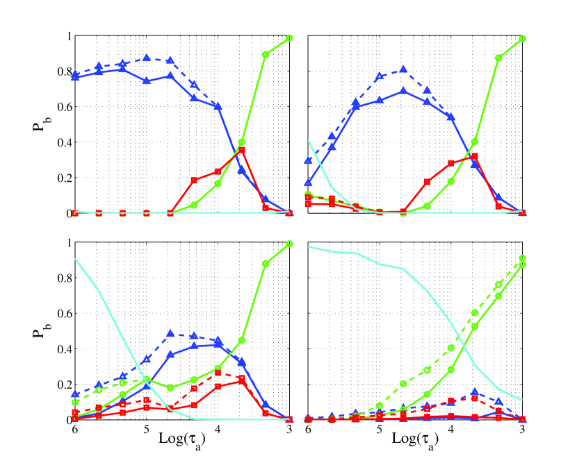
Figure 7: Effects of increasing turbulence on the survival of mean motion resonance for systems with eccentricity damping parameter $K$ = 10. Other system properties are the same as in Figure 6. This system has planet masses $m_{1}=1{M_{J}}$ and $m_{2}=10{M_{\earth}}$. The four panels show the survival fractions as a function of migration rate for increasing levels of turbulence. Results are shown for forcing strength $[(\Delta J)/J]_{k}$ = 0, $10^{-4}$, $3\times 10^{-4}$, and $10^{-3}$, where turbulence increases from upper left to lower right. In each panel, the curves correspond to various resonances, including the blue curves marked by triangles (2:1), red curves marked by squares (5:3), and green curves marked by circles (3:2). The unmarked cyan curves show the fraction of system that are not found in any of the mean motion resonances. The solid curves show the fraction of systems in resonance at the end of the migration epoch; the dashed curves show the largest value of the fractions during the migration epoch.

As the levels of turbulence increase, systems have greater difficulty maintaining mean motion resonance. This trend is quantified by the simulations depicted in Figures 6 and 7. These numerical experiments are carried out using the standard case of a Jovian planet on the inside and an inward migrating “super-earth” with mass $m_{2}$ = 10 ${M_{\earth}}$. The eccentricity damping rate is set at the standard values of $K=1$ (Figure 6) and $K=10$ (Figure 7). As the amplitude of the turbulent fluctuations increases (from upper left to lower right in both Figures), the general trend is for the fraction of systems in resonance to decline significantly. The 2:1 mean motion resonance, which is the strongest and the first to be encountered, is compromised for sufficiently rapid migration rate. As the level of turbulence increases, the migration rate at which systems leave the 2:1 resonance becomes lower (the curves shift to the right in the figures). We also note that the destructive action of turbulence is more pronounced for the solid curves, i.e., for the fraction of systems that remain in resonance at the end of the migration time. Finally, as expected, we find that more resonant systems survive for larger rates of eccentricity damping (compare Figures 6 and 7).

With the initial conditions used herein, where the planets are started outside the 2:1 resonance, the faster 5:3 and 3:2 resonances are not affected as severely by the presence of turbulence. These other resonances only arise when the migration rate is rapid, so that the migration timescale is short and turbulence has little time to act. For the 5:3 and 3:2 resonances, the probability curves shown in Figure 6 decrease slowly with increasing turbulent amplitude. As expected, the largest effect arises for the largest turbulent amplitude $[(\Delta J)/J]_{k}$ = $10^{-3}$, where the probability of remaining in any of the resonant states is extremely low at the end of the migration epoch; the fraction of systems not bound into resonance is marked by the solid cyan curve, which is close to unity for all migration rates. Note that the 3:2 resonance lasts the longest in the face of increasing turbulence. This apparent resilience arises because the 3:2 cases are only present for fast migration rates, the regime where turbulence has less time to act (it is not due to the increased durability of the resonance).

2.2.4 Equal Mass Planets

Next we consider the case of two equal mass planets, with $m_{1}$ = $m_{2}$ = ${M_{J}}$. The results for survival of mean motion resonance are shown in Figure 8. The panels on the left include the effects of turbulent forcing; the panels on the top include the effects of eccentricity damping, where the parameter $K$ = 1 so that the eccentricity damping timescale is the same as the migration timescale. These results for two Jovian planets are significantly different than those shown in Figure 3 for the case of a lower mass outer planet. One important effect of higher planetary masses is to increase the levels of planet-planet interactions in the systems. This effect, in turn, leads to greater libration widths for systems that stay in resonance and a lower probability of remaining in a resonant state. As a result, the probability of the system residing in either the 5:3 or the 3:2 resonance is significantly lower than in the case of a less interactive system (compare Figures 3 and 8). On the other hand, the fraction of systems that remain in the 2:1 resonance is larger for the more interactive (two jupiter) systems.

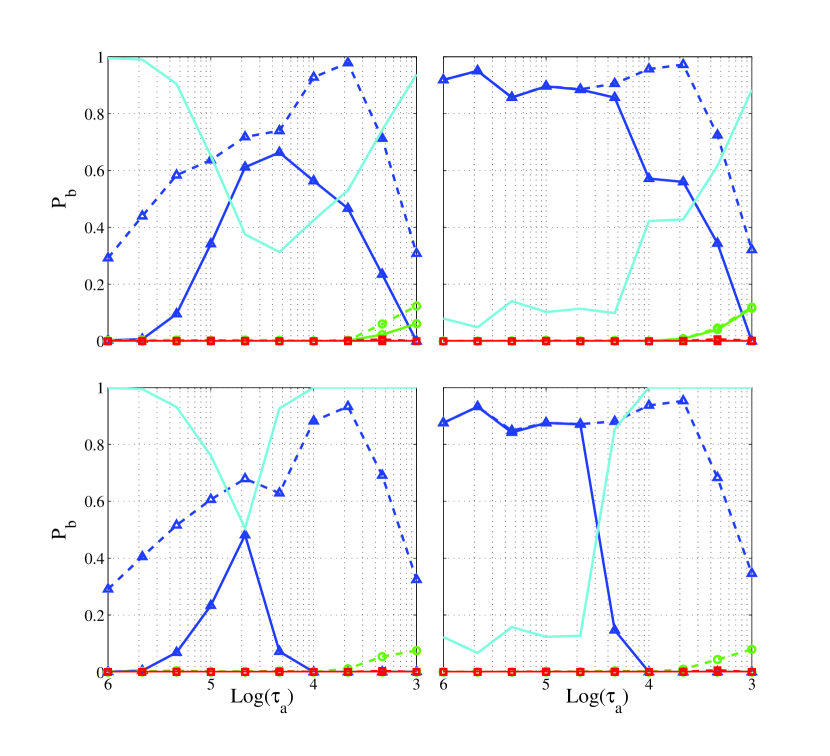
Figure 8: Effects of eccentricity damping and turbulent forcing on the survival of mean motion resonances for planetary systems containing two Jovian planets ($m_{1}=m_{2}=1{M_{J}}$). The panels on the left include turbulent forcing; the top panels include eccentricity damping (where the eccentricity damping parameter $K$ = 1). The lower right panel shows the results with migration only. All of the panels show the fraction of systems that remain bound in mean motion resonance as a function of migration time scale (measured in yr). The curves correspond to various resonances, including the blue curves marked by triangles (2:1), red curves marked by squares (5:3), and green curves marked by circles (3:2). The unmarked cyan curve shows the fraction of system that are not found in any of the mean motion resonances. Solid curves show the fractions at the end of the migration epoch; dashed curves show the peak values of the fractions during the migration epoch.

2.3 End States

During the course of the numerical integrations, the planetary systems can end their evolution in a variety of ways. In many cases, the systems remain bound together, even though mean motion resonance is often compromised as described above. In many other cases, however, planets can be lost through scattering encounters, through collisions with each other, or via accretion onto the central star. This section outlines the probabilities for each of these possible end states of these dynamical systems.

Figure 9: Probability of the planetary systems evolving into varying end states for planet masses $m_{1}=1{M_{J}}$ and $m_{2}=10{M_{\earth}}$. Each panels shows the fraction of the systems that end their evolution with a given end state, plotted here as a function of migration rate. The end states represented here include survival of both planets (black curves), planetary collisions (blue curves), ejection of a planet (green curves), and accretion of a planet by the central star (red curves). Four ensembles of simulations are depicted for migration only (lower right panel), migration and eccentricity damping (with $K$ = 1; upper right), migration and turbulence (lower left), and all three effects (upper left).

For eccentricity damping parameter $K$ = 1, Figure 9 shows the likelihood of the planetary systems ending their evolution in various possible end states for the standard case with inner planet mass $m_{1}=1{M_{J}}$ and outer planet mass $m_{2}=10{M_{\earth}}$. These probabilities are shown as a function of migration rate for ensembles of simulations with migration only, migration and eccentricity damping, migration and turbulence, and for simulations including all three effects. The evolution of these systems produces a wide variety of outcomes, including survival of both planets for the entire evolutionary time (shown by the black curves), ejection of a planet (green curves), accretion by the central star (red curves), and collisions between the planets (blue curves). As illustrated by the four panels in the figure, the corresponding probabilities depend sensitively on the migration rates, eccentricity damping rates, and the levels of turbulence.

Figure 9 shows several trends. In general, the probability for both planets to survive tends to decrease with increasing values of the migration rate. This trend is expected, because slow migration rates allow the systems to adjust as they evolve; these cases with slow migration systematically exhibit less overall action than cases with higher migration rates. One important exception to this trend arises for the case of slow migration rates, the inclusion of turbulent fluctuations, and no eccentricity damping (see the lower left panel in Figure 9). In this regime, migration time scales are long enough that turbulence has time to act, which leads to loss of mean motion resonance (see the previous section), a greater possibility of orbit crossing, and subsequent planetary ejection. For this class of systems, the outer planet has substantially less mass than the inner planet and is far more susceptible to being lost. The outer planet is removed through ejection, accretion onto the central star, and through collisions with the inner Jovian planet. Note that the first two of these channels dominate the third.

Figure 9 shows another trend: As the migration rate increases, the probability of losing a planet through ejection decreases, whereas the probability of losing a planet through accretion onto the star increases. One important physical property that determines the relative number of accretion events versus ejections is the location of the planet(s) in the gravitational potential well of the star at the end of the migration epoch (when the planets are likely to suffer close encounters). The depth of the stellar potential well at $a$ = 1 AU is approximately (30 km/s)², whereas the depth of the potential well at the surface of Jupiter is (43 km/s)². These scales are thus comparable. For fast migration rates, the outer planet is able to push the inner planet somewhat farther inward, deeper into the stellar potential well, and hence the probability of ejection decreases.

Figure 10 shows the analogous plots for the channels of planetary loss for systems initially containing two Jovian planets ($m_{1}=m_{2}=1{M_{J}}$). The trends are roughly similar to the case with lower mass outer planets: Planetary survival decreases with increasing migration rate. Turbulence leads to planetary loss in the regime of slow migration and no eccentricity damping, where the regime of slow migration corresponds to migration time scales longer than about ${\tau_{a}}$ = $3\times 10^{4}$ yr. And, as the migration rate increases, there is a shift from loss of planets through ejection to a loss of planets through accretion onto the central star. However, for these systems with two Jovian planets, ejections, collisions, and accretion events are on a more equal footing. One clear difference from the case of low-mass outer planets is that planet-planet collisions are more common (compare the blue curves in Figures 9 and 10). The other significant difference is that the inner planet is more often lost during accretion events, rather than the outer planet (shown by the dotted curves in Figure 10).

For solar systems with sufficiently large values of the eccentricity damping parameter $K$, most of the planets survive over the relatively short timescales considered in this paper. For example, for cases with $K$ = 10, most systems remain intact and neither eject nor accrete a planet. However, as shown by the comparison of Figures 3 and 4, the fraction of systems that remain in mean motion resonance for $K$ = 10 is only moderately increased over the values obtained for $K$ = 1. The solar systems that are not in resonance will often eject or accrete planets on longer timescales, even in the absence of additional migration (e.g., Holman & Wiegert 1999; David et al. 2003). This issue should be addressed with additional, longer term numerical integrations, but is beyond the scope of this present work.

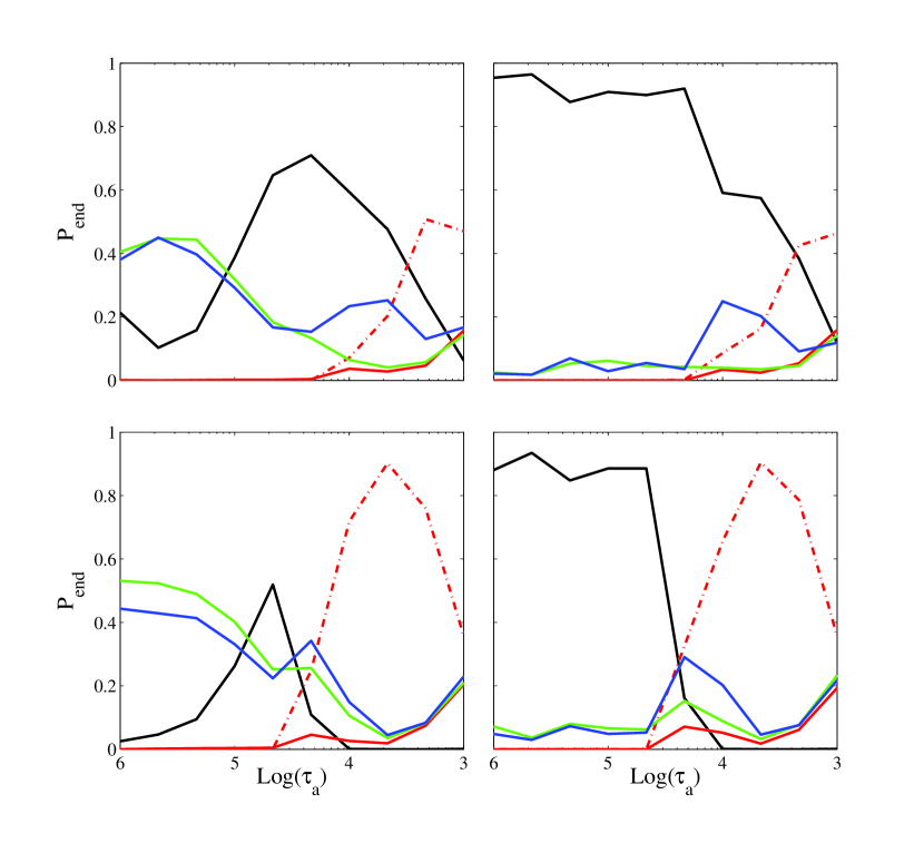
Figure 10: Probability of the planetary systems evolving into varying end states for planet masses $m_{1}=m_{2}=1{M_{J}}$. Four ensembles of simulations are depicted for cases with migration only (lower right panel), migration and eccentricity damping (upper right), migration and turbulence (lower left), and all three effects (upper left). The end states represented here include survival of both planets (black curves), planetary collisions (blue curves), ejection of a planet (green curves), and accretion of a planet by the central star (red curves).

3 MODEL EQUATIONS

In this section we derive a Hamiltonian model to describe the migration of a pair of planets into mean motion resonance. In this context, we want to find the simplest possible set of model equations that captures the essential physics. Toward this end, we make a number of simplifying assumptions. In particular, most of this discussion is restricted to the case of a single resonance, which we take to be the 2:1 mean motion resonance; note that other resonances can be considered in similar fashion. In qualitative terms, this analysis should apply to the variety of resonances that we consider in the numerical simulations of Section 2. The development is parallel to previous treatments (Quillen 2006, Friedland 2001).

3.1 Derivation

As a starting point, we consider a test particle of mass $m_{0}$ orbiting in the same plane as a larger planet with mass $m_{P}$, which is orbiting a star of mass $M_{\ast}$. The masses thus obey the ordering

$$m_{0}\ll m_{P}\ll M_{\ast}\,.$$ (11)

The orbital elements of the test particle are as follows: $\lambda$ is the mean longitude, $M$ is the mean anomaly, $a$ is the semi-major axis, $\varpi$ is the longitude of pericenter, and $e$ is the orbital eccentricity. The analogous variables for the planet have the same symbols but are denoted with the subscript ‘$P$’ (see below). The Poincaré coordinates (MD99) can be written

$$\lambda=M+\varpi\qquad{\rm and}\qquad{{\widetilde{\gamma}}}=-\varpi\,,$$ (12)

with momentum variables of the form

$$\ell=(GM_{\ast}a)^{1/2}\qquad{\rm and}\qquad\Gamma=(GM_{\ast}a)^{1/2}\left[1-(1-e^{2})^{1/2}\right]\,.$$ (13)

The Hamiltonian can be written in the form

$$H=-{(GM_{\ast})^{2}\over 2\ell^{2}}-{{\cal R}}\,,$$ (14)

where ${{\cal R}}$ is the disturbing function due to the gravitational interaction between the test particle and the planet.

Specializing to the case of a 2:1 mean motion resonance where the planet is the inner body, we perform a canonical transformation using the generating function

$$F_{2}=I(2\lambda-\lambda_{P})\,,$$ (15)

which leads to the new variables

$$I=-\ell/2\qquad{\rm and}\qquad\psi=\lambda_{P}-2\lambda\,.$$ (16)

The new Hamiltonian for the unperturbed problem, without the disturbing function, has the form

$$H_{0;new}=-{(GM_{\ast})^{2}\over 8I^{2}}-In_{P}\,,$$ (17)

where $n_{P}$ is the mean motion of the planet.

Next we express all quantities in dimensionless form and expand around the resonance. Here, distances are measured in units of the semimajor axis $a$, time is measured in units of $(a^{2}/GM_{\ast})^{1/2}$, and mass is measured in units of $M_{\ast}$. If we define

$$\delta\equiv I-I_{0}\qquad{\rm and}\qquad{1\over 4I_{0}^{3}}=n_{P}(t_{0})\,,$$ (18)

the new Hamiltonian now reads

$$K_{0;new}={constant}-(n_{P}-1)\delta-{3\delta^{2}\over 8I_{0}^{4}}\,.$$ (19)

We must now include the relevant terms from the disturbing function, which provides an expansion in orders of eccentricity (of both the test mass and the planet). Here we keep only the leading order term (see MD99 and Quillen 2006) and write the Hamiltonian (from equation [19]) in the form

$$K(\delta,\psi,\Gamma,{{\widetilde{\gamma}}})=-6\alpha^{2}\delta^{2}-(n_{P}-1)\delta-2\mu f_{2}\alpha^{1/2}\Gamma+A\Gamma^{1/2}\cos(\psi-\varpi)\,,$$ (20)

where $A$ is the expansion coefficient in the disturbing function and where we have used the fact that $I_{0}$ = $\alpha^{-1/2}/2$ for these units and choice of resonance.

Following Quillen (2006), we perform another canonical transformation using the generating function

$$F_{2}=J_{1}(\psi-\varpi)+J_{2}\psi\,,$$ (21)

which leads to the new variables

$$J_{1}+J_{2}=\delta\,,\qquad\phi=\psi-\varpi\,,\qquad J_{1}=\Gamma\,,\qquad{\rm and}\qquad\theta=\psi\,,$$ (22)

and hence the new Hamiltonian

$$H=-6\alpha^{2}\left(\Gamma^{2}+J_{2}^{2}\right)-\left[12\alpha^{2}J_{2}+(n_{P}-1)+2\mu f_{2}\alpha^{1/2}\right]\Gamma-(n_{P}-1)J_{2}+A\Gamma^{1/2}\cos\phi\,.$$ (23)

Since $J_{2}$ is conserved and constant terms can be dropped, the Hamiltonian can be simplified to the form

$$H=6\alpha^{2}\Gamma^{2}+\left[12\alpha^{2}J_{2}+(n_{P}-1)+2\mu f_{2}\alpha^{1/2}\right]\Gamma-A\Gamma^{1/2}\cos\phi\,.$$ (24)

Next we rescale the momentum variable $\Gamma$ according to the transformation

$$\Gamma\to\left[{6\alpha^{2}\over A}\right]^{2/3}\Gamma\,,$$ (25)

and rescale the time variable so that the Hamiltonian $H$ is given by

$$H=\Gamma^{2}+b\Gamma-\Gamma^{1/2}\cos\phi\,.$$ (26)

The parameter $b$ is thus given by

$$b=\left[12\alpha^{2}J_{2}+(n_{P}-1)+2\mu f_{2}\alpha^{1/2}\right]6^{-1/3}(\alpha A)^{-2/3}\,.$$ (27)

The first and third terms in square brackets are generally small compared to unity. The central term vanishes on resonance, by definition, but can be of order unity when the system is far from resonance. As a result, the parameter $b$ provides a measure of how far the system resides from a resonant condition. For this paper, we let the parameter $b$ evolve linearly with time so that the systems approach resonance ($b$ = 0) at a well-defined rate.

Using the Hamiltonian with the form given by equation (26), the equations of motion become

$${d\Gamma\over dt}=-\Gamma^{1/2}\sin\phi\,,$$ (28)

and

$${d\phi\over dt}=2\Gamma+b-{1\over 2\Gamma^{1/2}}\cos\phi\,.$$ (29)

It is useful to define the reduced momentum variable $p\equiv\Gamma^{1/2}$ so that the equations of motion simplify to the forms

$$2{dp\over dt}=-\sin\phi\,,$$ (30)

and

$${d\phi\over dt}=2p^{2}+b-{1\over 2p}\cos\phi\,.$$ (31)

Although this ansatz simplifies the equations of motion, note that the variables $(\phi,p)$ are no longer canonical. We also note that this change of variables in convenient for calculating curves in phase space to analyze the dynamics (this exercise is carried out in the Appendix).

Figure 11: Time evolution of the resonance angle for a model system that becomes trapped in resonance. The top panel shows the variable $\sin[\phi(t)]$ versus time, for a starting value of $\Gamma_{0}$ = 0.01 and a migration rate $db/dt$ = –0.1. The bottom panel shows the time evolution of the momentum variable $\Gamma$.

3.2 Entry into Resonance

Using the model equations derived above, we can study the entry into mean motion resonance as a function of the normalized migration rate $db/dt$. Here, the initial conditions are given by the starting momentum $\Gamma_{0}$ and the starting value of the angle $\phi$. We choose fixed values of the momentum variable $\Gamma_{0}$ and then study the probability of entering into resonance as a function of migration rate $db/dt$. Since these systems often display extreme sensitivity to their starting conditions, we must perform many realizations of the numerical integrations for each pair $(\Gamma_{0},db/dt)$, where each realization uses a different value of the starting angle $\phi$. For the sake of definiteness, we start the systems with $b=b_{0}$ = 10 (well outside of resonance) and let the resonance parameter evolve according to the relation $b(t)=b_{0}-(db/dt)t$. The systems thus pass through resonance at time $t=b_{0}/|db/dt|$.

One example integration is shown in Figure 11, which plots the quantity $\sin\phi$ (top panel) and the momentum variable $\Gamma$ (bottom panel) as a function of time for a system that becomes locked into mean motion resonance. In this case, the libration width of the system steadily decreases with time until it reaches a steady state near time $t$ = 100 (in dimensionless units). In this case, $db/dt$ = 0.1, so that $t\sim 100$ corresponds to the time when the system passes through resonance (as expected). The momentum variable $\Gamma$ stays small until the system enters resonance, and then grows steadily (see also the discussion of Quillen 2006).

Figure 12: Fraction of systems that survive in mean motion resonance as a function of migration rate $db/dt$. The three curves correspond to different initial conditions, where the the angular momentum variable $\Gamma_{0}$ = 0.1 (top curve), 1 (center curve), and 3 (bottom curve). Each point on each curve shows the result of 1000 realizations of the evolution, each with a randomly chosen starting angle. Note that this model system corresponds to the case of the 2:1 mean motion resonance.

As found previously (Quillen 2006), the probability of entering and surviving in resonance decreases with increasing migration rate. This trend is illustrated in Figure 12, which shows the probability of achieving a resonant state versus the migration rate $db/dt$. The three curves shown in the figure use different starting values of the momentum variable $\Gamma_{0}$ = 0.1, 1, and 3. Recall that $\Gamma$ is related to the orbital eccentricity of the migrating planet (equation [13]). Previous work shows that small starting momentum generally leads to resonance capture, whereas larger values generally do not (Quillen 2006); the value $\Gamma_{0}$ = 1 corresponds to the transition region. For each value of the rate $db/dt$, we have performed an ensemble of 1000 integrations, each with a different starting value of the angular variable $\phi$. The probability of capture decreases with increasing $db/dt$, but the curves show a great deal of additional structure. The probability of achieving resonance decreases near $db/dt$ = 1 and approaches zero for somewhat larger values $db/dt\sim 3-5$.

Another clear trend is that increasing the initial value of the momentum variable $\Gamma_{0}$ acts to decrease the probability of entering into resonance. In other words, larger eccentricities tend to compromise the chances of attaining resonance. This finding is consistent with the full numerical integrations of the previous section, where eccentricity damping was found to allow for more resonant states (see Figure 5).

The leading order trend illustrated by Figure 12 is that resonant capture is more difficult with fast migration. This result, obtained from the model equations of this section, is thus consistent with the results of the numerical simulations of Section 2 (see Figures 2 – 8). We can understand this effect through a simple analysis: In the limit of large $db/dt=\gamma$, which we consider to be a constant, the equation of motion for $\phi$ simplifies to the form

$${d\phi\over dt}=-\gamma t\qquad\Rightarrow\qquad\phi=-{1\over 2}\gamma t^{2}\,,$$ (32)

where we have used the same sign convention as before. The momentum variable is then given by the remaining equation of motion, which can be written in integral form

$$p-p_{0}={1\over 2}\int\sin\left({1\over 2}\gamma t^{2}\right)dt={1\over(2\gamma)^{1/2}}\int\sin u^{2}du={1\over 2}\left({\pi\over\gamma}\right)^{1/2}S\left[\left({\gamma\over\pi}\right)^{1/2}t\right]\,,$$ (33)

where $S(z)$ is the Fresnel integral (e.g., Abramowitz & Stegun 1965). In the limit $z\to\infty$, $S(z)\to 1/2$, so the expression on the right hand side of equation (33) approaches a constant value $(\pi/16\gamma)^{1/2}$. As result, the momentum variable $p$ approaches a constant, and hence does not grow, so the system does not enter resonance. For a given starting value of the momentum variable $\Gamma_{0}$, the critical value of the migration rate $\gamma$ can be estimated by

$$\gamma_{c}={\pi\over 16\Gamma_{0}}\qquad{\rm or}\qquad\gamma_{c}\,\Gamma_{0}\approx 1/5\,.$$ (34)

For comparison, in the set of simulations shown in Figure 12 with $\Gamma_{0}$ = 1, the probability of survival in resonance $P_{b}$ falls below unity when the migration rate becomes greater than $\gamma=db/dt\approx 0.2$; $P_{b}$ falls below 1/2 for $\gamma>1$ and goes to zero for larger values.

Figure 13: Comparison of the momentum evolution of two nearly identical systems. Both systems are started with the same values of the phase space variables $(\Gamma_{0},\phi_{0})$. The migration rates are taken to be $db/dt$ = 0.300 (solid curve) and $db/dt$ = 0.301 (dashed curve). This small difference in migration rate allows one system to enter into mean motion resonance (dashed curve), while the other continues to circulate (solid curve).

Another trend present in Figure 12 is that small variations in the migration rate can significantly change the probability of resonant capture, especially for larger starting values of the momentum variable. The curves shown in the Figure display a great deal of variation with $db/dt$; if the curves were plotted with finer resolution in $db/dt$, the plot would show even greater variation (and would not show resolved oscillations). This sensitivity to the migration rate can be illustrated further by plotting the time evolution of two nearly identical systems, as shown in Figure 13. In this case, two systems are started with $\Gamma_{0}$, the same angle $\phi_{0}$, and two different migration rates $db/dt$ = 0.300 (solid curve) and $db/dt$ = 0.301 (dashed curve). The evolution of the two systems is nearly identical until about halfway through the total time interval, when the second system becomes locked into mean motion resonance (indicated by the growing values of $\Gamma$), whereas the first system continues to circulate with its momentum variable exhibiting a decreasing amplitude.

This effect can be (roughly) understood as follows: Suppose we consider circulating solutions such that $\phi\approx\omega t$. The equation of motion for the angle $\phi$ then implies that

$$\omega\sim 2p^{2}+b-{1\over 2p}\cos\phi\,.$$ (35)

The corresponding solution for the reduced momentum variable $p$ then becomes

$$p(t)\sim A+{1\over 2\omega}\cos\omega t\,,$$ (36)

where $A$ is a constant. In this context, the parameter $b$ starts at a positive value (outside resonance) and then decreases. The relation (35) indicates that $\omega$ must decrease with time, so that the amplitude of the oscillations of momentum increase with time as the frequency decreases. Near the point where $\omega\to 0$, however, the oscillation amplitudes are large and the frequency is small. The system must then match onto one of the possible solutions for late times when $b$ is large and negative. One solution corresponds to $\omega\to b$ (see relation [35]); in this case, equation (36) indicates that the momentum variable will oscillate with increasing frequency and decreasing amplitude (shown by the solid curve in Figure 13). Although the momentum variable oscillates, the resonance angle circulates for this case. A second solution exists for sufficiently large $p$; in this case, the equation of motion (31) for the variable $\phi$ takes the approximate form

$${d\phi\over dt}\approx 2p^{2}+b\,.$$ (37)

This equation can be combined with the momentum equation (30) to obtain the result

$${d^{2}\phi\over dt^{2}}+2p\sin\phi+{db\over dt}=0\,,$$ (38)

which is a type of pendulum equation, and hence allows for librating solutions for the angle $\phi(t)$. This class of solution is depicted by the dashed curve in Figure 13.

4 CONCLUSIONS

This paper studies the entry of planetary systems into mean motion resonance, and the subsequent survival of resonant configurations, with a focus on how the migration rate, eccentricity damping rate, and turbulence levels affect the results. Our basic findings can be summarized as follows:

In agreement with previous studies, we find that an inward migrating planet naturally becomes locked into mean motion resonance when it becomes sufficiently close to an inner planet. If the migration rate is too fast, then mean motion resonance cannot be maintained. This trend arises in both full numerical integrations of the 3-body system with 18 phase space variables (Section 2), and in model equations (Section 3), in agreement with previous results (e.g., Quillen 2006). In rough terms, the probability of staying in resonance is a decreasing function of the migration rate; this probability (effectively) vanishes when the migration rate exceeds the frequency of the resonant state. As the migration rate increases, the frequency of the resonances that the systems can maintain also increases. For example, the three strongest resonances considered here are the 2:1, 5:3, and 3:2, in increasing order of frequency. As the migration rate increases, the systems become more likely to pass through the 2:1 resonance and then become locked into the 5:3. For even larger migration rates, the systems cannot maintain 5:3 resonance but enter into the 3:2 resonance. Figures 3 – 8 all show this basic trend. This general trend continues to hold up in the presence of additional processes, such as eccentricity damping and turbulent forcing; however, the critical values of the migration rate change, as described below.

Eccentricity damping acts to maintain mean motion resonance (again, in agreement with expectations; see Lecoanet et al. 2009). As a general rule, larger eccentricity damping rates result in more systems maintaining resonant configurations (see Figure 5). For a relatively non-interactive system (here we use $m_{1}=1{M_{J}}$ and $m_{2}=10{M_{\earth}}$), a substantial increase in resonance survival is realized with eccentricity damping parameter $K\geq 1$, where roughly half the systems survive (Figure 3). This survival fraction increases to $P_{b}\sim 0.75$ for a larger eccentricity damping parameter $K$ = 10 (Figure 4). In order to increase the probability of survival close to unity (for relatively “slow” migration rates with ${\tau_{a}}>3\times 10^{4}$ yr), the eccentricity damping parameter must be increased to about $K\geq 100$. This level of eccentricity damping can be realized in radiative disk models (e.g., Bitsch & Kley 2010).

This work also shows that turbulence acts to compromise mean motion resonance, in agreement with previous studies (Adams et al. 2008, Lecoanet et al. 2009, Rein & Papaloizou 2009). Because turbulence, with the expected amplitudes, requires a long time to act, it primarily affects those systems with slow migration rates. We can define an effective timescale for turbulent fluctuations to affect resonances through the following heuristic argument. For a stochastic process, the system accumulates changes in angular momentum as a random walk; after $N_{S}$ steps the angular momentum changes by $N_{S}^{1/2}(\Delta J)_{k}$, where $(\Delta J)_{k}$ is the typical angular momentum fluctuation per step. As an order of magnitude estimate, the angular momentum of the resonant configuration is given by $J_{orb}\omega_{0}/\Omega$, where $\omega_{0}$ is the frequency of the resonance and $J_{orb}$ is the orbital angular momentum. The number of steps required to compromise the resonance is then given by $N_{S}>[(\Delta J)_{k}/J_{orb}]^{-2}(\omega_{0}/\Omega)^{2}$. The time required for an independent realization of the turbulent fluctuations is approximately the orbit time, so that the corresponding time scale becomes

$${\tau_{T}}\approx{2\pi\over\Omega}\left[{(\Delta J)_{k}\over J_{orb}}\right]^{-2}\left({\omega_{0}\over\Omega}\right)^{2}\,\approx 3\times 10^{4}\,{\rm yr}\,\left[{(\Delta J)_{k}/J_{orb}\over 10^{-4}}\right]^{-2}\,,$$ (39)

where the second equality scales the result to the parameters used in this study. In order for turbulence to have a significant effect, the migration timescale must be longer than this value. As shown in Figures 6 and 7, turbulence compromises mean motion resonance for slower migration rates, more specifically for migration time scales $\tau_{a}=-a/{\dot{a}}>10^{5}$ yr.

The above results can be summarized in terms of the four timescales in this problem: the migration timescale ${\tau_{a}}$, the eccentricity damping timescale ${\tau_{e}}$, the timescale ${\tau_{T}}$ for turbulence to act, and the libration timescale ${\tau_{R}}$ of the mean motion resonance. The relative ordering of these timescales determines much of the dynamics. The numerical integrations (Section 2), the model equations (Section 3), and previous work (Quillen 2006) all show that planetary systems have difficulty entering and maintaining mean motion resonance when ${\tau_{a}}<{\tau_{R}}$. Eccentricity damping allows more resonances to survive provided that ${\tau_{e}}<{\tau_{a}}$ (see Figure 5 and Lecoanet et al. 2008). On the other hand, turbulence acts to destroy resonances when ${\tau_{T}}<{\tau_{a}}$ (see Figures 6 and 7, Adams et al. 2008, Rein & Papaloizou 2009).

Although the trends outlined above are robust, the boundaries between the various regimes are not sharp, and are subject to a number of complications: First we note that the condition for passing through resonance, ${\tau_{a}}<{\tau_{R}}$, should be written in the more general form ${\tau_{a}}<A{\tau_{R}}$, where the factor $A$ depends on the details of the system. For example, planetary systems with larger eccentricity are generically less stable, so the factor $A$ will vary with orbital eccentricity (e.g., see Figure 12). Similarly, systems with larger planetary masses are more interactive, so that the parameter $A$ should increase with mass. Each type of resonance has a different libration timescale ${\tau_{R}}$. In addition, the different resonances have different strengths, as determined by the depth of the effective potential well that the resonance angle resides within (and this effect can be incorporated into the factor $A$ for a given resonance). The libration timescale is also affected by the other variables such as the migration timescale ${\tau_{a}}$ and/or the eccentricity damping timescale ${\tau_{e}}$.

One of the challenges facing applications of these ideas to extrasolar planets is that many systems are expected to have comparable timescales so that ${\tau_{a}}\sim{\tau_{e}}\sim{\tau_{T}}$. All three of these timescales are often longer than the typical libration time ${\tau_{R}}$, so that mean motion resonance is not usually compromised by fast migration alone. Instead, resonance configurations are compromised by a combination of too rapid migration, too much eccentricity excitation (not enough damping), and turbulent forcing acting over long spans of time. We also stress that these systems display sensitive dependence on their initial conditions (e.g., Figure 13), so that systems in essentially the same regime of parameter space can result in widely different outcomes. These differences are important, because migrating planets that maintain resonance stand a much greater chance of survival (see Figures 9 and 10).

Finally we note that planetary systems will continue to evolve after the removal of disk material from the system. When the gaseous disk is gone, the forcing terms that lead to migration, eccentricity damping, and turbulent forcing will vanish. However, the system will continue to evolve through gravitational forces. Planetary systems that are deep in mean motion resonance are expected to survive over long spans of time; on the other hand, systems that are near — but not in — resonance will often be disrupted over these longer time scales (e.g., Holman & Wiegert 1999; David et al. 2003).

Appendix A APPENDIX: PHASE SPACE ANALYSIS

This Appendix discusses the phase plane for the model equations developed in Section 3. This analysis determines the number of allowed regions in phase space, and hence places constraints on the allowed dynamics. Given the equations of motion (30) and (31), the basic equation for curves in phase space has the form

$${dp\over d\phi}=-{\sin\phi\over 4p^{2}+2b-(\cos\phi)/p}\,.$$ (A1)

If we consider the parameter $b$ to be fixed, this equation can be integrated directly to find an implicit solution of the form

$$p\cos\phi=\left(p^{4}-p_{0}^{4}\right)+b\left(p^{2}-p_{0}^{2}\right)+p_{0}\,,$$ (A2)

where $p_{0}=p(\phi=0)$, by definition. This equation can be written in the alternate form

$$p^{4}+bp^{2}-p\cos\phi=E\qquad{\rm where}\qquad E\equiv p_{0}^{4}+bp_{0}^{2}-p_{0}={constant}\,.$$ (A3)

A.1 Limiting Forms

In the limit of large $p\gg 1$, we can ignore the cosine term in the denominator of equation (A1) and find the approximate solution

$${4\over 3}\left(p^{3}-p_{0}^{3}\right)+2b(p-p_{0})=\cos\phi-1\,.$$ (A4)

This result can be rewritten in the form

$$-\sin^{2}(\phi/2)=(p-p_{0})\left\{{2\over 3}\left[p^{2}+pp_{0}+p_{0}^{2}\right]+b\right\}\approx(p-p_{0})\left\{2p_{0}^{2}+b\right\}\,.$$ (A5)

Note that in the limit of large $p$, $|p-p_{0}|\ll p$, and the two expressions in the above equation are the same to leading order in the parameter $|p-p_{0}|/p$.

In the limit of small $p\ll 1$, we can ignore the $p^{2}$ term in equation (A1) and find the solution

$$p\cos\phi=b\left(p^{2}-p_{0}^{2}\right)+p_{0}\,.$$ (A6)

For sufficiently small $p$, this expression reduces to the simpler form

$$p\cos\phi=p_{0}\,.$$ (A7)

A.2 Regimes of Solutions

The solution for the phase space curves, given by equation (A3), can allow for multiple roots. We first note that the parameters $b$, $E$, and $\cos\phi$ can all be both positive and negative. As a result, the number of roots for $p$ will vary.

Case I: $b>0$, $E>0$: In this case, only one root for $p$ exists for all values of the angle $\phi$ (or $\cos\phi$). For small values of the energy $E$, the solutions for $p$ get small for negative values of $\cos\phi$.

Case II: $b<0$, $E>0$: For $\cos\phi>0$, only one solution for $p$ exists. For $\cos\phi<0$, however, there can be multiple roots provided that $|b|$ is large enough and the energy $E$ is small enough. The conditions required for multiple roots is that

$$|b|>{8\over 27}\cos^{2}\phi\qquad{\rm and}\qquad 4|b|E<\cos^{2}\phi\,.$$ (A8)

In the regime where the “extra” roots arise, $p\ll 1$, and the solutions reduce to the approximate form

$$p={\cos\phi\pm\left[\cos^{2}\phi-4|b|E\right]^{1/2}\over 2|b|}\,.$$ (A9)

Case III: $b>0$, $E<0$: There are no solutions for $\cos\phi<0$. For the case $\cos\phi>0$, there are either two solutions for small $E$, or no solutions.

Case IV: $b<0$, $E<0$: For $\cos\phi>0$, there are two solutions for small $E$ and no solutions if $E$ is too large and negative. For the case $\cos\phi<0$, the two solutions disappear if $|b|$ is too small, where the critical value (for the limiting case $\cos\phi=-1$) is given by

$$|b|_{c}={3\over 4^{1/3}}\approx 1.587\,.$$ (A10)

For cases of interest, the parameter $b$ becomes large and negative. For bound states, the energy also becomes large and negative. In this regime, the phase curves become almost independent of angle $\phi$, with

$$p^{2}\approx{|b|\pm\left[b^{2}+4E\right]^{1/2}\over 2}\,.$$ (A11)

Figure 14 shows one sample phase plot for the case where $b$ = 0, which corresponds to systems that are passing through the resonant condition. For this case, as the energy variable $E$ decreases from positive to negative values, the phase curves change their shape: For positive $E$, solutions for the momentum variable $p$ exist for all values of the angle $\phi$; for negative $E$, solutions for $p$ exist for a limited range of angles. These isolated regions, which become narrower as the energy $E$ grows more negative, correspond to oscillatory solutions in $\phi$ (such as that shown in Figure 11).

Figure 14: Phase plot for the case $b=0$ where systems can enter resonance. The various curves show decreasing values of energy from $E$ = 0.5 (top) down to $E=-0.4$ (bottom). Note that as $E$ falls below zero, solutions for $p$ do not exist for negative values of $\cos\phi$.

References

- (1)
- (2) Abramowitz, M., & Stegun, I. 1965, Handbook of Mathematical Functions (New York: Dover)
- (3)
- (4) Adams, F. C., & Laughlin, G. 2003, Icarus, 163, 290
- (5)
- (6) Adams, F. C., Laughlin, G., & Bloch, A. M. 2008, ApJ, 683, 1117
- (7)
- (8) Balbus, S. A., & Hawley, J. F. 1991, ApJ, 376, 214
- (9)
- (10) Baruteau, C., & Masset, F. 2008, ApJ, 672, 1054
- (11)
- (12) Bitsch, B., & Kley, W. 2010, arVix1008.2656
- (13)
- (14) Chatterjee, S., Ford, E. B., Matsumura, S., & Rasio, F. A. 2008, ApJ, 686, 580
- (15)
- (16) Cresswell, P., & Nelson, R. P. 2008, MNRAS, 450, 833
- (17)
- (18) David, E. M., Quintana, E. V., Fatuzzo, M., & Adams, F. C. 2003, PASP, 115, 525
- (19)
- (20) Ford, E. B., & Rasio, F. A. 2008, ApJ, 686, 621
- (21)
- (22) Friedland, L. 2001, ApJ, 547, L75
- (23)
- (24) Goldreich, P., & Sari, R. 2003, ApJ, 585, 1024
- (25)
- (26) Goldreich, P., & Tremaine, S. 1980, ApJ, 241, 424
- (27)
- (28) Holman, M. J., & Wiegert, P. A. 1999, AJ, 117, 621
- (29)
- (30) Johnson, E. T., Goodman, J., & Menou, K. 2006, ApJ, 647, 14
- (31)
- (32) Kley, W., Peitz, J., & Bryden, G. 2004, A&A, 414, 735
- (33)
- (34) Laughlin, G., Steinacker, A., & Adams, F. C. 2004, ApJ, 608, 489
- (35)
- (36) Lecoanet, D., Adams, F. C., & Bloch, A. M. 2009, ApJ, 692, 659
- (37)
- (38) Lee, M. H., & Peale, S. J. 2002, ApJ, 567, 596
- (39)
- (40) Masset, F. S., & Casoli, J. 2009, ApJ, 703, 857
- (41)
- (42) Masset, F. S., Morbidelli, A., Crida, A., & Ferreira, J. 2006, ApJ, 642, 478
- (43)
- (44) Masset, F. S., & Papaloizou, J.C.P. 2003, ApJ, 588, 494
- (45)
- (46) Matsumura, S., Thommes, E. W., Chatterjee, S., & Rasio, F. A. 2010, ApJ, 714, 194
- (47)
- (48) Moorhead, A. V. 2008, PhD Thesis, University of Michigan
- (49)
- (50) Moorhead, A. V., & Adams, F. C. 2005, Icarus, 178, 517
- (51)
- (52) Moorhead, A. V., & Adams, F. C. 2008, Icarus, 193, 475
- (53)
- (54) Murray, C. D., & Dermott, S. F. 1999, Solar System Dynamics (Cambridge: Cambridge Univ. Press), (MD99)
- (55)
- (56) Nelson, R. P. 2005, A&A, 443, 1067
- (57)
- (58) Nelson, R. P., & Papaloizou, J.C.B. 2002, MNRAS, 333, L26
- (59)
- (60) Nelson, R. P., & Papaloizou, J.C.B. 2004, MNRAS, 350, 849
- (61)
- (62) Ogilvie, G., & Lubow, S. 2003, ApJ, 587, 398
- (63)
- (64) Oishi, J. S., Mac Low, M.-M., & Menou, K. 2007, ApJ, 670, 805
- (65)
- (66) Quillen, A. C. 2006, MNRAS, 365, 1367
- (67)
- (68) Paardekooper, S.-J., Baruteau, C., Crida, A., & Kley, W. 2010, MNRAS, 401, 1950
- (69)
- (70) Paardekooper, S.-J., & Papaloizou, J.C.B. 2008, A&A, 485, 877
- (71)
- (72) Papaloizou, J.C.P., & Larwood, J. D. 2000, MNRAS, 315, 823
- (73)
- (74) Papaloizou, J.C.B., Nelson, R. P., Kley, W., Masset, F. S., & Artymowicz, P. 2007, in Protostars and Planets V, eds. B. Reipurth, D. Jewitt, and K. Keil (Tuscon: Univ. Arizona Press), p. 655
- (75)
- (76) Papaloizou, J.C.B., & Terquem, C. 2006, Rep. Prog. Phys., 69, 119
- (77)
- (78) Press, W. H., Teukolsky, S. A., Vetterling, W. T., & Flannery, B. P. 1992, Numerical Recipes in FORTRAN: The Art of Scientific Computing (Cambridge: Cambridge Univ. Press)
- (79)
- (80) Rein, H., & Papaloizou, J.C.P. 2009, A&A, 497, 595
- (81)
- (82) Udry, S., Fischer, D., & Queloz, D. 2007, in Protostars and Planets V, eds. B. Reipurth, D. Jewitt, and K. Keil (Tuscon: Univ. Arizona Press), p. 685
- (83)
- (84) Ward, W. R. 1997a, Icarus, 126, 261
- (85)
- (86) Ward, W. R. 1997b, ApJ, 482, L211
- (87)