Can Lorentz-breaking fermionic condensates form in large N strongly-coupled Lattice Gauge Theories?

Abstract:

The possibility of Lorentz symmetry breaking (LSB) has attracted considerable attention in recent years for a variety of reasons, including the attractive prospect of the graviton as a Goldstone boson. Though a number of effective field theory analyses of such phenomena have recently been given it remains an open question whether they can take place in an underlying UV complete theory. Here we consider the question of LSB in large N lattice gauge theories in the strong coupling limit. We apply techniques that have previously been used to correctly predict the formation of chiral symmetry breaking condensates in this limit. Generalizing such methods to other composite operators we find that certain LSB condensates can indeed form. In addition, the interesting possibility arises of condensates that ’lock’ internal with external symmetries.

The possibility of either explicit or spontaneous breaking of Lorentz symmetry has received considerable attention in recent years for a variety of phenomenological and theoretical reasons. The idea of spontaneous breaking goes back to Bjorken [1] who proposed that the photon be interpreted as the Goldstone boson of such breaking; the same idea was naturally applied to the graviton [2] soon afterwards. In fact, a Goldstone graviton offers a rather attractive prospect for a quantum theory of gravity that evades the familiar difficulties of quantizing the metric field of General Relativity as an elementary field. This has been revived in recent years, and modern effective field theory treatments of the resulting Goldstone modes and their low energy interactions have been performed [3] - [4]. Such analyses assume that Lorentz symmetry breaking occurs at some high (unification or Planck) scale and proceed to examine the low energy consequences. The central question then is whether such breaking can take place in an underlying theory which is UV complete. It indeed appears to be very difficult to come up with an UV healthy model where dynamical Lorentz breaking takes place at weak coupling. This may be just as well since this is naturally expected to be a strong-coupling dynamics phenomenon. Here we examine the question in $SU(N)$ or $U(N)$ lattice gauge theories in the strong coupling and large $N$ limits. This, as it is well known, is a model that gives a good qualitative depiction of all the basic non-perturbative features of QCD-like theories. We apply techniques that have previously been used to correctly predict the formation of chiral symmetry breaking condensates in this limit [5], [6], [8], generalizing such methods to other composite operators. We employ naive massless fermions, which automatically provide an anomaly-free, chirally invariant model, and thus are well suited for our purposes since the doubling problem is irrelevant here - in fact, as it turns out, the more degrees of freedom (color and flavor) the better. We often write formulas for general dimension $d$ but are actually interested only in $d=4$.

The lattice action with naive massless fermions is given by

$$S=\sum_{p}\beta\,{\rm tr}U_{p}+\sum_{b=(x,\mu)}{1\over 2}\,\left[\bar{\psi}(x)\gamma^{\mu}U_{\mu}(x)\psi(x+\hat{\mu})-\bar{\psi}(x+\hat{\mu})\gamma^{\mu}U^{\dagger}_{\mu}(x)\psi(x)\right]\,.$$ (1)

We will be mainly concerned with expectations of the form $\bar{\psi}(x)\Gamma^{A}\psi(x)$, where $\Gamma^{A}$ may stand for any of the Clifford algebra elements, such as $\Gamma_{S}=1$, $\Gamma^{\mu}_{V}=\gamma^{\mu}$, or $\Gamma^{\mu}_{A}=i\gamma^{5}\gamma^{\mu}$, or some other choice. Operators involving nearest neighbors (derivatives) will also be considered below. It is interesting to note that non-vanishing Lorentz-breaking condensates may also violate some discrete symmetries. Thus, for example, a non-vanishing vector condensate will also violate $C$, whereas an axial vector condensate will violate $P$, but a tensor condensate, as in (14) below, does not violate either.

Since the operator $\bar{\psi}(x)\Gamma^{A}\psi(x)$ is a fermion bilinear its expectation is related to the fermion 2-point function (full propagator) $G^{a,b}_{\alpha,\beta}(x,y)=\Big{\langle}\psi^{a}_{\alpha}(x)\bar{\psi}^{b}_{\beta}(y)\Big{\rangle}$ in the limit $x=y$:

$$\Big{\langle}\bar{\psi}(x)\Gamma^{A}\psi(x)\Big{\rangle}=-{\rm tr}\left[G(x,x)\Gamma^{A}\right]=-{\rm tr}_{\scriptscriptstyle D}\left[\bar{G}(x,x)\Gamma^{A}\right]$$ (2)

with the second equality written explicitly in terms of the gauge invariant quantity $\bar{G}(x,x)\equiv{\rm tr}_{\scriptscriptstyle C}G(x,x)$. Here ${\rm tr}$ denotes trace over spinor and color (and flavor) indices, whereas ${\rm tr}_{\scriptscriptstyle C}$, ${\rm tr}_{\scriptscriptstyle D}$ denote traces over color and Dirac spinor indices, respectively.

To investigate such expectations we add to the action an external source $K^{A}$ which couples to $\bar{\psi}(x)\Gamma^{A}\psi(x)$. One may more generally add a source for $G(x,x)$ of the form $K=\bar{K}{\bf 1_{\scriptscriptstyle C}}$, where ${\bf 1_{\scriptscriptstyle C}}$ denotes the unit matrix in color space and $\bar{K}$ an arbitrary (invertible) matrix in spinor space. Coupling to a particular fermion bilinear then corresponds to a particular form of $\bar{K}$; e.g. $\bar{K}=kn_{\mu}\gamma^{\mu}$, where $k$ an arbitrary number and $n_{\mu}$ an arbitrary unit vector, couples a source of magnitude $k$ and direction $n_{\mu}$ to $\bar{\psi}\gamma^{\mu}\psi$.

We write the action (1) in the presence of the external source more concisely in the form

$$S=\sum_{p}\beta\,{\rm tr}U_{p}+\sum_{x,y}\bar{\psi}(x){\cal K}_{x,y}(U)\psi(y)\;,$$ (3)

where

$${\cal K}_{x,y}(U)={\bf M}_{x,y}(U)+{\bf K}_{x,y}$$ (4)

with

$${\bf M}_{x,y}(U)\equiv{1\over 2}\,\left[\gamma_{\mu}U_{\mu}(x)\,\delta_{y,x+\hat{\mu}}-\gamma_{\mu}U^{\dagger}_{\mu}(x-\hat{\mu})\,\delta_{y,x-\hat{\mu}}\right]\,,\qquad{\bf K}_{x,y}\equiv K\,\delta_{x,y}=\bar{K}\,{\bf 1_{\scriptscriptstyle C}}\,\delta_{x,y}\;.$$ (5)

Note that ${\bf K}$ and ${\bf M}$ are matrices in spinor and color space as well as in lattice coordinate space.

In the strong coupling limit $\beta\to 0$ the plaquette term in (3) is dropped. The corrections due to this term can be computed within the strong coupling cluster expansion, which, for sufficiently small $\beta$, converges. Hence they do not produce any qualitative change in the behavior obtained below at $\beta\to 0$. Setting $\beta=0$ in (3) then, $G(x,x)$ is given by

$$G(x,x) = {1\over\int[DU]\,{\rm Det}{\cal K}(U)}\int[DU]\,{\rm Det}{\cal K}(U)\,{\cal K}^{-1}_{x,x}(U)$$ (6)

$$= {\int[DU]\,{\rm Det}[{\bf 1+K^{-1}M}(U)]\;\left[[{\bf 1+K^{-1}M}(U)]^{-1}{\bf K}^{-1}\right]_{x,x}\over\int[DU]\,{\rm Det}[{\bf 1+K^{-1}M}(U)]}\,,$$ (7)

from which the expectation of $\bar{\psi}(x)\Gamma^{A}\psi(x)$ in the presence of the source is obtained from (2).

We evaluate (7) in the hopping expansion. This amounts to expanding (7) treating ${\bf M}$ as the interaction and ${\bf K}$ as defining the inverse ‘bare propagator’: ${\bf K}^{-1}_{x,y}=\bar{K}^{-1}{\bf 1_{\scriptscriptstyle C}}\,\delta_{x,y}$. The textbook version of the expansion is the case when the source is a mass term, i.e. $\bar{K}=m{\bf 1_{\scriptscriptstyle D}}$. Note that ${\bf K}$ is purely local, whereas ${\bf M}$ has only nearest-neighbor non-vanishing elements ${\bf M}_{x,x+\hat{\mu}}={1\over 2}\gamma_{\mu}U_{\mu}(x)$ and ${\bf M}_{x,x-\hat{\mu}}={1\over 2}\gamma_{\mu}U^{\dagger}_{\mu}(x-\hat{\mu})$. In the absence of the plaquette term integration over the gauge field results into non-vanishing contributions only if at least two $M$ factors with equal (mod $N$) number of $U$ and $U^{\dagger}$’s occur on each bond.

The expansion of the ${\cal K}^{-1}_{x,x}(U)$ is represented by all paths starting and ending at $x$, whereas that of the ${\rm Det}{\cal K}(U)$ by all closed paths [7]. Consistent with the above constraint on each bond resulting from the $U$-integrations the connected graphs giving the expectation (7) naturally fall into two classes: ‘tree graphs’ and ‘loop graphs’. The tree graphs consist of paths starting and ending at $x$ and enclosing zero area (cf. graphs on the l.h.s. in Fig.1). We note in passing the well-known fact (see e.g. [7]) concerning the hopping expansion that there are no restrictions on how many times a bond is revisited in drawing all such possible connected graphs.

Now, the set of tree graphs are the leading contribution in $N$. Loop graphs are down by powers of $1/N$ relative to tree graphs [5]. Thus, the set of tree graphs in the hopping expansion give the large $N$ limit of the theory. The sum of all tree graphs attached at site $x$ then constitute the full propagator $G(x,x)$ in this limit.

The lowest order contribution is just the bare propagator ${\bf K}^{-1}_{x,x}$. Next consider trees extending only to the nearest neighbor (nn) sites. The simplest such tree has only one ‘trunk’ extending to any one of the nn-sites to $x$. But one also has nearest-neighbor trees with $n$ trunks, where each trunk extends only to any one of the $2d$ nn sites. Starting from these nearest neighbor trees, the full set of trees attached to the point $x$ can now be grouped as follows [5]. One simply observes that the full set of ‘1-trunk’ trees at $x$ is obtained by attaching to every 1-trunk nn-tree at $x$ all possible trees at the site $x+\hat{\mu}$. But the set of all trees attached at $x+\hat{\mu}$ comprise the full propagator $G(x+\hat{\mu},x+\hat{\mu})$. Similarly, the full set of ‘n-trunk’ trees at $x$ is generated by attaching to every n-trunk nn-tree at $x$ all possible trees at each site $x+\hat{\mu}_{j}$, i.e. the full propagator $G(x+\hat{\mu}_{j},x+\hat{\mu}_{j})$, for $j=1,\ldots,n$. Fig.1 represents this diagrammatically for $n=2$ and $n=3$.

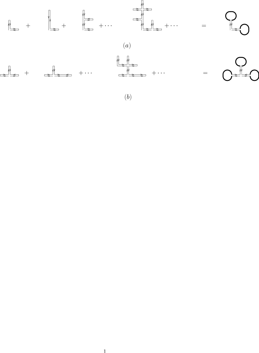
Figure 1: Sum of: (a) 2-trunk; and (b) 3-trunk trees

The set of all trees is now recovered by summing over all full n-trunk trees including the zeroth-order $n=0$ (no bottom-trunk), i.e. the bare propagator term. The resulting equation, depicted graphically in Fig.2, provides now a self-consistent equation for $G(x,x)$ in the large $N$ limit.

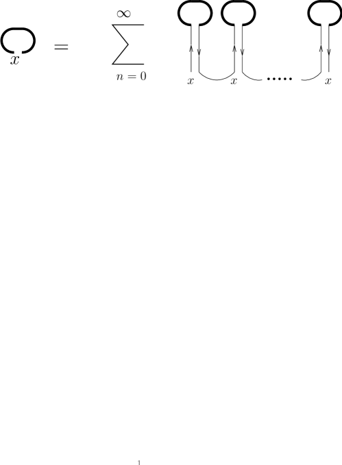
Figure 2: The self-consistent equation for the sum of trees attached to site $x$, i.e. $G(x,x)$

With constant (position-independent) source $K$, translation invariance implies that $G(x,x)$ is in fact $x$-independent. Using the explicit expressions (5), and bare propagator given by $\bar{K}^{-1}{\bf 1_{\scriptscriptstyle C}}$, the r.h.s. in this equation may be easily evaluated. One finds

$$G = \left[{\bf 1}_{\scriptscriptstyle C}+\sum_{n=1}^{\infty}\left[{(-1)\over 2}\,\bar{K}^{-1}\,\gamma^{\mu}G\gamma_{\mu}\right]^{n}\right]\bar{K}^{-1}$$ (8)

$$= \left[\bar{K}{\bf 1}_{\scriptscriptstyle C}+{1\over 2}\,\gamma^{\mu}G\gamma_{\mu}\right]^{-1}\,.$$ (9)

The hopping expansion which, in the large $N$ limit, gave (8) converges for sufficiently large $||K||$. The resumed expression (9), however, can be continued for all $K$. In particular, one is interested in possible solutions to (9) for $K\to 0$.

(9) was obtained by resummation of the (infinite) set of leading graphs in the large $N$ limit. An alternative approach is the direct construction of the corresponding effective action defined as the Legendre transform $\hat{\Gamma}(G)$ of the free-energy w.r.t. the source $K$. Since here we deal with composite, viz. bilinear fermion operators, this is the effective action for composite operators [8]. It is in fact quite straightforward to apply the general expression for the effective action given in [8] to the theory (3) in the strong coupling limit. Variation of the resulting effective action $\hat{\Gamma}(G)$ again yields (9), as expected. This is in fact a rather more efficient and elegant way of arriving at the result: only one 2-PI graph need be evaluated in the large $N$ limit.

We also note in passing that still another approach is that proposed in [6]. This approach, however, is mathematically inherently ambiguous and care must be exercised in applying it. If this is done it gives the same qualitative results but in a much lengthier and inefficient manner.

It is now easy to examine particular solutions of (9) that are picked out by appropriate choice of the source $K$. (We will not examine here the most general solution.) In all cases at large $||K||$ the solution reproduces, of course, the perturbative hopping expansion solution. We are, however, interested in the vanishing-source limit. In the case of scalar source, the solution is $G=g_{S}(K){\bf 1_{\scriptscriptstyle D}}{\bf 1_{\scriptscriptstyle C}}$, and one finds $g_{S}(0)=\sqrt{{2\over d}}$. For the scalar condensate one thus gets

$$\Big{\langle}\bar{\psi}(x)\psi(x)\Big{\rangle}=-NS\sqrt{{2\over d}}\,,$$ (10)

where $S={\rm tr}{\bf 1_{\scriptscriptstyle D}}$ is the number of spinor components. This reproduces the result in [5]. For vector or axial vector source $K=k(\Gamma\cdot n){\bf 1_{\scriptscriptstyle C}}$, the solution is of the form $G=g(k)(\Gamma\cdot n)^{-1}{\bf 1_{\scriptscriptstyle C}}$, where $\Gamma^{\mu}$ stands for either $\Gamma_{V}^{\mu}$ or $\Gamma_{A}^{\mu}$. (Note that in either case one has $(\Gamma\cdot n)^{-1}=(\Gamma\cdot n)$.) One now finds $g_{V}(0)=i\sqrt{2/(d-2)}$ whereas $g_{A}(0)=\sqrt{2/(d-2)}$. For the axial vector condensate one thus gets

$$\Big{\langle}\bar{\psi}(x)\,i\gamma^{5}\gamma^{\mu}\,\psi(x)\Big{\rangle}=-NS\sqrt{{2\over(d-2)}}\,n^{\mu}\,.$$ (11)

In the vector case, however, the resulting expectation is imaginary. Indeed, the solution turns complex for small source $K$. This would seem to indicate that no vector condensate actually forms. But this does not mean that other condensates induced in the presence of a vector source do not survive as the source is turned of. Consider the operator $\bar{\psi}(x)\gamma^{\mu}\sigma_{\kappa\lambda}\psi(x)$, where $\sigma_{\kappa\lambda}={i\over 2}[\gamma_{\kappa},\gamma_{\lambda}]$. This condensate, which is of interest for LSB-induced gravity theories, is also induced in the presence of a vector source. In this case in the vanishing-source limit one gets

$$\Big{\langle}\bar{\psi}(x)\gamma^{\mu}\sigma_{\kappa\lambda}\psi(x)\Big{\rangle}=NS\sqrt{{2\over(d-2)}}\;[\,g^{\mu}_{\kappa}n_{\lambda}-g^{\mu}_{\lambda}n_{\kappa}\,]\,.$$ (12)

Other chiral or Lorentz symmetry-breaking condensates involving more complicated operators such as lattice nearest-neighbor (continuum derivative) couplings may also be induced. The (gauge invariant) operator

$$O_{\nu\mu}(x)\equiv\bar{\psi}(x)\gamma_{\nu}U_{\mu}(x)\psi(x+\hat{\mu})-\bar{\psi}(x)\gamma_{\nu}U^{\dagger}_{\mu}(x-\hat{\mu})\psi(x-\hat{\mu})\,,$$ (13)

in particular, is of special interest. In its continuum limit it corresponds to the tensor operator $\bar{\psi}(x)\gamma^{\nu}\partial_{\mu}\psi(x)$, for which a non-vanishing condensate is a natural starting point for a theory of the graviton as a Goldstone boson [3]. In the presence of a vector (or axial vector) source (13) acquires a non-zero expectation. The full expectation is obtained by attaching the full set of trees, i.e. full propagators $G$ at the sites $x$ and $x+\hat{\mu}$ giving the graph shown in Fig.3. This is easily evaluated and in the limit of vanishing source yields

$$\Big{\langle}O_{\nu\mu}\Big{\rangle}=-{1\over(d-2)}NS\left[2n_{\nu}n_{\mu}-g_{\nu\mu}\right]\,.$$ (14)

(14) is a non-vanishing tensorial condensate not proportional to $g_{\nu\mu}$, i.e. an $SO(4)$-breaking (Lorentz-breaking) condensate. (A tensorial condensate proportional to the metric tensor is not Lorentz-breaking.) Different patterns of breaking, partial or complete, can be obtained by including fermions $\psi^{i}(x)$ of different flavor $i$ coupled to vector sources of different orientation $n_{i}^{\mu}$. If $N_{F}$ flavors are present (14) becomes

$$\Big{\langle}O_{\nu\mu}\Big{\rangle}={1\over 2}NN_{F}S\left[\,g_{\nu\mu}-{2\over N_{F}}\sum_{i}n^{i}_{\nu}n^{i}_{\mu}\right]\,.$$ (15)

The strongly coupled lattice model considered here provides in fact an explicit realization of the scenario envisioned in [3]. One may, for contrast, also consider the effect of the scalar condensate on (13). Repeating the calculation with a scalar source replacing the vector source one now gets that $\Big{\langle}O_{\nu\mu}\Big{\rangle}$ is proportional to $g_{\nu\mu}$. Thus, as expected, no Lorentz symmetry breaking is induced in this case.

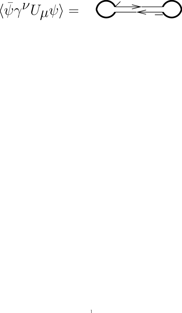
Figure 3: Graph for the expectation after attaching full trees; the short lines denote the different directions of the $\gamma^{\nu}$, $\gamma^{\mu}$ factors in it.

When internal (global) symmetry groups are present, a further possibility arises, i.e. condensate formation that ’locks’ space-time and internal symmetries. This possibility can be equally well explored within our strong coupling lattice gauge models.

The most straightforward example is provided by taking the internal symmetry to be a copy of the (Euclidean) space-time symmetry, i.e. an internal $SO(d)$ group with the fermions transforming as Dirac spinors under it. Denoting the gamma matrices acting on the internal space by $\gamma^{m}$, consider the operator $\bar{\psi}(x)\gamma^{n}\,(i\gamma_{5}\gamma_{\nu})\psi(x)$ involving an internal vector and an external axial vector. Non-vanishing vev’s of such fermion bilinears can lead to locking between the corresponding groups. To compute such a vev we again first introduce appropriate sources. Different fermion flavors can be coupled to different sources. In $d=4$ take the number of flavors to be (a multiple of) four coupled to corresponding sources along the elements $n_{(i)}^{\mu}$ and $n_{(i)}^{m}$, $i=1,\ldots,4$, of an orthonormal tetrad set in external and internal space, respectively. Proceeding as before, either by tree resummation, or, more efficiently, by direct construction of the effective action, one now, in the limit of vanishing sources, obtains the result

$$\Big{\langle}\bar{\psi}(x)\gamma^{n}\,(i\gamma_{5}\gamma_{\nu})\psi(x)\Big{\rangle}=-NS^{2}\sum_{i}n_{(i)}^{n}n_{(i)\,\nu}=-NS^{2}\delta^{n}_{\nu}\,.$$ (16)

(16) represents complete locking of the internal and external symmetry, i.e. breaking to the diagonal $SO(4)$ subgroup of the original symmetry: $SO(4)\times SO(4)_{I}\to SO(4)_{D}$. The condensate remains invariant only under simultaneous equal internal and external rotations.

The obvious question arises: how can such locking work in Minkowski space? There appear to be two possible choices. One choice is the standard Wick rotation where the external group gets decompactified to $SO(3,1)$ whereas the internal group remains compact. The condensate (16) is now invariant only under simultaneous $SO(3)$ (spatial) rotations, i.e. $SO(3,1)\times SO(4)_{I}\to SO(3)_{D}$. The second possibility is to define the passage to Minkowski space to also involve a ‘Wick rotation’ of the internal group decompactifying it. Full locking then is preserved, i..e (16) remains invariant under $SO(3,1)_{D}$. The obvious difficulty now is that an internal non-compact group, such as $SO(3,1)$, possesses only non-unitary finite-dimensional representations. This, of course, leads in general to unitarity violation. The only way out is to take the fermions to transform under a unitary, i.e. an infinite dimensional representation of the internal non-compact group. For an internal group the usual formalism applies whether one uses finite or infinite dimensional unitary representations. The new feature implied by the use of an infinite dimensional representation is the infinite number of components associated with the internal group index. This locking mechanism may offer a novel approach to a quantum gravity theory. At any rate, it would be interesting to work out the effective field theory for it at low energies.

This research was partially supported by NSF-PHY-0852438.

References

- [1] J.D. Bjorken, Ann. Phys. (N.Y.) 24 (1963) 174; hep-th/0111196.
- [2] P.R. Phillips, Phys. Rev. 146 (1966) 966; H.C. Ohanian, Phys. Rev. 184 (1969) 1305.
- [3] P. Kraus and E.T. Tomboulis, Phys. Rev. D 66 (2002) 045015.
- [4] S.M. Carroll, H. Tam and I.K. Wehus, Phys. Rev. D 80 (20009) 025020; Z. Berezhiani and O.V. Kancheli, arXiv:0808.3181v1 [hep-th]; A. Kostelecky and R. Potting, Phys. Rev. D 79 (2009) 065018.
- [5] J-M Blairon, R. Brout, F. Englert and J. Greensite, Nucl. Phys. B 180[FS2] (1981) 439.
- [6] N. Kawamoto and J. Smit, Nucl. Phys. B 192 (1981) 100; H. Kluberg-Stern, A. Morel, O. Napoly and B. Peterson, Nucl. Phys. B 190 [FS3] (1981) 504.
- [7] H.J. Rothe, Lattice Gauge Theories, World Scientific, Singapore, 3rd ed., 2005; I.O. Stamatescu, Phys. Rev. D25 (1982) 1130.
- [8] J.M. Cornwell, R. Jackiw and E.T. Tomboulis, Phys. Rev. D 10(1974) 2428.