Non-perturbative predictions for cold atom Bose gases with tunable interactions

Abstract

We derive a theoretical description for dilute Bose gases as a loop expansion in terms of composite-field propagators by rewriting the Lagrangian in terms of auxiliary fields related to the normal and anomalous densities. We demonstrate that already in leading order this non-perturbative approach describes a large interval of coupling-constant values, satisfies Goldstone’s theorem, yields a Bose-Einstein transition that is second-order, and is consistent with the critical temperature predicted in the weak-coupling limit by the next-to-leading order large-N expansion.

Nearly a century after the first observation of the lambda transition in liquid heliumKamerling (1911), a quantitative, first-principles description of strongly-correlated bosons remains a challenge. After the transition was recognized as the onset of superfluidityKapitza (1938); *r:Allen:1938vn, the connection with Bose-Einstein condensation (BEC) was proposedLondon (1938); *r:London:1938zr, but it was Bogoliubov’s workBogoliubov (1947) pointing out that the dispersion of the elementary BEC excitations satisfy the Landau criterion for superfluidityLandau (1941) that motivated weakly-interacting BEC studies to investigate superfluid properties. In weakly-interacting systems, the many-body properties do not depend on the shape of the interaction potential, but only on the $s$-wave scattering length, $a_{0}$, and the boson fluid acts as point-like interacting particlesLee et al. (1957).

Unlike liquid helium, cold atoms remain point-like even when the scattering length is tuned near a Feshbach resonance. Then, strongly-correlated cold atom bosons offer the exciting prospect of studying point-like strongly interacting bosons, possibly in the universal regime where the scattering length greatly exceeds the inter-particle distance and the latter becomes the only relevant length scaleShin et al. (2007). This hope appeared thwarted when it was shown that the three-body loss rate in cold atom traps scales as $a_{0}^{4}$ near a Feshbach resonanceFedichev et al. (1996); *r:Esry:1991ij. In accordance, the universal regime was reached only in ultra-cold fermionic gasesHo (2004); *r:Blume:2007tg, where the three-body loss is reduced by virtue of the Pauli exclusion principle. However, the recent observation that three-body losses are strongly suppressed in optical lattices when the average number of bosons per site is two or lessDaley et al. (2009), rekindles the prospect of studying medium and strongly-correlated cold atom bosons. Novel cold-atom trap technologies that produce stable, flat potentials bound by a sharp edgeHenderson et al. (2006); *r:Henderson:2009dz, suggest the study of finite-temperature properties such as the BEC transition temperature $T_{c}$ and the superfluid to normal fluid ratio and depletion, at fixed density, $\rho$.

At finite temperature, the description of BEC’s remains a challenge even in the weakly-interacting regime. Standard approximations such as the Hartree-Fock-Bogoliubov and the Popov schemes, generally fall within the Hohenberg and Martin classificationHohenberg and Martin (1965) of conserving and gapless approximations, which implies that they either violate Goldstone’s theorem or general conservation lawsGriffin (1996). These approximations generally predict the BEC transition to be a first-order transition, whereas we expect the transition to be second orderAndersen (2004).

In this paper, we present a new theoretical framework that describes a large interval of $\rho^{1/3}a_{0}$-values, satisfies Goldstone’s theorem and yields a Bose-Einstein transition that is second-order, while also predicting reasonable values for the depletion. Furthermore, this framework can predict all experimentally relevant quantities within the same calculation, determining fully consistently quantities such as $T_{c}$, the collective mode frequenciesref and the compressibility (which characterizes the density profile in a shallow trapref ). In contrast with other resummation schemes, such as the large-$N$ expansionBaym et al. (2000) or functional renormalization techiquesFloerchinger and Wetterich (2008), here we treat the normal and anomalous densities on equal footing.

In our approach, we generate a one-parameter family of equivalent Lagrangians. We choose this parameter to reproduce the one-loop result at mean-field level in the weakly-interacting limit. Thus, we identify the optimal auxiliary-field Lagrangian for the purpose of a systematic non-perturbative expansion. Then, the critical temperature variation in leading order is the same as the one found in the next-to-leading order large-$N$ expansion.

In dilute bosonic gas systems, the classical action is given by $S[\,\phi,\phi^{\ast}\,]=\int\!\mathrm{d}x\>\mathcal{L}[\,\phi,\phi^{\ast}\,]$, with $\mathrm{d}x\equiv\mathrm{d}t\,\mathrm{d}^{3}x$ and the Lagrangian density

$$\mathcal{L}[\,\phi,\phi^{\ast}\,]=\frac{i\hbar}{2}\,[\,\phi^{\ast}(x)\,(\partial_{t}\,\phi(x))-(\partial_{t}\,\phi^{\ast}(x))\,\phi(x)\,]$$

$${}-\phi^{\ast}(x)\,\Bigl{\{}\,-\frac{\hbar^{2}\nabla^{2}}{2m}-\mu\,\Bigr{\}}\,\phi(x)-\frac{\lambda}{2}\,|\,\phi(x)|^{4}\>.$$ (1)

Here, $\mu$ is the chemical potential and the coupling is $\lambda=4\pi\hbar^{2}\,a_{0}/m$. To account for the contributions of the normal and anomalous densities, we use the Hubbard-Stratonovitch transformationHubbard (1959); *r:Stratonovich:1958vn to introduce the real and complex auxiliary fields (AF), $\chi(x)$ and $A(x)$. We add to Eq. (1) the AF Lagrangian densityBender et al. (1977); Coleman et al. (1974); *r:Root:1974qf

$$\mathcal{L}_{\text{aux}}[\phi,\phi^{\ast},\chi,A,A^{\ast}]=\frac{1}{2\lambda}\,\bigl{[}\,\chi(x)-\lambda\,\cosh\theta\,|\phi(x)|^{2}\,\bigr{]}^{2}$$

$$\qquad{}-\frac{1}{2\lambda}\,\bigl{|}\,A(x)-\lambda\,\sinh\theta\,\phi^{2}(x)\,\bigr{|}^{2}\>,$$ (2)

where $\theta$ is the mixing parameter between the normal and anomalous densities, $\chi(x)$ and $A(x)$. The usual large-N approximationColeman et al. (1974); *r:Root:1974qf is obtained when $\theta=0$. Then, the action becomes

$$S[\Phi,J]=S[\phi_{a},\chi,A,A^{\ast},j_{a},s,S]$$ (3)

$$\quad=-\frac{1}{2}\,\iint\mathrm{d}x\,\mathrm{d}x^{\prime}\,\phi_{a}(x)\,G^{-1}{}^{a}{}_{b}[\chi,A](x,x^{\prime})\,\phi^{b}(x^{\prime})$$

$$\qquad{}+\int\mathrm{d}x\,\bigl{\{}\,\bigl{[}\,\chi^{2}(x)-|A(x)|^{2}\,\bigr{]}/(2\lambda)-s(x)\chi(x)$$

$$+S^{\ast}(x)A(x)+S(x)A^{\ast}(x)+j^{\ast}(x)\phi(x)+j(x)\phi^{\ast}(x)\,\bigr{\}}\>,$$

with

$$G^{-1}{}^{a}{}_{b}[\chi,A]=\bigl{\{}\,G^{-1}_{0}{}^{a}{}_{b}+V^{a}{}_{b}[\chi,A](x)\,\bigr{\}}\delta(x,x^{\prime})\,\>,$$

$$G^{-1}_{0}{}^{a}{}_{b}=\begin{pmatrix}h_{0}&0\\[3.0pt] 0&h_{0}^{\ast}\end{pmatrix}\>,\quad h_{0}=-\frac{\hbar^{2}\nabla^{2}}{2m}-i\hbar\frac{\partial}{\partial t}-\mu\>,$$ (4)

$$V^{a}{}_{b}[\chi,A](x)=\begin{pmatrix}\chi(x)\cosh\theta&-A(x)\sinh\theta\\ -A^{\ast}(x)\sinh\theta&\chi(x)\cosh\theta\end{pmatrix}\>.$$

Here, we introduced a two-component notation with $\phi^{a}(x)=\{\,\phi(x),\phi^{\ast}(x)\,\}$ for $a=1,2$. $\Phi(x)$ and $J(x)$ signify the five-component fields and currents. The generating functional for connected graphs is

$$Z[J]=e^{iW[J]/\hbar}=\mathcal{N}\int\mathrm{D}\Phi\>e^{iS[\Phi;J]/\hbar}\>,$$

with $S[\Phi;J]$ given by Eq. (3). Performing the path integral over the fields $\phi_{a}$, we obtain the effective action

$$\epsilon\,S_{\text{eff}}[\chi;J,\epsilon]=\frac{1}{2}\iint\mathrm{d}x\,\mathrm{d}x^{\prime}\,j_{a}(x)\,G[\chi]^{a}{}_{b}(x,x^{\prime})\,j^{a}(x)$$

$${}+\int\mathrm{d}x\,\Bigl{\{}\,\frac{\chi_{i}(x)\,\chi^{i}(x)}{2\lambda}-S_{i}(x)\,\chi^{i}(x)-\frac{\hbar}{2i}\text{Tr}\,\ln[\,G^{-1}\,]\,\Bigr{\}}\>,$$

where $\chi^{i}(x)=\bigl{\{}\chi(x),A(x)/\sqrt{2},A^{\ast}(x)/\sqrt{2}\bigr{\}},\>S^{i}(x)=\bigl{\{}s(x),S(x)/\sqrt{2},S^{\ast}(x)/\sqrt{2}\bigr{\}}$. The small parameter $\epsilon$ allows us to perform the remaining path integral over $\chi^{i}$ using the stationary-phase approximation. As shown in Ref.Bender et al., 1977, $\epsilon$ counts loops in the AF propagator in analogy with $\hbar$, and provides the loop expansion of the effective action in terms of $\chi$ propagators. Next, we expand the effective action about the stationary points, $\chi_{0}^{i}(x)$, defined by $\delta S_{\text{eff}}[\chi;j]/\delta\chi_{i}(x)=0$. Hence, we obtain

$$\frac{\chi_{0}(x)}{\lambda} =\bigl{\{}\,|\phi_{0}(x)|^{2}+\frac{\hbar}{2i}\,\mathrm{Tr}[\,G(x,x)\,]\,\bigr{\}}\,\cosh\theta+s(x)\>,$$

$$\frac{A_{0}(x)}{\lambda} =\bigl{\{}\,\phi^{2}_{0}(x)+\frac{\hbar}{i}\,G^{2}{}_{1}(x,x)\,\bigr{\}}\,\sinh\theta+S(x)\>,$$

where we introduced the notations

$$\phi^{a}_{0}[\chi_{0}](x)=\int\mathrm{d}x^{\prime}\,G[\chi_{0}]^{a}{}_{b}(x,x^{\prime})\,j^{b}(x^{\prime})\>.$$

We emphasize that both $\chi_{0}$ and $A_{0}$ include self-consistent fluctuations. Expanding the effective action about the stationary point, we write

$$S_{\text{eff}}[\chi;J]=S_{\text{eff}}[\chi_{0};J]+\frac{1}{2}\iint\mathrm{d}^{4}x\,\mathrm{d}^{4}x^{\prime}\,D_{ij}^{-1}[\chi_{0}](x,x^{\prime})$$

$$\qquad{}\times[\chi^{i}(x)-\chi^{i}_{0}(x)]\,[\chi^{j}(x^{\prime})-\chi^{j}_{0}(x^{\prime})]+\dotsb\>,$$ (5)

where $D_{ij}^{-1}(x,x^{\prime})$ is given by the second-order derivatives,

$$D_{ij}^{-1}[\chi_{0}](x,x^{\prime})=\frac{\delta^{2}\,S_{\text{eff}}[\chi^{a}]}{\delta\chi^{i}(x)\,\delta\chi^{j}(x^{\prime})}\,\bigg{|}_{\chi_{0}}\>,$$

evaluated at the stationary points. By keeping the gaussian fluctuations and Legendre transforming, the one-particle irreducible (1-PI) graphs generating functional

$$\Gamma[\Phi]=\int\mathrm{d}x\,j_{\alpha}(x)\,\phi^{\alpha}(x)-W[J]$$ (6)

$$=\frac{1}{2}\iint\mathrm{d}x\,\mathrm{d}x^{\prime}\,\phi_{a}(x)\,G^{-1}[\chi]^{a}{}_{b}(x,x^{\prime})\,\phi^{b}(x^{\prime})$$

$$\quad{}-\int\mathrm{d}x\,\Bigl{\{}\,\frac{\chi_{i}(x)\,\chi^{i}(x)}{2\lambda}-\frac{\hbar}{2i}\text{Tr}\bigl{\{}\,\ln[\,G^{-1}[\chi](x,x)\,]\,\bigr{\}}$$

$$\qquad\qquad\qquad{}-\frac{\hbar\,\epsilon}{2i}\,\text{Tr}\,\ln[\,D_{ii}^{-1}[\Phi](x,x)\,]\,\Bigr{\}}+\dotsb\>,$$

is the negative of the classical action plus self-consistent one-loop corrections in the $\phi_{a}$ and $\chi_{i}$ propagators.

To leading order in the AF loop expansion (LOAF), one sets $\epsilon=0$ in the right-hand-side of (6). The static part of the effective action per unit volume is

$$V_{\text{eff}}[\Phi] =(\chi\cosh\theta-\mu\,)\,|\phi|^{2}-\frac{1}{2}\,(A^{\ast}\,\phi^{2}+A\,\phi^{\ast\,2})\sinh\theta$$

$$\qquad{}-\frac{\chi^{2}-|A|^{2}}{2\lambda}+\frac{\hbar}{2i}\text{Tr}\bigl{\{}\,\ln[\,G^{-1}[\chi]\,]\,\bigr{\}}\>.$$ (7)

Translating (7) to the imaginary time formalism, we find

$$\frac{\hbar}{2i}\text{Tr}\,\ln[\,G^{-1}[\chi]\,]=\int\frac{\mathrm{d}^{3}k}{(2\pi)^{3}}\,\Bigl{\{}\,\frac{\omega_{k}}{2}+\frac{1}{\beta}\,\ln[\,1-e^{-\beta\omega_{k}}\,]\,\Bigr{\}}\>,$$

where $\omega_{k}^{2}=(\epsilon_{k}+\chi\,\cosh\theta-\mu)^{2}-|A|^{2}\sinh^{2}\theta$ and $\epsilon_{k}=k^{2}/(2m)$. At the minimum, we have

$$\frac{\delta V_{\text{eff}}[\Phi]}{\delta\phi^{\ast}}\Bigl{|}_{\phi_{0}}=(\chi\cosh\theta-\mu)\,\phi_{0}-A\,\sinh\theta\,\phi_{0}^{\ast}=0\>.$$ (8)

Using the $U(1)$ gauge symmetry, we choose $\phi_{0}$ to be real. Then, $A$ is real and the dispersion, $\omega_{k}^{2}=\epsilon_{k}(\epsilon_{k}+2A\sinh\theta)$, represents the Goldstone theorem. Next, we set $\sinh\theta=1$, such that $\omega_{k}$ reduces to the Bogoliubov dispersion, $\omega_{k}=\sqrt{\epsilon_{k}(\epsilon_{k}+2\lambda\,\phi_{0}^{2})}$, in the limit of vanishing quantum fluctuations in the anomalous density. We note that the leading-order (LO) in the large-N expansion corresponds to $\theta=0$. This leads to the noninteracting (NI) dispersion, $\omega_{k}=\epsilon_{k}$, and we conclude that the large-N expansion is not a suitable starting point, because it is incompatible with the Bogoliubov spectrum.

Using standard regularization techniquesPapenbrock and Bertsch (1999), the renormalized effective potential is written as

$$V_{\text{eff}}[\Phi]=\chi^{\prime}|\phi|^{2}-\frac{1}{2}\bigl{(}A^{\ast}\phi^{2}+A\phi^{\ast\,2}\bigr{)}-\frac{(\chi^{\prime}+\mu)^{2}}{4\lambda}+\frac{|A|^{2}}{2\lambda}$$

$$+\!\!\int\!\!\frac{\mathrm{d}^{3}k}{(2\pi)^{3}}\Bigl{[}\frac{1}{2}\Bigl{(}\omega_{k}-\epsilon_{k}-\chi^{\prime}+\frac{|A|^{2}}{2\epsilon_{k}}\Bigr{)}\!+\frac{1}{\beta}\ln(1-e^{-\beta\omega_{k}})\Bigr{]},$$

where $\chi^{\prime}\!=\!\sqrt{2}\chi-\mu$ and $\omega_{k}^{2}=\!(\epsilon_{k}+\chi^{\prime}+|A|)(\epsilon_{k}+\chi^{\prime}-|A|)$. The gap equations, obtained from $\delta V_{\text{eff}}[\Phi]/\delta\chi^{i}=0$, are

$$\frac{A}{\lambda} =\phi^{2}+A\int\frac{\mathrm{d}^{3}k}{(2\pi)^{3}}\,\Bigl{\{}\frac{1+2n(\omega_{k})}{2\omega_{k}}-\frac{1}{2\epsilon_{k}}\Bigr{\}}\>,$$ (9)

$$\frac{\chi^{\prime}+\mu}{2\lambda} =|\phi|^{2}+\int\frac{\mathrm{d}^{3}k}{(2\pi)^{3}}\,\Bigl{\{}\frac{\epsilon_{k}+\chi^{\prime}}{2\omega_{k}}[1+2n(\omega_{k})]-\frac{1}{2}\Bigr{\}}\>,$$

where $n(\omega_{k})=[\exp(\omega_{k}/k_{B}T)-1]^{-1}$ is the Bose-Einstein particle distribution. At the minimum of the effective potential we have, $(\chi^{\prime}_{0}-A_{0})\,\phi_{0}=0$, see Eq. (8), and we replace $\mu$ by the physical density using $\rho=-\partial V_{\text{eff}}[\Phi_{0}]/\partial\mu=(\chi^{\prime}_{0}+\mu)/(2\lambda)$. The density is used to rescale Eqs. (9), and the ensuing phase diagram problem depends only on the dimensionless parameter, $\rho^{1/3}a_{0}$, and the coupling constant becomes $\lambda=8\pi\,\rho^{1/3}a_{0}$. In the broken symmetry phase, we have $\chi^{\prime}_{0}=A_{0}$ and the dispersion relation, $\omega_{k}^{2}=\epsilon_{k}(\epsilon_{k}+2\chi^{\prime}_{0})$. The condensate density is denoted by $\rho_{0}=\phi_{0}^{2}$. At weak coupling and $T=0$, our results coincide with the Bogoliubov (one-loop) approximationAndersen (2004), $\mu=8\pi\rho a_{0}\bigl{[}1+(32/3)\sqrt{\rho a_{0}^{3}/\pi}\,\bigr{]}$.

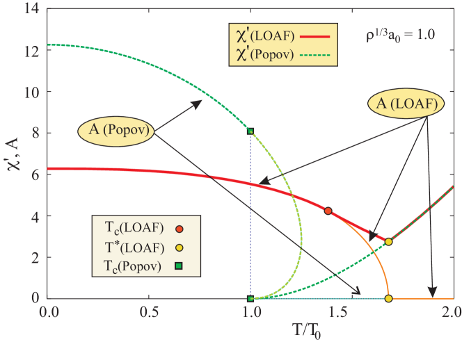
Figure 1: (Color online) Normal density, $\chi^{\prime}$, and anomalous density, $A$, from the LOAF and PA approximations, for $\rho^{1/3}a_{0}=1$. $T_{c}$ and $T^{\star}$ indicate vanishing condensate density, $\rho_{0}$, and anomalous density, $A$, respectively. PA leads to a first-order phase transition, whereas LOAF predicts a second-order phase transition. We have that $T_{c}=T^{\star}$ in the PA, but not in LOAF. In LOAF $\chi^{\prime}$ and $A$ are equal until $T_{c}$.

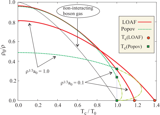
Figure 2: (Color online) Temperature dependence of the condensate fractions from LOAF and PA, compared with the NI result, for $\rho^{1/3}a_{0}=0.1$ and $\rho^{1/3}a_{0}=1$. Because at $T_{c}$ the PA and NI dispersion relations are the same, PA does not change $T_{c}$ relative to the NI case. LOAF increases $T_{c}$.

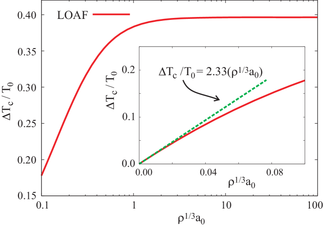
Figure 3: (Color online) Relative change in $T_{c}$ with respect to NI, as predicted by LOAF as a function of $\rho^{1/3}a_{0}$. The inset shows that in the weak-coupling regime, LOAF produces the same slope as the next-to-leading order large-N expansionBaym et al. (2000).

We compare the LOAF results with the predictions of the Popov bosonic approximation (PA)Popov (1987). PA is generally recognized as an accurate theoretical description of experimental data in weakly-coupled dilute trapped Bose gasesDalfovo et al. (1999), as long as the densities of the condensed and noncondensed atoms are comparable with each other. Unfortunately, PA produces an artificial first-order phase transition at $T_{c}$. Formally, PA is obtained from Eq. (9) by setting $A_{0}=\chi_{0}^{\prime}=\lambda\rho_{0}$ and neglecting the quantum fluctuations in the anomalous density. With this substitution, the PA dispersion relation reads $\omega_{k}^{2}=\epsilon_{k}(\epsilon_{k}+2\lambda\rho_{0})$.

In Fig. 1 we depict the temperature dependence of the normal density $\chi^{\prime}$, and anomalous density, $A$, at constant $\rho^{1/3}a_{0}$, as derived using the LOAF and PA approximations. For illustrative purposes, we set $\rho^{1/3}a_{0}=1$ and the temperature is scaled by its NI critical value, $T_{0}=(2\pi\hbar^{2}/m)[\rho/\zeta(3/2)]^{2/3}$, where $\zeta(x)$ is the Riemann zeta function. We identify two special temperatures, at $T_{c}$ where the condensate density vanishes, and at $T^{\star}$ where the anomalous density, $A$, vanishes. These temperatures are the same in the PA formalism, but they are different in LOAF. The existence of a temperature range, $T_{c}<T<T^{\star}$, for which the anomalous density, $A$, is nonzero despite a zero condensate fraction, $\phi$, is a fundamental prediction of LOAF. In this temperature range, the dispersion relation is expected to depart from the quadratic form predicted by the Popov approximation for $T>T_{c}$. Above $T_{c}$ the solution of the PA equations becomes multivalued, indicating that the system undergoes a first-order phase transition at $T_{c}$. In contrast, LOAF predicts a second-order transition.

The temperature dependence of the condensate fraction, $\rho_{0}/\rho$, is depicted in Fig. 2 for two constant values of the dimensionless parameter $\rho^{1/3}a_{0}$, together with the NI result, $\rho_{0}/\rho=1-(T/T_{0})^{3/2}$. Again, we observe that LOAF exhibits the correct second-order BEC phase transition behavior. Moreover, PA does not change $T_{c}$ relative to the NI case, because in the PA case we have $T_{c}=T^{\star}$ and the PA and NI dispersion relations are the same at $T_{c}$. The LOAF approximation predicts an increase of $T_{c}$ compared with the NI case.

As illustrated in Fig. 2, the LOAF and PA predictions may differ greatly even for temperatures, $T\ll T_{c}$. These differences are enhanced by a strengthening of the interaction between particles in the Bose gas (a larger value of $\rho^{1/3}a_{0}$ indicates stronger coupling). The leading-order AF formalism produces a more realistic set of observables away from the weak-coupling limit because of its non-perturbative character. In contrast, PA is appropriate only in the case of a weakly-interacting gas of bosons. The former is made explicit by studying the LOAF prediction for the relative change in $T_{c}$ with respect to $T_{0}$, as a function of $\rho^{1/3}a_{0}$. The inset in Fig. 3 demonstrates that in the weak-coupling regime, $\rho^{1/3}a_{0}\ll 1$, LOAF produces the same slope of the linear departure derived by Baym et al.Baym et al. (2000) using the large-N expansion, but at next-to-leading order. The LOAF corrections to the critical temperature are due to the inclusion of self-consistent fluctuations effects in the mean-field $\chi^{\prime}$ and $A$ densities. A summary of $\Delta T_{c}/T_{0}$ theoretical predictions is found in Ref.Andersen, 2004. For $\rho^{1/3}a_{0}\gg 1$, LOAF predicts that $\Delta T_{c}/T_{0}\rightarrow 0.396$ when the system approaches the unitarity limit. Despite that most current experiments probe only the $\rho^{1/3}a_{0}\ll 1$ regime, future experimentsHenderson et al. (2006); *r:Henderson:2009dz may access the medium-to-strongly interacting regime, and verify this non-perturbative prediction.

One can systematically improve upon the LOAF approximation by calculating the 1-PI action order-by-order in $\epsilon$. The broken $U(1)$ symmetry Ward identities guarantee Goldstone’s theorem order by order in $\epsilon$ Bender et al. (1977). For time-dependent problems, however, this expansion is secularMihaila et al. (2001), and a further resummation is required. The latter is performed using the two-particle irreducible (2-PI) formalismBaym (1962); *r:CJT. A practical implementation of this approach is the bare-vertex approximation (BVA)Blagoev et al. (2001). The BVA is an energy-momentum and particle-number conserving truncation of the Schwinger-Dyson infinite hierarchy of equations obtained by ignoring the derivatives of the self-energy, similarly to the Migdal’s theoremMigdal (1958) approach in condensed matter physics. The BVA proved effective in the case of classical and quantum $\lambda\phi^{4}$ field theory problemsCooper et al. (2003); *r:CDM02ii; *r:Mihaila:2003ys and can be applied to the BEC case.

To summarize, in this paper we introduce a new non-perturbative resummation formulation for the BEC problem. At mean-field level, this approach meets three important criteria for a satisfactory mean-field theory for weakly-interacting bosonsAndersen (2004): i) the excitation spectrum is gapless (to preserve Goldstone’s theorem), ii) LOAF reduces to the known results from Bogoliubov theory at $T=0$ and weak coupling, and iii) predicts a second-order BEC phase transition. The latter suggests that a AF formulation of the Lagrangian for systems of cold fermionic atoms may also impact the study of the BEC to BCS crossover in dilute fermionic atom systemsLevin et al. (2010).

Work performed in part under the auspices of the U.S. Department of Energy. The authors would like to thank E. Mottola and P.B. Littlewood for useful discussions.

References

- Kamerling (1911) O. H. Kamerling, Proc. Roy. Acad. Amsterdam, 13, 1903 (1911).
- Kapitza (1938) P. L. Kapitza, Nature, 141, 74 (1938).
- Allen and Misener (1938) J. F. Allen and A. D. Misener, Nature, 141, 75 (1938).
- London (1938) F. London, Nature, 141, 643 (1938a).
- London (1938) F. London, Phys. Rev., 54, 947 (1938b).
- Bogoliubov (1947) N. N. Bogoliubov, J. Phys. USSR, 11, 23 (1947).
- Landau (1941) L. D. Landau, J. Phys. USSR, 5, 71 (1941).
- Lee et al. (1957) T. D. Lee, K. Huang, and C. N. Yang, Phys. Rev., 106, 1135 (1957).
- Shin et al. (2007) Y. Shin, C. H. Schunck, A. Schirotzek, and W. Ketterle, Phys. Rev. Lett., 99, 090403 (2007).
- Fedichev et al. (1996) P. O. Fedichev, M. W. Reynolds, and G. V. Shlyapnikov, Phys. Rev. Lett., 77, 2921 (1996).
- Esry et al. (1999) B. D. Esry, C. H. Greene, and J. P. Burke, Phys. Rev. Lett., 83, 1751 (1999).
- Ho (2004) T. L. Ho, Phys. Rev. Lett., 92, 090402 (2004).
- Blume et al. (2007) D. Blume, J. von Stecher, and C. H. Greene, Phys. Rev. Lett., 99, 233201 (2007).
- Daley et al. (2009) A. J. Daley, J. M. Taylor, S. Diehl, M. Baranov, and P. Zoller, Phys. Rev. Lett., 102, 040402 (2009).
- Henderson et al. (2006) K. Henderson, H. Kelkar, T. C. Lee, B. Gutirez-Medina, and M. G. Raizen, Europhys. Lett., 75, 392 (2006).
- Henderson et al. (2009) K. Henderson, C. Ryu, C. MacCormic, and M. Boshier, New J. Phys., 11, 043030 (2009).
- Hohenberg and Martin (1965) P. C. Hohenberg and P. C. Martin, Ann. Phys., 34, 291 (1965).
- Griffin (1996) A. Griffin, Phys. Rev. B, 53, 9341 (1996).
- Andersen (2004) J. O. Andersen, Revs. Mod. Phys., 76, 599 (2004).
- (20) Collective modes have been measured in BECs, see J. M. Vogels, K. Xu, C. Raman, J. R. Abo-Shaeer, and W. Ketterle, Phys. Rev. Lett., 88, 060402 (2002), using a method that provides an experimental verification of the fact that the -momentum quasi-particle is a superposition of and waves. This mixing involves the anomalous density, so that the presence of an anomalous density above the BEC , as predicted by our theory, may be tested not only by measuring the frequency dispersion, but also by testing the mixing.
- (21) In the Thomas-Fermi approximation, the local BEC density, , in a trapping potential, , follows from the density-dependent chemical potential, . Taking the gradient of both sides, we find that the local trap force experienced by the bosons and the boson density gradient, , are proportional with a constant of proportionality equal to , related to the compressibility, . With the sensitive density profile measurement developed for fermion thermometry, experimentalists could, in principle, verify the compressibility calculation.
- Baym et al. (2000) G. Baym, J.-P. Blaizot, and J. Zinn-Justin, Europhys. Lett., 49, 150 (2000).
- Floerchinger and Wetterich (2008) S. Floerchinger and C. Wetterich, Phys. Rev. A, 77, 053603 (2008).
- Hubbard (1959) J. Hubbard, Phys. Rev. Lett., 3, 77 (1959).
- Stratonovich (1958) R. L. Stratonovich, Doklady, 2, 416 (1958).
- Bender et al. (1977) C. Bender, F. Cooper, and G. Guralnik, Ann. Phys., 109, 165 (1977).
- Coleman et al. (1974) S. Coleman, R. Jackiw, and H. D. Politzer, Phys. Rev. D, 10, 2491 (1974).
- Root (1974) R. Root, Phys. Rev. D, 10, 3322 (1974).
- Papenbrock and Bertsch (1999) T. Papenbrock and G. F. Bertsch, Phys. Rev. C, 59, 2052 (1999).
- Popov (1987) V. N. Popov, Functional integrals and collective excitations (Cambridge University Press, Cambridge, England, 1987).
- Dalfovo et al. (1999) F. Dalfovo, S. Giorgini, L. P. Pitaevskii, and S. Stringari, Rev. Mod. Phys., 71, 463 (1999).
- Mihaila et al. (2001) B. Mihaila, J. F. Dawson, and F. Cooper, Phys. Rev. D, 63, 096003 (2001).
- Baym (1962) G. Baym, Phys. Rev., 127, 1391 (1962).
- Cornwall et al. (1974) J. M. Cornwall, R. Jackiw, and E. Tomboulis, Phys. Rev. D, 10, 2428 (1974).
- Blagoev et al. (2001) K. B. Blagoev, F. Cooper, J. F. Dawson, and B. Mihaila, Phys. Rev. D, 64, 125003 (2001).
- Migdal (1958) A. B. Migdal, Sov. Phys. JETP, 7, 996 (1958).
- Cooper et al. (2003) F. Cooper, J. F. Dawson, and B. Mihaila, Phys. Rev. D, 67, 051901R (2003a).
- Cooper et al. (2003) F. Cooper, J. F. Dawson, and B. Mihaila, Phys. Rev. D, 67, 056003 (2003b).
- Mihaila (2003) B. Mihaila, Phys. Rev. D, 68, 036002 (2003).
- Levin et al. (2010) K. Levin, Q. J. Chen, C. C. Chien, and Y. He, Ann. Phys., 325, 233 (2010).