Simultaneous solution of Kompaneets equation and Radiative Transfer equation in the photon energy range 1 - 125 KeV

Abstract

Radiative transfer equation in plane parallel geometry and Kompaneets equation is solved simultaneously to obtain theoretical spectrum of 1-125 KeV photon energy range. Diffuse radiation field is calculated using time-independent radiative transfer equation in plane parallel geometry, which is developed using discrete space theory (DST) of radiative transfer in a homogeneous medium for different optical depths. We assumed free-free emission and absorption and emission due to electron gas to be operating in the medium. The three terms $n,n^{2}$ and $\displaystyle\bigg{(}{\frac{\partial n}{\partial x_{k}}}\bigg{)}$ where $n$ is photon phase density and $\displaystyle x_{k}=\bigg{(}{\frac{h\nu}{kT_{e}}}\bigg{)}$, in Kompaneets equation and those due to free-free emission are utilized to calculate the change in the photon phase density in a hot electron gas. Two types of incident radiation are considered: (1) isotropic radiation with the modified black body radiation $I^{MB}$ [1] and (2) anisotropic radiation which is angle dependent. The emergent radiation at $\tau=0$ and reflected radiation $\tau=\tau_{max}$ are calculated by using the diffuse radiation from the medium. The emergent and reflected radiation contain the free-free emission and emission from the hot electron gas. Kompaneets equation gives the changes in photon phase densities in different types of media. Although the initial spectrum is angle dependent, the Kompaneets equation gives a spectrum which is angle independent after several Compton scattering times.

1 Introduction

Compton and inverse Compton scattering play an important role in the processes of emission of X-ray spectrum which has been observed in many compact astronomical objects. Comptonization of X-rays has been dealt mostly through Fokker-Planck approximation (i.e, electron temperatures and photon frequencies are not high compared to the rest energy of the electron)[2][3] [4] [5] and others. Primary non thermal X-ray and $\gamma$-ray emission may reprocessed and end up in different energy band [6]. Several X-ray observations obtained by Ginga do not confirm the power law spectral shape [7], [8]. Spectral hardening have been noticed from Ginga satellite observations [7] [9] [10] and [11] of Seyfert galaxies and Cygx-1.

Analytical approximations of Compton reflection have been developed by [12], on the basis of the separation of spacial and energy transport in the transfer equation. This approach have the advantage of facility to explore the model parameters. Later, many authors [13] [14] [15] [16] and [17] to implement Monte Carlo methods to treat several aspects of Compton reflection models by taking more detail of the physics and geometry of the problem. Burigana [18] studied the reflection problem with semi analytical transfer equation and obtained the solution of the transfer equation. Angle dependent Compton reflection of X-rays and $\gamma$-rays has been studied by [19]. Studies on Compton reflection of X-rays and $\gamma$-rays by [12] [20] [21] and others in shaping the emergent X-ray and $\gamma$-ray spectra. Czerny & Elvis [22], Zdziarski et al [23] and Haardt & Marasachi [24] studied the inverse Compton scattering in producing the high energy photons in some of the compact sources in which low energy photons gain energy from hot electrons. The geometry and distribution of matter in these objects would make the process anisotropic [25] [6] [26]. Haardt & Marashi [24] and Haardt [27] studied this process in plane parallel geometry. Nishimura, Mitsadu & Itoh [28] studied the same problem but without angular dependence with isotropic scattering in the laboratory frame with $kT_{e}<$ 150 KeV.

The escape probability and the energy distribution of the single scattered photons are analytically calculated using Mellin integral transformations. Miyamoto [29] estimated the photon escape time distribution and effect of Comptonization on the spectrum. Katz [30] obtained space distribution of the photons and spectrum changes by solving Fokker-Planck equation from Shapiro et al [31]. The transfer of radiation estimated by using Monte-Carlo method [32]. Another characteristic of X-ray spectra is its variability over time. The time delay due to photon diffusion and the energy release and multiple scattering of X-ray photons with thermal electrons due to comptonization would change the nature of the emergent X-ray spectra. If $kT_{e}>h\nu$ then the photon gain energy and if $kT_{e}<h\nu$ then the recoil effect will result in decrease in photon energy. Kompaneets equation [33] allows us to find the time evolution of a given initial spectrum due to comptonization in homogeneous medium. Illarionov & Syunyaev [34] obtained few analytical solutions with a given initial spectrum in the soft X-ray region for continuum. Sunyaev & Titarchuk [25], Sunyaev &Titarchuk [35] calculated few solutions analytically for the time evolution of a given initial soft X-ray spectra with Kompaneets equation and polarization of hard radiation. The presence of electrons with random velocities would increase the energy of the photons by $\displaystyle{\frac{\Delta\nu}{\nu}\approx{\frac{V^{2}}{c^{2}}}\approx{\frac{kT_{e}}{mc^{2}}}}$. This is the essential information that the Kompaneets equation Kompaneets [33]. Wehrse & Hof [36] have made line calculations using inverse Compton scattering.

The problem of the structure of a model atmosphere and the spectrum formation under the influence of very hard X-ray external irradiation is not satisfactorily solved in the present literature. Recent papers with more general descriptions of Compton scattering were published by many authors [37][38][39][40] [41][42][43] and [44] on X-ray irradiated model stellar atmospheres. Majczyna et al [45]had presented a model which includes set of plane-parallel model atmosphere equations for a hot neutron star. Suleimanov et al [46][47]examined the effects of Compton scattering on the emergent spectra of DA white dwarfs in soft X-ray range. They adopted two independent numerical approaches to the inclusion of Compton scattering in the computation of pure hydrogen atmosphere in hydrostatic equilibrium. The Kompaneets diffusion approximation formalism is used in one case, cross-sections and redistribution functions of [48]is used in another case. Chluba & Sunyaev [49] presented analytic solution of the Kompaneets equation for low frequencies. They noticed that multiple scattering of photons by hot electrons lead to brodening and shifting the spectral features. Exact stationary solutions of the Kompneets kinetic equation is given by [50]. He also showed that the photon input and output points always corresponds to finite frequencies. Procopio & Burigana [51] developed numerical code for the solution of Kopaneets equation and discussed accuracy and applicability.

In this paper diffuse radiation field is calculated to estimate the reflected and the emergent radiation out of a plane parallel slab and also to calculate the comptonization of the photons with energy between 1Kev-125Kev. Radiative transfer equation in plane parallel approximation is solved with free-free absorption and emission and emission from hot electronic gas in the medium. Photon phase density is estimated from the specific intensity derived from the equation of transfer for both cases isotropic and anisotropic incident radiation. Kompaneets equation is used to calculate time evolution of photon phase density. At present we are not aiming to explain the observational results.

2 Description of the Theory:

Kompaneets equation: The photon energy in an electron gas with random velocities, would on the average increase by amounts approximately $\displaystyle{\frac{\Delta\nu}{\nu}\approx{\frac{V^{2}}{C^{2}}}\approx{\frac{kT_{e}}{mc^{2}}}}$ where k, $T_{e}$, m, c, $\nu$ are the Boltzmann’s constant, temperature of the electron gas, mass of the electron, velocity of light, frequency of the photon respectively. The photon phase changes over time due to scattering. This problem is well described by the Kompaneets equation which gives the time evolution of a given initial photon spectrum due to Comptonization and is given by [33] [1], and [25],

$$\bigg{(}{\frac{\partial n}{\partial y}\bigg{)}_{c}}={\frac{1}{x_{k}^{2}}}\frac{\partial}{\partial x_{k}}\bigg{[}x_{k}^{4}\bigg{(}n+n^{2}+{\frac{\partial n}{\partial x_{k}}}\bigg{)}\bigg{]}$$ (1)

where

$$x_{k}=\frac{h\nu}{kT_{e}}$$ (2)

$$n=\displaystyle{\frac{c^{2}}{2h\nu^{3}}\bf I}$$ (3)

$$y=\displaystyle\int^{t}_{0}\frac{kT_{e}}{mc^{2}}\sigma_{T}{n_{e}}cdt$$ (4)

where $\bf I$ is the specific intensity, h is the Planck constant, $\sigma_{T}$ is the Thomson scattering cross section and $n_{e}$ electron density. The $n^{2}$ term in equation (1) describes the induced Compton interactions, ie., the energy being transfered from hotter photons to cooler electrons as a result of which the photon energy is reduced [52] and [53]. The term is important in the low frequency range. the term containing $n$ describes the drop in the photon energy $\displaystyle\frac{\Delta\nu}{\nu}\approx{\frac{h\nu}{mc^{2}}}$ in the photon energy through scattering which goes to the heating of the electrons. The term containing $\displaystyle\bigg{(}{\frac{\partial n}{\partial x_{k}}}\bigg{)}$ represents the diffusion of photons mainly to increase the photon energy with consequent cooling of electrons.

Free-Free (Bremsstrahlung) processes influence the frequency redistribution of the photons [33] and [34] and is given by

$$\displaystyle\bigg{(}{\frac{\partial n}{\partial y}}\bigg{)}_{ff}=\frac{ke^{-x_{k}}}{\sigma x_{k}^{3}}\bigg{\{}1-n\bigg{(}e^{x_{k}}-1\bigg{)}\bigg{\}}$$ (5)

where the coefficient $a$ is given by

$$a=\displaystyle{\frac{kT_{e}}{mc^{2}}}\sigma_{T}n_{e}c$$ (6)

and

$$k = 1.25\times 10^{-12}g(x_{k})n_{e}^{2}T_{e}^{-3.5}$$ (7)

$$= k_{0}g(x_{k})$$

$g(x_{k})$ being the Gaunt factor given by

$$g(x_{k})=\left\{\begin{array}[]{cc}1\quad\quad\quad\quad\quad\ \ for\ \ x_{k}>1\\ \displaystyle{\frac{\sqrt{3}}{\pi}}ln\bigg{(}\frac{2.35}{x_{k}}\bigg{)}\ \ for\ \ x_{k}<1\end{array}\right.$$ (8)

Therefore the complete equation which includes both free-free and Compton processes is given by

$$\frac{\partial n}{\partial y} = \bigg{(}\frac{\partial n}{\partial y}\bigg{)}_{c}+\bigg{(}\frac{\partial n}{\partial y}\bigg{)}_{ff}$$ (9)

$$=\frac{1}{x_{k}^{2}}{\frac{\partial}{\partial x_{k}}}\bigg{\{}x_{k}^{4}\bigg{(}n+n^{2}+\frac{\partial n}{\partial x_{k}}\big{)}\bigg{\}}$$

$$+\frac{ke^{-x_{k}}}{ax^{3}_{k}}\bigg{\{}1-n\bigg{(}e^{x_{k}}-1\bigg{)}\bigg{\}}$$

Equation (9) is solved numerically on discrete mesh of frequency points. We obtain the spectrum of occupation numbers of photons in the phase space as $n$ recursive relation given by

$$n_{i+2} = \bigg{(}p_{t}A_{6}\bigg{)}^{-1}\bigg{[}n_{i}\bigg{(}\alpha_{1}-1\bigg{)}+n_{i+1}\bigg{(}1-\alpha_{2}\bigg{)}$$ (10)

$$-p_{t}\bigg{\{}A_{10}+M\bigg{(}n_{i},n_{i+1}\bigg{)}\bigg{\}}\bigg{]}$$

where

$$\alpha_{1}=p_{t}\bigg{(}-2A_{1}+A_{4}+4A_{5}-A_{6}+A_{11}\bigg{)}$$ (11)

$$\alpha_{2}=p_{t}\bigg{(}2A_{1}+A_{4}+4A_{5}-2A_{6}-A_{11}\bigg{)}$$ (12)

$${\bf M}\bigg{(}n_{i},n_{i+1}\bigg{)}=n_{i}^{2}\bigg{(}A_{1}-A_{4}\bigg{)}+n^{2}_{i+1}\bigg{(}A_{1}+A_{4}\bigg{)}+2A_{1}n_{i}n_{i+1}$$ (13)

where

$$A_{1}=\frac{1}{2}\bigg{(}x_{k}^{i+1}+x_{k}^{i}\bigg{)};\quad A_{2}=A_{1}^{2};\quad A_{3}=\bigg{(}\Delta x_{k}\bigg{)}^{-1};$$

$$A_{4}=A_{2}A_{3};\quad\quad\quad A_{5}=A_{1}A_{3};\quad A_{6}=A_{2}A_{3}^{2};$$

$$A_{7}=A_{1}^{3};\quad\quad\quad A_{8}=e^{-A_{1}};\quad\quad\quad A_{9}=e^{A_{1}}=\bigg{(}A_{8}\bigg{)}^{-1}$$

$$A_{10}=FA_{5}A_{1}^{-3};\quad\quad A_{11}=\frac{1}{2}A_{10}\bigg{(}A_{9}-1\bigg{)}$$

$$p_{t}=\Delta t.{\bf P};\quad{\bf P}=\frac{kT_{e}\sigma_{T}n_{e}}{mc}=3.37\times 10^{-24}T_{e}n_{e}$$

$${\bf F}=3.7147\times 10^{11}g(x)n_{e}T_{e}^{-4.5}$$

$$x_{k}=\frac{h\nu}{kT_{e}}=\frac{5.92648\times 10^{9}}{T_{e}}x;\quad x=\frac{h\nu}{mc^{2}}$$ (14)

2.1 Solution of Radiative Transfer Equation

We obtain the initial spectrum of n in the equation (3) by solving the equation of transfer for ${\bf I}$, the specific intensity is given by [54], [55] and [2] and others

$$\frac{1}{c}\frac{\partial I_{\nu}}{\partial t}+{\bf I}\frac{\partial I_{\nu}}{\partial r}=j_{\nu}-n\sigma_{\nu}I_{\nu}+\displaystyle\frac{1}{c}\bigg{(}{\frac{\partial I_{\nu}}{\partial t}}\bigg{)}_{scat}$$ (15)

where $I_{\nu}(r,l,t)$ is the specific intensity of radiation in $ergs\ cm^{-2}S^{-1}{H_{z}}^{-1}{str}^{-1}$, at position $r$, time $t$, and frequency $\nu$ traveling in the direction given by the unit vector $\bf I$. In the above equation, it is convenient to use the photon energy $\epsilon=h\nu$ rather than frequency. $(I_{\nu})$ can be written as $I(e)=\displaystyle{\frac{I_{\nu}}{h}}$ (KeV $cm^{-2}S^{-1}KeV^{-1}{str}^{-1}$). The quantity $n\sigma_{\nu}$=$\displaystyle\sum_{j}n_{j}\sigma_{j}(\nu)$ is the absorption coefficient, $n_{j}$ is the number of absorbers of type j and $\sigma_{j}(\nu)$ is the total cross section of true absorption of photon energy. All effect of electron scattering are included in the term $\displaystyle\bigg{(}\frac{\partial_{I}}{\partial t}\bigg{)}_{scat}$. These were studied by [54] which are valid for $1KeV\leq\epsilon\leq 1GeV$ for which the photon occupation number n is less than unity which is valid for many X-ray and $\gamma$-ray sources. If $n<<1$ then the induced scattering is neglected. In a cold electron gas for $\epsilon\geq 1$KeV, [54] gives,

$$\bigg{(}\frac{\partial_{n}}{\partial t}\bigg{)}_{scat}=\displaystyle cn_{e}\int d\omega\bigg{(}\frac{d\sigma}{d\omega}\bigg{)}\bigg{[}n\bigg{(}r,\Gamma,t\bigg{)}-n\bigg{(}r,\Gamma^{\prime},t\bigg{)}\bigg{]}$$ (16)

correct to the lowest $\displaystyle\frac{pc}{\epsilon}$ and $\displaystyle\frac{p}{mc}$ where $p$ is the momentum of the targeted charged particle in the observers frame of reference, $\displaystyle\Gamma=\frac{\epsilon}{c}$ is the photon momentum before scattering and $\Gamma^{\prime}$ is the momentum after scattering [55]. These are related as

$$\frac{\Gamma^{\prime}}{\Gamma}=\frac{1}{{1+\bigg{(}\frac{\Gamma}{mc}\bigg{)}}\bigg{(}1-\cos\theta\bigg{)}}$$ (17)

where $\theta$ is the angle between the vector moments of $\Gamma$ and $\Gamma^{\prime}$ and $\displaystyle\frac{d\sigma}{d\Omega}$ is the differential cross section for Compton scattering in the observer’s frame where the plasma is at rest. This is given by Klen-Nishana formula from [56] and [57]

$$\frac{d\sigma}{d\omega}=\frac{1}{2}r_{0}^{2}\bigg{(}\frac{\Gamma^{\prime}}{\Gamma}\bigg{)}^{2}\bigg{(}\frac{\Gamma^{\prime}}{\Gamma}+{\frac{\Gamma}{\Gamma^{\prime}}}-sin^{2}\theta\bigg{)}$$ (18)

where $r_{0}=\displaystyle{\frac{c^{2}}{mc^{2}}}=2.85\times 10^{-13}$ cm is the classical radius of the electron. For an incoming photon energies $\epsilon^{\prime}$ small compared to the $mc^{2}$, which is seen from the equation (17) that $\displaystyle\frac{\Delta\epsilon^{\prime}}{\epsilon}<<1$. The collision term $\displaystyle\bigg{(}\frac{\partial n}{\partial t}\bigg{)}_{scat}$ is then given by Fokker-Planck type expression derived from (16) [58] and [59]. The resulting equation of transfer is given by (to the lowest order of $\displaystyle{x=\frac{\epsilon}{mc^{2}}=\frac{h\nu}{mc^{2}}}$) [55].

$$\frac{1}{c}\frac{\partial\delta I_{x}}{\partial t}+{\bf I}\frac{\partial I_{x}}{\partial r}+n_{e}\sigma_{T}\sigma(x)I_{x}=j_{x}+\sigma_{T}n_{e}x\frac{\partial}{\partial x}{\bigg{(}x{\bf I}_{x}\bigg{)}}$$ (19)

where $n_{e}\sigma_{T}\sigma_{(}x)$ is mass absorption coefficient, $j_{x}$ is the emissivity

in $ergs\ cm^{-3}s^{-1}Hz^{-1}str^{-1}$.

And

$$\sigma(x)=\sigma_{s}(x)+\sigma_{a}(x)+\sigma_{a}^{ff}(x_{k})$$ (20)

where for $\displaystyle h\nu<<{\frac{1}{4}}mc^{2}$ [56], the quantities $\sigma_{x}(x),\sigma_{a}(x)$ are given by

$$\sigma_{s}(x_{k})=1-3x+\frac{94}{10}x^{2}-28x^{3}+\frac{552}{7}x^{4}-\ldots$$ (21)

$$\sigma_{a}(x)=x-\frac{42}{10}x^{2}+\frac{147}{10}x^{3}-\frac{1616}{35}x^{4}+\ldots$$ (22)

In the present analysis we restrict our study to the energy range of 1 KeV-125 KeV $\displaystyle({h\nu}<\frac{1}{4}{mc^{2}})$. The free-free absorption coefficient $\sigma^{ff}_{a}{(x)}$ is given by [1]

$$\sigma^{ff}_{a}(x_{k})=1.79\times 10^{-18}T_{e}^{-\frac{3}{2}}Z^{2}n_{i}x^{-2}{\bar{g}}_{ff}$$ (23)

where $z$ is the charge and $n_{i}$ is number density of ions and ${\bar{g}}_{ff}$ is the Gaunt factor which is of the order of unity. The quantity $j(x)$ is the emissivity is given by

$$j(x) = \frac{1}{4}{\bf B}^{ff}_{em}(x_{k})+B_{e}(x,\beta)$$ (24)

$$+\frac{1}{4\pi}\int R(x,x^{\prime})I(x^{\prime},\mu^{\prime})dx^{\prime}d\mu^{\prime}$$

where ${\bf B}^{ff}_{em}(x)$ is the Bremsstrahlung emission given by [1]

$${\bf B}^{ff}_{em}(\nu)=6.8\times 10^{-38}\ Z^{2}n_{i}n_{e}\ T^{-\frac{1}{2}}_{e}\ e^{-\frac{h\nu}{kT}}\ {\bar{g}}_{ff}$$ (25)

$${\bf B}^{ff}_{em}(\nu) = 6.8\times 10^{-38}\ Z^{2}n_{i}n_{e}\times$$ (26)

$$T^{-\frac{1}{2}}_{e}\ exp\bigg{[}-{\frac{5.926\times 10^{9}}{T_{e}}}x\bigg{]}\ {\bar{g}}_{ff}$$

Further the quantity ${\bf B}(x,\beta)$ is given by [1], [27], and [28]

$${\bf B}_{e}(x,\beta)$$

$$={\displaystyle\frac{n_{e}\sigma_{T}{\bf I}\delta(x-x_{0})}{4\gamma^{2}\beta^{2}\epsilon}}$$

$$\times\left\{\begin{array}[]{ccc}(1+\beta){\displaystyle\frac{x_{0}}{x}}-(1-\beta)\quad for\ \ \ {\displaystyle\frac{1-\beta}{1+\beta}<\frac{x_{0}}{x}<1}\\ (1+\beta)-{\displaystyle\frac{x_{0}}{x}}(1-\beta)\quad for\ \ \ {\displaystyle 1<\frac{x_{0}}{x}<\frac{1+\beta}{1-\beta}}\\ 0\quad\quad\quad\quad otherwise\\ \end{array}\right.$$ (30)

where ${\bf I}\delta(x-x_{0})$ is the monochromatic specific intensity, $\displaystyle\beta=\frac{v}{c}$ and $\displaystyle\gamma=(1-\beta^{2})^{\frac{-1}{2}}$. ${\bf B}_{e}(x,\beta)$ becomes effective only at higher temperatures as the energy is transformed from hot electron gas to the cold photon gas. We need to study the redistribution of energies at different frequencies. This is given by [55], and [56]

$$R(x,x^{\prime})=$$

$$\frac{3}{8}\frac{\sigma_{T}n_{e}}{x^{2}}\bigg{[}\frac{x^{\prime}}{x}+\frac{x}{x^{\prime}}-2\bigg{(}\frac{1}{x^{\prime}}-\frac{1}{x}\bigg{)}+\bigg{(}\frac{1}{x^{\prime}}-\frac{1}{x}\bigg{)}^{2}\bigg{]}$$ (32)

where $x,x^{\prime}$ are the energies of photons before and after the scatterings. Equation (19) is valid for $\displaystyle h\nu<<mc^{2}$ [55]. The last term on the right hand side of equation (19) is the same as the term containing $n$ in the Kompaneets equation (1). Therefore equation (19) can not fully represent the diffusion of photon energy which is adequately done by Kompaneets equation as this contains the $\displaystyle\frac{\partial n}{\partial x}$ and $n^{2}$ term also. We need to solve equation (1) and (19) simultaneously without the last term on the RHS of equation (19). Therefore the time independent plane parallel equation of radiative transfer is written as

$$\mu\frac{dI(x,\mu,z)}{dz}+n_{e}\sigma_{T}\sigma(x,T)I(x,\mu,z)$$ (33)

$$= \sigma_{a}(x){\bf B}_{e}(x,\beta)+\frac{\sigma^{ff}(x,T_{e})}{4\pi}{\bf B}^{ff}_{e}(x,T_{e})$$

$$+ \frac{\sigma_{s}}{8\pi}\int^{\infty}_{0}\int^{+1}_{-1}R(x,x^{\prime})I(x^{\prime},\mu^{\prime})d\mu^{\prime}$$

where $\mu$ is the cosine of the angle made by the ray with normal to the plane parallel layers, important steps of the method is given Appendix and

$$\sigma^{ff}=n_{e}\sigma_{T}\sigma_{a}{{}^{ff}}(x,T_{e})=n_{\epsilon}\sigma_{T}\sigma_{a}^{ff}.$$ (34)

3 Result and Discussion

3.1 Boundary conditions

We shall give the boundary condition of the incident radiation as follows:

Case 1:

$${\bf I}(\tau=T,\mu)={\bf I}^{MB}$$ (35)

and

$${\bf I}(\tau=0,\mu)=0$$ (36)

where

$${\bf I}_{\nu}^{MB}=8.4\times 10^{-4}T^{\frac{5}{4}}_{e}\rho^{\frac{1}{2}}{\bar{g}}^{\frac{1}{2}}_{ff}x_{k}^{\frac{3}{2}}c^{\frac{-x_{k}}{2}}\bigg{(}c^{x_{k}}-1\bigg{)}^{\frac{-1}{2}}$$ (37)

is the modified black body radiation given in [1]. Here $T_{e}$ is the temperature, $\rho$ is the density, ${\bar{g}}_{ff}$ is the Gaunt factor given by

$${\bar{g}}_{(}ff)=\left\{\begin{array}[]{cc}1\quad\quad\quad\quad\ \ \ for\ \ x_{k}>1\\ \displaystyle{\frac{\sqrt{3}}{\pi}}ln\bigg{(}\frac{2.35}{x_{k}}\bigg{)}\ \ for\ \ x_{k}<1\end{array}\right.$$ (38)

$$x_{k}=\frac{h\nu}{kT_{e}}=\frac{5.92647\times 10^{9}}{T_{e}}x;\quad x=\frac{h\nu}{mc^{2}}$$ (39)

Case 2:

$$\quad{\bf I}(\tau=T,\mu)={\bf I}^{MB}\times\frac{6}{(3+2b)}\ (\mu+b\mu^{2})$$ (40)

with $b$=2 and

$${\bf I}(\tau=0,\mu)=0$$ (41)

in this case we set ${\bf B}_{e}(x,\beta)$=0 but free-free emission is included in the medium.

The solution of transfer equation is developed using DST and obtained the solution. The stability and the accuracy of the method is checked through the following; We divide the medium into a number of ”Cells” whose thickness is less than or equal to the critical $(\tau_{crit})$. The critical thickness is determined on the basis of physical characteristics of the medium. $\tau_{crit}$ ensures the stability and uniqueness of the solution and other steps are mentioned in Appendix. By considering above, twenty trapezoidal points for energy, four angle points and fifty plane parallel homogeneous layers are considered in our calculations. As there are many parameters to be studied we choose few representative of these to highlight the physical processes. We have chosen temperature $T_{e}=5\times 10^{9}$ K and $10^{11}$ K, $n_{e}=10^{15}{cm}^{-3},\tau=1$ with the initial conditions given in equation (31) to (37). We assumed a purely ionized hydrogen gas so that $\rho$ in equation (33) becomes $n_{e}m_{p}$ where $m_{p}$ is the mass of the proton. The energy points$\displaystyle(x=\frac{h\nu}{mc^{2}})$ are chosen from 0.0002 to 0.24 on trapezoidal quadrature corresponding approximately to 1 KeV and 125 KeV respectively. The four angle points are chosen on the Gauss-Legendre quadrature on (0, 1) with $\mu_{1}$=0.6943, $\mu_{2}$=0.33001, $\mu_{3}$=0.66999, $\mu_{4}$=0.93057 and the corresponding weights are $C_{1}$=0.1739, $C_{2}$=0.3261, $C_{3}=C_{2}$, $C_{4}=C_{1}$.

Case I: The incident radiation field represented by $I^{MB}$ the modified black body radiation (ergs cm^-2 S^-1 Str^-1), is plotted in figure 1 for energy points at temperature 5$\times$ 10⁹, 10¹⁰, 10¹¹ K to see how a photon of given energy would get transformed through the medium for different temperatures.

In figure 2, We plotted the variation of $I^{-}$, $I^{+}$ and their corresponding photon phase densities $n^{+}$ and $n^{-}$ with energy for the parameters are shown in the figures (see equation A. 20, A. 21, and 3) for $\mu_{4}$ when initial intensity is given at $I^{-}(N=50)=1$ and free-free emission is not included. Figure 2(a) shows the emergent intensity and figure 2(b) gives reflected intensity. Figure 2(c) and 2(d) give their corresponding photon phase densities N=50, 25, 1 corresponding to $\tau=$0.5 and $\tau=$0. We notice that, a small fraction of emergent intensity is reflected at $N=50$ and emergent intensity $I^{-}$ increases marginally at higher energy points.

In figures 3(a, b c, d) we show the variation of $I^{-}(\mu)$, $I^{+}(\mu)$, $n^{-}(\mu)$, $n^{+}(\mu)$ across the medium for the photon energy 100 KeV. $I^{-}(\mu$ at $N=50)$ increases as it acquires more free-free emission in the medium. $I^{-}(\mu_{1})$ shows maximum values at about N=40 and falls slowly towards N=1. $I^{+}(\mu_{1})>I^{+}(\mu_{2})>I^{+}(\mu_{3})>I^{+}(\mu_{4})$ at all layers. The intensities fall sharply from N=10 reaching minimum at $n=1$.

Figures 4(a, b, c, d) contain the information of $I^{-}$, $I^{+}$, $n^{-}$, $n^{+}$ with respect to $\epsilon$ at $T_{e}$=10¹⁰ K. The incident intensity $I^{-}$ at N=50 is given as $I^{MB}$ and free-free emission from the medium is assumed. $I^{-}(\epsilon)$ reduces toward higher energy points although there is a slight increase at $\epsilon\approx$1-10 KeV. $I^{-}$ at $N=1$ that is at the emergent point is considerably reduced compared to the that at $N=50$. It appears that free-free emission at $T_{e}$ =10¹⁰ K is not effective in contributing to $I^{-}$ at higher energies. The reflected intensities $I^{+}$ at $N=50$ is higher than that at $N=1$ which shows that more energy is reflected at $N=50$ than that at $N=1$ at the emergent side $(\tau=0)$. At $N=50$ , $I^{-}$ is greater than $I^{+}$ by a factor of 10⁴ while at $N=1$, $I^{-}$ is larger by a factor of 10 at lower energies and $I^{-}\approx I^{+}$ at higher energies. The $n^{-}$ and $n^{+}$ given in 4(c) and 4(d) reflect the same variations shown figures 4(a) and 4(b) respectively.

Figures 5(a) and 5(b) contain the transfer of an 8 KeV photon energy through the medium from $N=50$ to $1$. $I^{-}(8KeV,\mu_{1})$ falls rapidly between $N=50$ and $N=1$, that is from $\tau=\tau_{max}=1$ and $\tau=0$, changing by a factor of 10⁴ while $I^{-}(8KeV,\mu_{2})$ change by a factor of 10 and $I^{-}(8KeV,\mu_{3},\mu_{4})$ change only by a factor of approximately 2. The situation with $I^{+}$ is different in that $I^{+}(8KeV,\mu_{1})$ change is not as steep as those of $I^{+}(8$ KeV, $\mu_{2},\mu_{3},\mu_{4})$. All $I^{+}$ (8 KeV) fall rapidly in the extremely outer layers from $N\approx 10$ to $N=1$. A similar variation can be seen in figures 5 (c) and 5(d) for $n^{-}$ and $n^{+}$ corresponding to $I^{-}$ and $I^{+}$.

Figure 6(a, b, c, d) shows the enhancement of photon phase space density given by the recursive relation given in equation (10) for temperature $T_{e}=10^{10}K,\tau=1$ and the emergent intensities $I^{-}(N=1)$, with $I^{-}(N=50)=I^{MB}$ and free-free emission. We have calculated the enhancement of ${n}^{-}$ for different values of $\Delta t$(see equation 13). In the recursive relation of (10), we choose the first two energy points ${n}_{1}^{-}$ and ${n}_{2}$ from $I^{-}(N=1,\epsilon=\epsilon_{1})$ $I^{-}(N=1,\epsilon=\epsilon_{2})$ respectively. The photon phase space densities in figure 6, (for $\mu_{1}$ and $\mu_{4})$) rise sharply from $\Delta t=100$. It is interesting to note that ${n}^{-}(\mu_{1})$ are much smaller than those of ${n}^{-}(\mu_{4})$ up to $\epsilon\approx$ 50 KeV. Above 50 keV, ${n}^{-}(\mu_{4})$ and ${n}^{-}(\mu_{1})$ coincide and the phase space densities become angle dependent.

Case II: Calculations are done with anisotropic boundary conditions given in the equations (36) & (37) due to [25]. Figure 7(a, b) represents $I^{-}$ and $I^{+}$ for $\tau=1$ for the boundary condition

$$I^{-}(\tau=\tau_{max})=I^{MB}\times\frac{6}{(3+2b)}(\mu+b\mu^{2})$$

and

$$I^{-}(\tau=0,\mu)=0$$

with $b$=2 and $T=10^{10}$ K. We assumed free-free emission in the medium. No emission from the hot electron gas is given in the medium. There appears to be a maximum at about 8-9 KeV and a steep fall in the energy range of $\epsilon>$ 10 KeV, More energy seems to be emerging through $\mu_{1}$ than through $\mu_{4}$, particularly at N=1. The reflected $I^{+}$ is considerably reduced and is flat irrespective of energy range. Figure 8(a, b) give the result of $I$’s for $\tau=1$ with the initial condition

$$I^{-}_{\nu}(\tau=\tau_{max},\mu)=I^{MB}\times 2\mu\ \ ln\bigg{(}\frac{1+\mu}{\mu}\bigg{)}$$

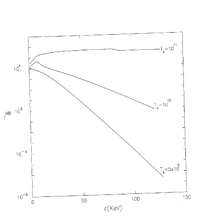
Figure 1: $I^{MB}(in\ \ ergs\ cm^{-2}S^{-1}HZ^{-1}Str^{-1})$ versus photon energy $\epsilon$ in KeV, for temperatures $T_{e}$= 5 $\times$ 10⁹K, 10¹⁰ K, 10¹¹K

Figure 2: (a) $I^{-}$ the emergent intensity (in the direction of $\tau\rightarrow 0$) at different layers at $N$=50 ($\tau=\tau_{max}$), $N$=25($\tau=0.5$) and $N$=1 ($\tau=0$) for angle $\mu_{1}$ for temperature $5\times 10^{9}$ K. (b) $I^{+}$ the reflected intensities at N=50, 25, and 1. The initial incident intensity is $I^{-}(N=50)=1$. (c) and (d): shows the photon phase densities $n^{-}$ and $n^{+}$ corresponding to $I^{-}$ and $I^{+}$ given in figures (a) and (b) respectively

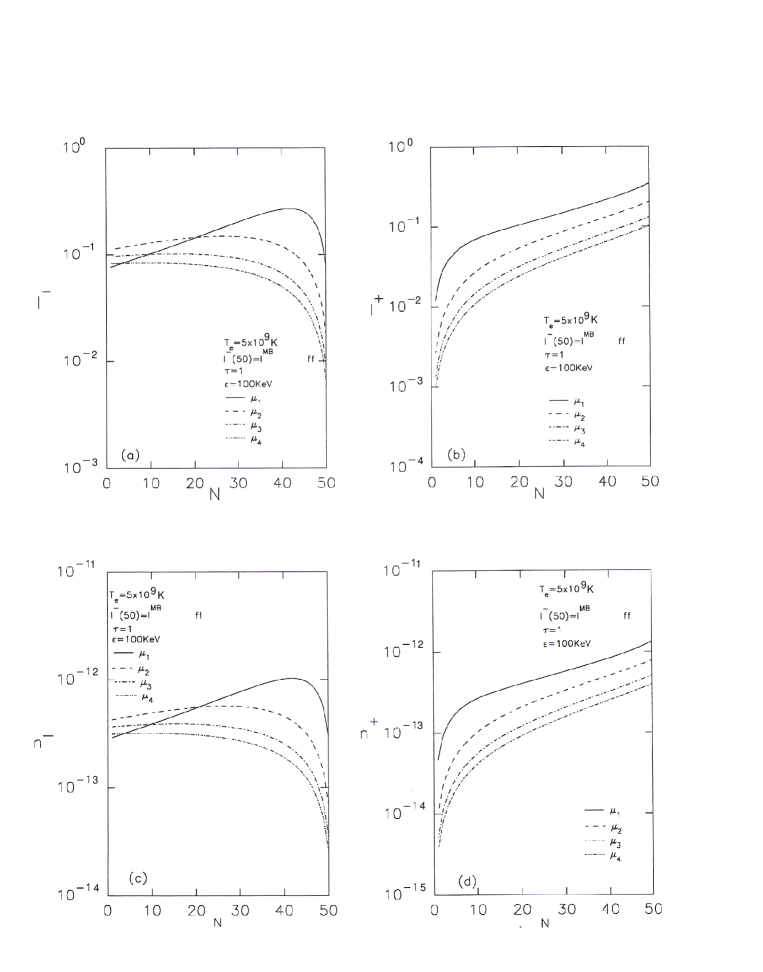
Figure 3: The transfer of photon with $\epsilon$=100 KeV energy across the medium from $N=50$ to $N=1$, in a medium with free-free emission and $I^{-}(N=50)=I^{MB}$ as the initial intensity.

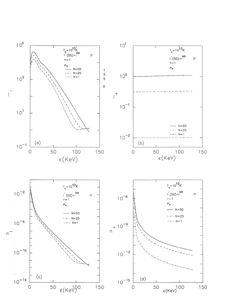
Figure 4: Same as those given in figure 3, but with $T_{e}$=10${}^{10}K$

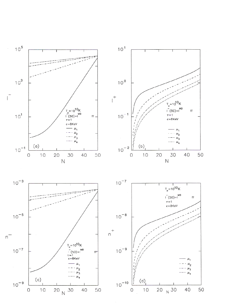
Figure 5: The transfer of photon with $\epsilon$=8 KeV energy across the medium from $N=50$ to $N=1$, in a medium with free-free emission and $I^{-}(N=50)=I^{MB}$ as the initial intensity for $T_{e}$=10${}^{10}K$

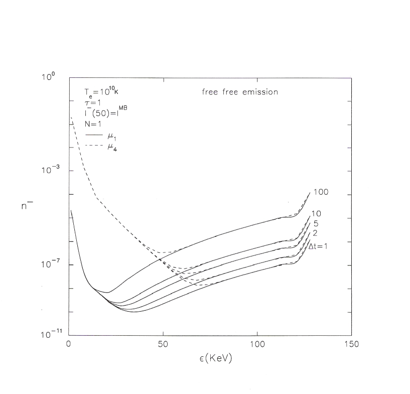
Figure 6: The photon phase density $n^{-}$ corresponding to $I^{-}$ is given versus $\epsilon$. The enhancement of $n^{-}$ for $\delta t$=1, 2, 5, 10, 100 is shown. The incident radiation is $I^{-}(N=50)=I^{MB}$ in a medium with free-free emission

Figure 7: The emergent and reflected intensities $I^{-}$ and $I^{+}$ with initial condition $I^{-}(N=50)=I^{MB}\times C_{\mu}$where $C_{\mu}=\displaystyle{\frac{6}{3+2b}}\bigg{(}\mu+b\mu^{2}\bigg{)}$

Figure 8: Same as those given in figure 7 with $I^{-}(N=50)=I^{MB}\times D_{\mu}$ where $D_{\mu}=2\mu\ ln\ \bigg{(}\frac{1+\mu}{\mu}\bigg{)}$

4 Conclusions

Using discrete space theory of radiative transfer comptonization spectra is calculated in a plane parallel atmosphere with isotropic and anisotropic as a incident radiation. The accuracy of the solution is assumed by observing 1)strict radiant flux conservation 2) non-negativety and continuity of the solution across $(-1\leq\mu\leq 1)$ by taking the step size for the democratization. We estimated the photon phase densities from the specific intensities which is calculated from radiative transfer equation and the time evolution of photon phase density by employing Kompaneets equation. There is substantial differences are noticed in the nature of emergent intensity variations with free-free emissions and absorption cases. We also studied when a photon of given energy would get transformed through the medium and noticed that when transfer takes place radiation field becomes angle dependent. We noticed that the initial spectrum is angle dependent and the Kompaneets equation gives a angle independent spectrum after many Compton scatterings. We are plan to extend the above method for spherically symmetric approximation to study the stellar atmospheres in X-ray binaries and accretion discs atmospheres in active galatic nuclei(AGN) etc.

5 Acknowledgements

Authors would like to thank Prof M. Pinar Menguc for his remarks made on the manuscript which improved the clarity of the paper. We also would like to thank the anonymous referee for his strong comments, suggestions and for his patience which improved the quality of the paper.

Appendix A

Equation (29) can be solved numerically by using discrete space theory of radiative transfer [60], [61], and [62]. We discritise the equation (29) on the $[x_{(}i)-z(n)-\mu(m)]$ discrete mesh and this becomes

$${\bf M}_{m}\bigg{[}{\bf I}^{+}_{i,n+1}-{\bf I}^{+}_{i,n}\bigg{]}+\tau_{n+\frac{1}{2}}\sigma_{i}^{+}{\bf I}^{+}_{i,n+\frac{1}{2}}$$ (42)

$$= \tau_{n+\frac{1}{2}}\bigg{[}\sigma_{a}{{\bf B}^{\prime}_{\epsilon,i,{n+\frac{1}{2}}}}+\sigma_{a}^{ff}{{\bf B}^{ff}_{em,i,{n+\frac{1}{2}}}}\bigg{]}{\bf h}$$

$$+ \frac{3}{64\pi}\tau_{n+\frac{1}{2}}\bigg{[}{\bf R}^{++}_{i,i^{\prime},{n+\frac{1}{2}}}\ {\bf a}^{++}_{i^{\prime},{n+\frac{1}{2}}}{\bf CI}^{+}_{i^{\prime},{n+\frac{1}{2}}}$$

$$+ {\bf R}^{+-}_{i,i^{\prime},{n+\frac{1}{2}}}\ {\bf a}^{+-}_{i^{\prime},{n+\frac{1}{2}}}{\bf CI}^{-}_{i^{\prime},{n+\frac{1}{2}}}\bigg{]}$$

$${\bf M}_{m}\bigg{[}{\bf I}^{-}_{i,n}-{\bf I}^{-}_{i,n+1}\bigg{]}+\tau_{n+\frac{1}{2}}\sigma_{i}^{-}{\bf I}^{-}_{i,n+\frac{1}{2}}$$ (43)

$$= \tau_{n+\frac{1}{2}}\bigg{[}\sigma_{a,i}{{\bf B}^{\prime}_{\epsilon,i,{n+\frac{1}{2}}}}+\sigma_{a,i}^{ff}{{\bf B}^{ff}_{em,i,{n+\frac{1}{2}}}}\bigg{]}{\bf h}$$

$$+ \frac{3}{64\pi}\tau_{n+\frac{1}{2}}\bigg{[}{\bf R}^{-+}_{i,i^{\prime},{n+\frac{1}{2}}}\ {\bf a}^{-+}_{i^{\prime},{n+\frac{1}{2}}}{\bf CI}^{+}_{i^{\prime},{n+\frac{1}{2}}}$$

$$+ {\bf R}^{--}_{i,i^{\prime},{n+\frac{1}{2}}}\ {\bf a}^{--}_{i^{\prime},{n+\frac{1}{2}}}{\bf CI}^{-}_{i^{\prime},{n+\frac{1}{2}}}\bigg{]}$$

where

$${\bf B}^{\prime}_{em,i,{n+\frac{1}{2}}}=\frac{{\bf B}_{e}(x_{i},\beta)}{n_{e},{n+\frac{1}{2}}\sigma_{T}}$$

$${\bf M}_{m}=\bigg{[}\mu_{m}\delta_{mk}\bigg{]}$$ (44)

$${\bf C}=\bigg{[}c_{m}\delta_{mk}\bigg{]}$$ (45)

$${\bf h}=\bigg{[}1,1,1,\ldots\bigg{]}^{T}_{m}$$ (46)

T represents the transpose and $\mu$’s and C’s are the roots and weights of angle quadrature and

$$\tau_{n+\frac{1}{2}}=n_{\epsilon}\sigma_{T}\Delta Z$$ (47)

$${\bf I}^{\pm}_{i,n}={\bf I}(x_{i},\pm\mu_{m},Z_{n})$$ (48)

$$\sigma^{\pm}_{i} = \sigma(\pm x_{i})$$ (49)

$$= \sigma(x\pm\mu\beta)$$

$${\bf R}^{++}_{i,i^{\prime},{n+\frac{1}{2}}}=$$

$$\frac{1}{x_{i^{2}}}\bigg{[}\frac{x_{i}}{x_{i^{\prime}}}+\frac{x_{i^{\prime}}}{x}-2\bigg{(}\frac{1}{x_{i^{\prime}}}-\frac{1}{x_{i}}\bigg{)}+\bigg{(}\frac{1}{x_{i^{\prime}}}-\frac{1}{x_{i}}\bigg{)}^{2}\bigg{]}_{n+\frac{1}{2}}$$ (50)

Similarly ${\bf R}^{+-},{\bf R}^{-+}$ and ${\bf R}^{--}$. In case of static medium,

$${\bf R}^{++}={\bf R}^{+-}={\bf R}^{-+}={\bf R}^{--}$$ (51)

The subscript ${n+\frac{1}{2}}$ refers to the average of the layer with boundaries $Z_{n}$ and $Z_{n+1}$. If we write

$${\bf M} = \left(\begin{array}[]{cccc}{\bf M}_{m}&&&\\ &{\bf M}_{m}&&\\ &&\ddots&\\ &&&\quad{\bf M}_{m}\end{array}\right),$$ (56)

$${\bf C} = \left(\begin{array}[]{cccc}{\bf C}^{+}_{m}&&&\\ &{\bf C}^{+}_{m}&&\\ &&\ddots&\\ &&&\quad{\bf C}^{+}_{m}\end{array}\right),$$ (61)

$${\bf W}_{kk^{\prime}}=a_{i}c_{j}=\frac{A_{i}R_{kk^{\prime}}c_{j}}{\sum R_{kk\prime}A_{i}c_{j}}\quad\quad\quad\quad a_{i}=\frac{A_{i}R_{kk^{\prime}}}{\sum R_{kk^{\prime}}A_{i}c_{j}}$$ (62)

then equations (A.1) and (A.2) would become for ${\bf I}^{\prime}$ energy points.

$${\bf M}\bigg{[}{\bf I}^{+}_{n+1}-{\bf I}^{+}_{n}\bigg{]}+\tau_{n+\frac{1}{2}}\sigma^{+}_{n+\frac{1}{2}}{\bf I}^{+}_{n+\frac{1}{2}}$$ (63)

$$= \tau_{n+\frac{1}{2}}{\bf S}^{+}_{n+\frac{1}{2}}+\tau_{n+\frac{1}{2}}\eta\bigg{[}{\bf R}^{++}{\bf W}^{++}{\bf I}^{+}+{\bf R}^{+-}{\bf W}^{+-}{\bf I}^{-}\bigg{]}_{n+\frac{1}{2}}$$

$${\bf M}\bigg{[}{\bf I}^{-}_{n}-{\bf I}^{-}_{n+1}\bigg{]}+\tau_{n+\frac{1}{2}}{\bf I}^{-}_{n+\frac{1}{2}}$$ (64)

$$= \tau_{n+\frac{1}{2}}{\bf S}^{-}_{n+\frac{1}{2}}+\tau_{n+\frac{1}{2}}\eta\bigg{[}{\bf R}^{-+}{\bf W}^{-+}{\bf I}^{+}+{\bf R}^{--}{\bf W}^{--}{\bf I}^{-}\bigg{]}_{n+\frac{1}{2}}$$

where

$$\eta=\frac{3}{64\pi}$$ (65)

$$\bf I^{\pm}_{n}=\left(\begin{array}[]{c}I^{\pm}_{1,n}\\ I^{\pm}_{2,n}\\ I^{\pm}_{3,n}\\ \ldots\\ I^{\pm}_{I^{\prime},n}\end{array}\right)$$ (66)

$${\bf S}_{n+\frac{1}{2}}=\bigg{[}\sigma_{a}{\bf B}^{\prime}_{em,i,{n+\frac{1}{2}}}+\sigma^{ff}_{a}{\bf B}^{ff}_{emi,{n+\frac{1}{2}}}\bigg{]}\left(\begin{array}[]{c}1\\ 1\\ 1\\ \ldots\\ 1\end{array}\right)_{I^{\prime}}$$ (72)

If we use ”diamond scheme” [62]

$${\bf I}^{\pm}_{n+\frac{1}{2}}=\frac{1}{2}\bigg{(}{\bf I}^{\pm}_{n}+{\bf I}^{\pm}_{n+1}\bigg{)}$$ (73)

and we write the equation (A.13) and (A.14) in the form of interaction principle. We obtain

$$\left(\begin{array}[]{cc}X11&X12\\ X21&X22\\ \end{array}\right)\left(\begin{array}[]{c}I^{+}_{n+1}\\ \\ I^{-}_{n\ \ }\end{array}\right)$$ (79)

$$=\left(\begin{array}[]{cc}Y11&Y12\\ Y21&Y22\\ \end{array}\right)\left(\begin{array}[]{c}I^{+}_{n}\\ \\ I^{+}_{n+1\ \ }\end{array}\right)$$ (85)

$$+\tau\left(\begin{array}[]{c}S^{+}\\ S^{-}\\ \end{array}\right)$$ (88)

where

$$X11={\bf M}+\displaystyle\frac{1}{2}\tau\bigg{(}\sigma^{+}-\eta R^{++}W^{++}\bigg{)}$$

$$X12=-\displaystyle\frac{1}{2}R^{+-}W^{+-}$$

$$X21=-\displaystyle\frac{1}{2}\tau R^{-+}W^{-+}$$

$$X22={\bf M}+\displaystyle\frac{1}{2}\tau\bigg{(}\sigma^{-}-R^{--}W^{--}\bigg{)}$$

$$Y11={\bf M}-\displaystyle\frac{1}{2}\tau\bigg{(}\sigma^{+}-{\frac{-1}{2}}R^{++}W^{++}\bigg{)}$$

$$Y12=+\displaystyle\frac{1}{2}\tau R^{+-}W^{+-}$$

$$Y21=+\displaystyle\frac{1}{2}\tau R^{-+}W^{-+}$$

$$Y22={\bf M}-\displaystyle\frac{1}{2}\tau\bigg{(}\sigma^{-}-R^{--}W^{--}\bigg{)}$$

We can derive the transmission and reflection matrices and the source vectors, from the equation (A.19) by the comparison with the interaction principle [62] and are given in the Appendix.

To calculate the diffuse radiation ie., the specific intensities at each spacial point in the medium, ${\bf I}^{\pm}_{n}$, we use the scheme described in [63]and [62]. We estimate ${\bf I}^{+}_{n+1},{\bf I}^{-}_{n}$ at each point which are given by,

$${\bf I}_{n+1}^{+}=r(1,n+1){\bf I}^{-}_{n+1}+{\bf V}^{+}_{n+\frac{1}{2}}$$ (89)

$${\bf I}_{n}^{-}=t(n,n+1){\bf I}^{-}_{n+1}+{\bf V}^{-}_{n+\frac{1}{2}}$$ (90)

where $r(1,n+1),t(n,n+1)$ are the diffuse reflection and transmission matrices at the internal points. ${\bf V}^{+}_{n+\frac{1}{2}},{\bf V}^{-}_{n+\frac{1}{2}}$ are the source vectors which represent the emission from the layer whose boundaries are $Z_{n}$ and $Z_{n+1}$ together with the diffuse radiation from the rest of the medium.

The quantity ${\bf I}^{+}_{n+1}$ represents the reflected intensity in the direction of increasing $\tau(\tau\rightarrow{\bf T}$, the total optical depth) while ${\bf I}^{-}_{n}$ represents the emergent intensity toward decreasing $\tau\rightarrow 0$. We can estimate these two quantities through the equations (A.20) and (A.21) at any spacial point in the medium in the form of angular distribution.

The transmission and reflection operators as are given by,

$${\mbox{\boldmath$t$}}(n+1,n)={\bf G}^{+-}\bigl{[}\Delta^{+}\bf A^{+}+g^{+-}+\bf g^{-+}\bigr{]}$$

$${\mbox{\boldmath$r$}}(n+1,n)={\bf G}^{-+}\bf g^{-+}\bigl{[}{\bf E}+\Delta^{+}{\bf A}^{+}\bigr{]}$$

$${\mbox{\boldmath$t$}}(n,n+1)={\bf G}^{-+}\bigl{[}\Delta^{-}\bf A^{-}+\bf g^{-+}g^{+-}\bigr{]}$$

$${\mbox{\boldmath$r$}}(n,n+1)={\bf G}^{+-}\bf g^{+-}\bigl{[}{\bf E}+\Delta^{-}{\bf A}^{-}\bigr{]}$$

Where ${\bf E}$ is identity matrix and

$${\bf G}^{+-}=\bigl{[}{\bf E}-\bf g^{+-}\bf g^{-+}\bigr{]}^{-1}$$

$${\bf G}^{-+}=\bigl{[}{\bf E}-\bf g^{-+}\bf g^{+-}\bigr{]}^{-1}$$

$$\bf{g}^{+-}=\frac{1}{2}\tau\Delta^{+}$$

$$\bf{g}^{-+}=\frac{1}{2}\tau\Delta^{-}{\bf Y}$$

$${\Delta}^{+}=\bigl{[}{\bf M}+\frac{1}{2}\tau{\bf Z}\bigr{]}^{-1};\quad{\bf Z}=\sigma-\eta{\bf R}{\bf W};\quad{\bf Y}=\eta{\bf R}{\bf W}$$

and the source vectros are,

$$\Sigma^{+}=\tau{\bf G}^{+-}\bigl{[}\Delta^{+}+\bf g^{+-}\bf\Delta^{-}\bigr{]}{\bf S}$$

and

$$\Sigma^{-}=\tau{\bf G}^{-+}\bigl{[}\Delta^{-}+\bf g^{-+}\bf\Delta^{+}\bigr{]}{\bf S}$$

${\bf S}$ being the source function.

References

• [1] Rybieki, G. B., Lightman, A. P., 1979, Radiative Prcesses in Astrophysics, John Wiley & Sons, Newyork
• [2] Lightman, A. P., Rybicki, G. B., Inverse Compton reflection - The steady-state theory, 1980, ApJ, 236, 928
• [3] Kershaw, Davia. S., Prasad, J., Manoj, K., A simple and fast method for computing the relativistic Compton Scattering Kernel for Radiative transfer, 1986, JQSRT, Vol 36, No 4, 273-282
• [4] Prasad, M. K., Shestakov, A. I., Kershaw, D. S., and Zimmerman, G. B, Diffusion coefficient for the Compton Fokker-Planck Equation, 1988, JQSRT, Vol 40, No 1, 29-38
• [5] Larsen, E. W., Levermore, C. D., Pomraning., Discretization Methods for One-Dimensional Fokker-Planck Operators, 1985, J. Comp. Phys., 61, 359-390,
• [6] Ghisellini, G., George, I. M., Fabian., A. C., Done, C., Anisotropic inverse Compton emission, 1991, MNRAS, 248,14
• [7] Piro, L., Matsuoka, M., Yamauchi, M., 1989, in Hunt, J., Battrick, B., Eds. Proc. 23rd ESLAB Symp. on Two-Topics in X-ray Astronomy, ESA SP-296, ESTEC, Noordwijk, The Netherlands, P819
• [8] Pounds, K. A., Nandra, K., Steward, G. C., George., I. M., fabian, A. C., X-ray reflection from cold matter in the nuclei of active galaxies, 1990, Nat, 344, 132
• [9] Nandra, K., Pounds, K., GINGA Observations of the X-Ray Spectra of Seyfert Galaxies, 1994, MNRAS, 268, 405
• [10] Done, C., Mulchaey, J. S., Mushotzky, R. F., & Arnaud, K. A., An ionized accretion disk in Cygnus X-1, 1992, ApJ, 395,275
• [11] Haardt, F.; Done, C.; Matt, G.; Fabian, A. C.,The high-energy spectrum of Cygnus X-1 revisited, 1993ApJ…411L..95H
• [12] Illarionov, A. F., Kallman, T., McCray, R., Ross,R., Comptonization of X-rays by low-temperature electrons, 1979, ApJ, 228, 279
• [13] Canfield, E., Howard, W. M., Liang, E. P., Inverse Compton by one-dimensional relativistic electrons, 1987, December 15., ApJ, 323, 565-574
• [14] George, I. M., Fabian, A. C., X-ray reflection from cold matter in active galactic nuclei and X-ray binaries, 1991, MNRAS, 249, 352
• [15] Matt, G., Perola, G. C., Piro, L, The iron line and high energy bump as X-ray signatures of cold matter in Seyfert 1 galaxies, 1991, A & A, 247, 25
• [16] Hua, X.-M., Lingenfelter, R. E., Angle-dependent Green’s functions for relativistic Compton reflection, 1992, ApJ, 397,591
• [17] Ghisellini, G., Haardt, F., Matt, G., The Contribution of the Obscuring Torus to the X-Ray Spectrum of Seyfert Galaxies - a Test for the Unification Model, 1994, MNRAS, 267, 743
• [18] Burigana, C., Ai semi-analytical solution of the transfer equation for Compton reflection models, 1995, MNRAS, 272, 481
• [19] Magadziarz, P., Zdziarski, A. A., Angle-dependent Compton reflection of X-rays and gamma-rays, 1995, MNRAS, 273,837
• [20] Lightman, A. P.; Lamb, D. Q.; Rybicki, G. B., Comptonization by cold electrons, 1981ApJ…248..738
• [21] White, T. R., Lightman, A. P., Zdziarski, A, A., Compton reflection of gamma rays by cold electrons, 1988, ApJ, 331, 939
• [22] Czerny, B., Elvis, M., Constraints on quasar accretion disks from the optical/ultraviolet/soft X-ray bi bump, 1987, ApJ, 321, 305
• [23] Zdziarski, Andrzej A.; Ghisellini, Gabriele; George, Ian M.; Fabian, A. C.; Svensson, Roland; Done, Chris Electron-positron pairs, Compton reflection, and the X-ray spectra of active galactic nuclei, 1990ApJ…363L…1Z
• [24] Haardt, F., Marasachi, L., A two-phase model for the X-ray emission from Seyfert galaxies, 1991, ApJ, 380, L51
• [25] Sunyaev, R. A., Titarchuk, L. G., Comptonization of X-rays in plasma clouds - Typical radiation spectra, 1980, A & A, 86, 121
• [26] Rogers, R. D., Field, G. B., Compton reflection in active galactic nuclei and the cosmic X-ray background, 1991, ApJ, 370, L57
• [27] Haardt, F., Anisotropic Comptonization in thermal plasmas - Spectral distribution in plane-parallel geometry, 1993ApJ…413..680H
• [28] Nishimura, J., Mitsuda, K., Itoh, M., Comptonization of soft X-ray photons in an optically thin hot plasma, 1986, PASJ, 38, 819
• [29] Miyamoto, S., Radiative transfer effect in an ionized medium at high temperature, 1978, A & A, 63, 69
• [30] Katz, J., Nonrelativistic Compton scattering and models of quasars, 1976, ApJ, 206, 910
• [31] Shapiro, S., Lightman, A., Eardley, D., A two-temperature accretion disk model for Cygnus X-1 - Structure and spectrum, 1976, ApJ, 204, 187
• [32] Pozdniakov, L. A., Sobol, I. M., Syunyaev, R. A., Comptonization and the shaping of X-ray source spectra - Monte Carlo calculations, 1983ASPRv…2..189P,
• [33] Kompaneets, A. S., 1956. Zh.E.F.T., 31, 876. Translation Establishment of thermal equilibrium between quanta and electrons, Soviet Physics JETP, 4, (1957), pp. 730-737.
• [34] Illarionov, A. F., Syunyaev, R. A., Compton Scattering by Thermal Electrons in X-Ray Sources, 1972, Soviet Astronomy, 16, 45
• [35] Sunyaev, R. A., Titarchuk, L. G., Comptonization of low-frequency radiation in accretion disks Angular distribution and polarization of hard radiation, 1985, A & A, 143, 374
• [36] Wehrse, R., Hof, M., 1990, Conference Proceedings 232 on Gamma-Ray line Astrophysics, Ed. P. Durouchoux and Prantzos, Page 477
• [37] Madej, J, Tables of Model Atmospheres of Bursting Neutron Stars, Vol, 41, No. 2., 1991, Acta Astronomica, P. 73
• [38] Madej, J, Model Atmospheres and X-ray Spectra of Bursting Neutron Stars, ApJ, 1991, 376, P.161
• [39] Madej, J.; RΓ³ΕΌaΕ„ska, A., X-ray irradiated model stellar atmospheres, A&A, 2000, 356, 654M
• [40] Madej, J.; RΓ³zaΕ„ska, A, X-ray irradiated model stellar atmospheres. II. Comprehensive treatment of Compton scattering, A & A, 2000, 363, 1055M
• [41] Joss, Paul C., Madej, Jerzy., Theoretical Spectra of Unmagnetized Neutron Stars, tysc.confE, 2001, 214J
• [42] Deufel, B., Dullemond, C. P., & Spruit, H. C., X-ray spectra from accretion disks illuminated by protons, 2002, A&A, 387, 907
• [43] Madej, J.; Joss, P. C.; RΓ³ΕΌaΕ„ska, A., Model Atmospheres and X-Ray Spectra of Bursting Neutron Stars: Hydrogen-Helium Comptonized Spectra, 2004, ApJ…602..904M
• [44] Madej, J.; RΓ³ΕΌaΕ„ska, A, X-ray irradiated model stellar atmospheres - III. Compton redistribution of thermal external irradiation, 2004,MNRAS.347.1266M
• [45] Majczyna, A., Madej, J., Joss,, P. C., and Rozanska, A., Model atmospheres and Xray Spectra of Bursting neutron stars II . Iron rich comptonized spectra, A&A, 2005, 643
• [46] Suleimanov, V.; Madej, J.; Drake, J. J.; Rauch, T.; Werner, K. On the relevance of Compton scattering for the soft X-ray spectra of hot DA white dwarfs, 2006A&A…455..679S
• [47] Suleimanov, V.; Madej, J.; Drake, J. J.; Rauch, T.; Werner, K. Soft X-ray spectra of hot DA white dwarfs with Compton Scattering, 2007, ASPC..372..217S
• [48] Guilbert, P. W., Numerical solution of time dependent Compton scattering problems by means of an integral equation, 1981MNRAS.197..451G
• [49] Chluba, J.; Sunyaev, R. A.,Evolution of low-frequency features in the CMB spectrum due to stimulated Compton scattering and Doppler broadening, 2008, A&A…488..861C
• [50] Dubinov, A. E, Exact Satationary Solution of the Kompaneets Kinatic Equation, Technical Physical Letters, 2009, Vol. 35, No. 3, P260
• [51] Procopio, P.; Burigana, C., A numerical code for the solution of the Kompaneets equation in cosmological, 2009, A&A…507.1243P
• [52] Zeldovich, Ya. B., Levich, E. V., Stationary state of electrons in a non-equilibrium radiation field, 1970, JETP, LEtt., 11, 35
• [53] Levich, E. V., Syunaev, R. A., Heating of Gas near Quasars, Seyfert-Galaxy Nuclei, and Pulsars by Low-Frequency Radiation. 1971, SoV. Astron-Aj, 15, 363
• [54] Dreicer, H.,netic Theory of an Electron-Photon Gas, 1964, Phys. Fluids, 7, 735
• [55] Arons, J., Radiative Transfer of Isotropic X-Rays and Gamma Rays. I. General Theory and Solutions for a Uniform Medium,1971, ApJ, 164,437
• [56] Evans, R. D., 1958, Handbuch der Physik, 218, ed S. Flugge, Springer Verlag
• [57] Jauch, J. M., Rohrlich, F., Theory of photons and Electrons,(reading, Mass: Addison-Wesley)
• [58] Chandrasekhar, S., Stochastic Problems in Physics and Astronomy, 1943, Rev. Mod. Phys, 15, 1
• [59] Pomraning, G. C., Freeman, B. E., The equation of radiative transfer with scattering, 1968, JQSRT, 8, issue 3, 909
• [60] Grant, I. P., Peraiah, A., Spectral line formation in extended stellar atmo-spheres, 1972, MNRAS, 160,239
• [61] Peraiah, A., Wehrse, R., Formation of the Hydrogen Lyman Β  Line in Expanding Spherical Nebulaei, 1978, A & A., 70, 213
• [62] Peraiah, A., 2002, ”An introduction to radiative transfer: Methods and applications in astrophysics” Cambridge University press
• [63] Grant, I. P., Hunt, G. E., Solution of radiative transfer problems using the invariant Sn method, 1968, MNRAS, 141, 27