LIGHT CURVE SOLUTIONS OF ECLIPSING BINARIES IN SMC

Abstract

We propose a procedure for light-curve solution of eclipsing binary stars in the Small Magellanic Cloud for which photometric data have been obtained in the framework of the OGLE project as well as way of determination of the global stellar parameters on the basis of the obtained solutions, some empirical relations as well as the distance to the SMC. Several examples illustrate this procedure.

1 Introduction

The microlensing experiments monitor very crowded fields and after several years they lead to recording of variability of a huge number of objects and epochs. As a result, the ability to generate data far exceeds the ability to process it. The microlensing project OGLE (Optical Gravitational Lensing Experiment) as well as the projects EROS (Grison et al. 1995) and MACHO (Alcock et al. 1997) monitored millions of stars in the Magellanic Clouds during the last two decades. This large photometric database is available not only for microlensing studies but also for individual and statistical investigations of variable stars.

The OGLE data have been obtained by 1.3-m Warsaw telescope at Las Campanas Observatory (Chile) equipped with CCD mosaic camera 8kMOSAIC consisting of eight thin SITe 2048 x 4096 CCD chips. The majority of observations are made in $I$ color. The main results from the analysis of the OGLE observations are detections of: gravitational lensing events; planetary and low luminosity object transits; small amplitude variable red giants in the Magellanic Clouds; eclipsing stars in the SMC; RR Lyr stars in the LMC; population II Cepheids in the Galactic Bulge (Paczynski et al. 1999); stellar proper motion; star clusters, etc. In particular, the OGLE II project (Udalski et al. 1997) provided $BVI$ light curves for about several millions of stars from the central parts of the Magellanic Clouds (Udalski et al. 1998, 2000).

The sample of 68000 variable stars detected in LMC and SMC (Graczyk 2003) is reasonably complete allowing statistical analysis and provides a good material for testing the evolutionary theory of the binary systems, studying the evolution of the Magellanic Clouds, star formation, etc. The future spectral observations of the eclipsing binaries with 8-m European Southern telescopes in Chile will allow to study the geometrical and spatial distribution of the stars in these galaxies.

2 OGLE catalogue of eclipsing binary stars in the SMC

The search for variable stars in the Magellanic Clouds in the framework of the OGLE project has been performed automatically using $I$-band data from 140-180 epochs (with lower limit set of 50) with the software DIA (Difference Image Analysis). The light curves of the selected candidates are searched for periodicity using the AoV algorithm (Zebrun et al. 2001).

Udalski et al. (1998) presented the first catalogue of about 1500 eclipsing stars found in the central 2.4 square degree area of the SMC brighter than $I=20^{m}$ with periods from 0.3 days to 250 days. The next catalogue of variable stars in the Magellanic Clouds found on OGLE-II data in 1997-2000 (Zebrun et al. 2001) covers about 7 square degrees of the sky (21 fields in the LMC and 11 fields in the SMC). This catalogue is available in electronic form: http://www.astrouw.edu.pl/ ftp/ogle or http://www.astro.princeton.edu/ ogle.

The OGLE catalogue of the eclipsing binary stars in the SMC contains 1350 objects of different types. Some of them reveal eccentric orbits with possible apsidal motion. The binaries are sorted by type (EA, EB, EW, approximately corresponding to detached, semi-detached and contact binaries) as well as by the field they are located in. The catalogue contains the following information: number of the star; OGLE-II field; name of the star; RA; DEC; x and y coordinates in the reference image; orbital period; HJD for the primary maximum (T - 2450000); zero epoch (phase 0) corresponding to the deeper eclipse; $I$-band brightness at maximum; $I$-band amplitude (depth of the primary minimum); phase of the secondary eclipse; depth of the secondary eclipse in $I$ band; $I$, $B$ and $V$ brightness at maximum; $(B-V)$ and $(V-I)$ color indices; type of the eclipsing star. Clicking the star name provides its photometry in the following format: HJD, magnitude and magnitude error. The errors of magnitude measurements are: 0.005^m for the brightest stars $(I<$15${}^{m})$; 0.08^m for stars with 15${}^{m}<I<$19^m; 0.3^m for stars with 20.5${}^{m}<I$. Typically, there are about 400 data points in $I$ band and about 30-40 points in $V$ and $B$ band for each variable in the catalogue.

3 Procedure of light curve solution

The light curve solution presents searching for the best coincidence between a family of theoretical light curves corresponding to different values of the star parameters with observed photometric data. It is based on the least squares method and the searched solution is that for which the sum of the residuals is minimum.

Taking into account the quality of the OGLE data we propose a procedure of light curve solution for the eclipsing binaries in SMC containing four stages:

(a) preliminary light curve solution on the basis of known statistical relations between the global stellar parameters (Kjurkchieva et al. 2006, 2007, 2008);

(b) initial light curve solution by the code Binary Maker 3 (Bradstreet $\&$ Steelman 2004) for determination of relative stellar radii $r_{1}$ and $r_{2}$, temperatures $T_{1}$ and $T_{2}$, mass ratio $q$, orbital inclination $i$, eccentricity $e$ and (eventually) spot parameters;

(c) final multicolor solution using the code DC (Wilson $\&$ Van Hamme 2003) or PHOEBE (Prsa $\&$ Zwitter 2005) to determine the varied parameters and their errors;

(d) calculation of the global stellar parameters on the basis of some empirical relations as well as the distance to the binary, i.e. to the SMC (Graczyk 2003).

3.1 Preliminary solution

The goal of this stage is to get some preliminary values of the stellar parameters.

The reducing of the catalogue data includes the following steps:

(a) creating the .dat file (phase/flux) from the observed data in the form JD/magnitude (the value 1 of the flux should correspond to the middle level at the phase of maximum brightness in $I$ color);

(b) visualization of the .dat file and removing the points that are far outside the common course of light variability;

(c) measurement of the fluxes $l_{1}$ and $l_{2}$ at the bottoms of the two $I$ minima;

(d) visual estimation of the maximum observed out-of-eclipse flux in $I$, $B$ and $V$ colors;

(e) determination of the $(B-V)_{0}$ index by the formula (Harries et al. 2003)

$$(B-V)_{0}=(B-V)-E_{B-V}=(B-V)-A_{V}/R$$ (1)

where $R$=3.1 is the mean total extinction to SMC (Bouchet et al. 1985) and $A_{V}$ is the local extinction to the region surrounding the target binary determined by 30 stars (Zaritsky et.al 2002). The values of $A_{V}$ could be taken from SMC Extinction Retrieval Service: http://ngala.as.arizona.edu/dennis/smcext.html.

Then the determination of the preliminary stellar parameters goes in the following order:

(a) determination of the mean temperature of the binary $T_{0}$ by the empirical relation ${T_{0}}/{(B-V)_{0}}$ built on the calibration of Flower (1996) for the Galactic stars;

(b) calculation of the initial temperature of the secondary star $T_{02}$ by the formula (Bronstein 1972):

$$T_{02}\approx T_{01}\bigg{(}{\frac{1-l_{2}}{1-l_{1}}}\bigg{)}^{1/4}$$ (2)

adopting that the initial primary-star’s temperature $T_{01}$ is equal to the mean temperature of the binary $T_{0}$, i.e. $T_{01}$=$T_{0}$;

(c) calculation of the initial mass ratio $q_{0}$ by the empirical relation (Kjurkchieva $\&$ Ivanov 2006):

$$q_{0}=M_{2}/M_{1}\approx(T_{02}/T_{01})^{1.7};$$ (3)

(d) calculation of the ratio of relative radii by the empirical relation (Kjurkchieva $\&$ Ivanov 2006):

$$r_{2}/r_{1}=R_{2}/R_{1}\approx q_{0}^{0.75}.$$ (4)

3.2 Initial light curve solution

In order to get fast, initial, light-curve solution we propose to use the code Binary Maker 3 (BM3) because it allows to see immediately the effect of changing of each parameter on the synthetic light curve (Bradstreet & Steelman 2004). The visualization is very useful tool at this stage of trials and errors.

To obtain synthetic light curve by BM3 one should insert: (a) the preliminary values of the star parameters obtained by the empirical relations (stage 1); (b) tabular values of the limb darkening, gravitation darkening and reflection coefficients appropriate to the initial temperatures of the stellar components; (c) some suspected value of the orbital inclination.

To get better coincidence of the theoretical light curve with the photometric points one should begin to vary the configuration parameters by trials and errors. Besides the visual estimation of the fit quality the code BM3 provides the sum of the O-C residuals as an objective criterion.

We note that: (a) at this stage good fit is searched only in $I$ color because there are a few $B$ and $V$ data of the OGLE catalogue; (b) the primary’s temperature remains fixed at this stage of procedure; (c) if the observed light curve is asymmetric and/or distorted one should try solution with surface spots varying their parameters.

Our experience in the light curve analysis leads to the following recommendations: (a) The wanted widths of the eclipses may be reached varying the relative radii; (b) Simultaneous increase/decrease of the depths of the two minima may be provided by increase/decrease of the orbital inclination; (c) The increase/decrease of the relative depth of the secondary minimum can be provided by increase/decrease of the temperature of the secondary star; (d) Spots with longitudes around $90^{\circ}$ and $270^{\circ}$ change the out-of-eclipse light levels while spots with longitudes around $0^{\circ}$ and $180^{\circ}$ change the shape and depth of the corresponding eclipse. As a rule, the longitude of the spot center corresponds to the maximum of the light curve distortion.

If the foregoing procedure leads to solution with $q>1$ then the parameters of the two stars (temperatures, darkening coefficients, albedoes and relative radii) should be exchanged $by$ $hand$. This is necessary because we assume that the primary star is eclipsed during the deeper minimum while BM3 assumes as a primary star that with bigger mass.

After reaching a good $I$-band solution one should obtain (by BM3) the corresponding $V$ and $B$ synthetic curves. Usually they reproduce well the observational points (when the corresponding stars emit as black body). Moreover, the good coincidence in $V$ and $B$ bands means that we have determined well the maximum light in $B$ and $V$ colors. If this is not the case, we should search for a better coincidence of the light curves in all three colors simultaneously varying the normalization level of the respective curve ($B$ or/and $V$) on the basis of visual estimation. This leads to some correction of the color index as well as the primary temperature and consequently to repeating of the whole procedure but varying the parameters in quite narrow ranges.

Due to the slow calculation of eccentric orbits by BM3 we recommend to begin those cases with a circular-orbit solution aiming coincidence of the depths and widths of the eclipses. After that, one should input suitable values of the eccentricity and the argument of periastron (the OGLE catalogue gives some initial values for them) and continue the fitting.

After reaching a good fit by BM3, one could use the obtained initial stellar temperatures $T_{01}$, $T_{02}$ and the ratio of the relative luminosities $k$ = $l_{2}$/$l_{1}$ for disentangling the temperatures $T_{1}$ and $T_{2}$ by the Rayleigh-Jeans approximation (the luminosity to be a linear function of temperature) by the formulae (Graczyk 2003):

$$T_{1}=T_{0}(1+k)/(1+kT_{02}/T_{01})$$ (5)

$$T_{2}=T_{1}(T_{02}/T_{01}).$$ (6)

3.3 Final light curve solution

The code LC (similarly to BM3) calculates synthetic light curves on the basis of black body emission and certain parameters of the binary. It works in three different modes: detached, semidetached and contact configuration. However, the LC code has not a possibility for visualization and fast estimation of the fit quality. That is why in our procedure we use the code LC only for creation a table with input parameters in the format appropriate for the code DC (Wilson 1992, Wilson $\&$ Van Hamme 2003). For this aim we run the code LC once with the values obtained by the code BM3.

The code DC uses the method of differential corrections for a least squares analysis (Wilson $\&$ Devinney 1971). DC needs table of input parameters from LC as well as photometric data. The user could choose the adjusted parameters. It is recommended the step of their varying to be around 1 $\%$ of the input value of the corresponding parameter, for instance: 100 K for the temperature of the secondary star $T_{2}$; $0.1^{\circ}$ for the orbital inclination $i$; 0.005 for the relative star radii $r_{i}$; 0.01 for the mass ratio $q$; $5^{\circ}$ for the spot latitude $\beta_{sp}$ and spot longitude $\lambda_{sp}$; $1^{\circ}$ for the angular spot radius $\alpha_{sp}$; 0.01 for the relative spot temperature $T_{sp}/T_{st}$.

The DC code makes iterations and presents the results in output file. It contains the final values of the adjusted parameters, their errors and the sum of the residuals for the three light curves corresponding to their $best$ solution. The number of iterations depends on the fit quality of the initial solution.

The final solution might be obtained also by the new code PHOEBE (Prsa $\&$ Zwitter 2005) that incorporates all features of DC but it has possibilities for visualization of the procedure.

3.4 Determination of the global stellar parameters

It is impossible to calculate the absolute dimensions and masses of binary stars without their spectroscopic orbit but there is a way to estimate them using the method of the parallaxes (Dvorak 1974). Graczyk (2003) used this method for the independent estimate of the interstellar reddening $E_{(B-V)}$ in the direction to a particular binary.

We propose determination of the global parameters of the eclipsing binaries on the basis of their light curve solutions and the known value of the distance to the SMC by the following procedure (Kjurkchieva $\&$ Ivanov 2008):

(1) The primary’s and secondary’s visual magnitudes $V_{1}$ and $V_{2}$ are calculated by the Pogson’s formulae

$$V-V_{1}=-2.5\log(1+k)$$ (7)

$$V-V_{2}=-2.5\log(1+1/k)$$ (8)

where $V$ is the visual magnitude of the binary and $k$ is the ratio of the relative luminosities that is obtained from the light curve solution.

(2) The absolute magnitudes $M_{i}^{V}$ of the components can be calculated by the distance-modulus relation using $DM=18.9^{m}$ for SMC (Graczyk 2003) and taking into account the interstellar reddening (Zaritsky et al. 2000)

$$M_{i}^{V}=V_{i}-DM-RE_{(B-V)}.$$ (9)

Then one can calculate the bolometric stellar magnitudes $M_{i}^{bol}$ by the equation

$$M_{i}^{bol}=M_{i}^{V}+BC_{i}$$ (10)

where the bolometric corrections $BC_{i}$ correspond to obtained stellar temperatures and they can be taken from Flower (1996).

(3) The absolute luminosities $L_{i}$ can be calculated by the obtained absolute magnitudes $M_{i}^{bol}$:

$$L_{i}=10^{(4.75-M_{i}^{bol})/2.5}.$$ (11)

(4) Inserting the last expression as well as $R_{i}=ar_{i}$ into the formula $L_{i}=4\pi R_{i}^{2}\sigma T_{i}^{4}$ one can obtain the orbital separation $a$ of the binary

$$\log a=0.2(M^{bol}-M_{i}^{bol})-\log r_{i}-2\log T_{i}+7.524.$$ (12)

(5) The absolute stellar radii $R_{i}$ can be obtained from the expression $R_{i}$=$ar_{i}$ where $r_{i}$ are the relative stellar radii from the light curve solutions.

(6) The mass of each binary’s component can be calculated by the empirical relation mass-luminosity for MS stars

$${\cal M}_{i}=10^{(\log L_{i}^{bol}-0.38)/3.664}.$$ (13)

(7) The densities $\rho_{i}$ and surface gravity $g_{i}$ of the individual components could be estimated by the formulae:

$$g_{i}=G{\cal M}_{i}/R_{i}^{2}$$ (14)

$$\rho_{i}=3{\cal M}_{i}/{4{\pi}R_{i}^{3}}$$ (15)

(8) Finally the spectral type and the luminosity class of each stellar component can be determined from the values of $T_{i}$, $\rho_{i}$ and $g_{i}$.

4 Illustration of the proposed method

In order to illustrate our method for the light curve solution of the OGLE data of eclipsing binaries we chose three stars with circular orbits of different types: detached D, semi-detached Sd and contact C. Table 1 presents the obtained results from the light curve modeling and Figure 1 illustrates the fit quality of their light curve solutions. The first five columns of the table show respectively the star number, temperatures of both components $T_{i}$, mean relative stellar radii $r_{i}$, photometric mass ratio $q$ and orbital inclination $i$. The next three columns reveal global star parameters in solar units: luminosities $L_{i}$, absolute radii $R_{i}$ and masses $\cal M_{i}$ while the last two columns presents the star configuration and spectral type of the components.

Figure 2 presents the Herzschprung-Russell diagram for our three stars (marked by asterisks). The figure contains also the positions of SMC stars investigated by Graczyk (2003) and marked by circles as well as those of Hilditch et al. (2005) marked by triangles. It is visible that our stars hotter than 15000 K are slightly above ZAMS and their locations coincide with those from previous studies while the stars with T$<$15000 K lie farther from ZAMS.

Table 1: Global parameters of three eclipsing binary stars of our sample

Star number	$T_{i}$	$r_{i}$	$q$	$i$	$L_{i}$	$R_{i}$	$\cal M$i	$Conf.$	Sp
003831.81-	20900	0.255	0.9	70.4	1863	3.30	6.03	D	B3V
733308.7	17500	0.267			1030	3.46	7.10		B4V
004444.36-7	12400	0.364	0.51	58.5	1107	7.23	5.23	Sd	B7V
31051.5	9700	0.321			271	6.38	5.52		A0V
003835.24-	5400	0.413	0.76	64.1	1065	37.41	5.17	C	G2III
735413.2	5100	0.365			695	33.05	6.63		G4III

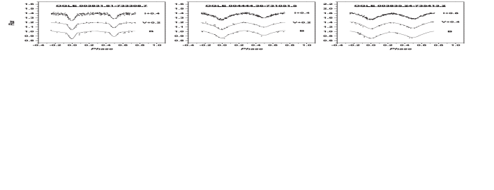
Figure 1: Illustrations of the fit quality of our light curve solutions

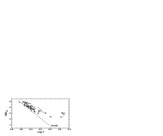
Figure 2: Herzschprung-Russell diagram of SMC stars (the filled and empty symbols refer to the primary and secondary components of the eclipsing binaries, the dotted line presents ZAMS)

5 Conclusion

The eclipsing stars are important sources of information concerning fundamental problems of stellar astrophysics because they allow determination of the global stellar parameters (radii, masses, luminosities, stellar composition). Moreover the investigations of eclipsing binaries in large and homogenous sample give a possibility to improve the empirical statistical relations between these parameters and provide empirical tests for the stellar evolution. This investigation is a small step in the solution of this important problem.

Acknowledgements. The research was supported partly by funds of the project DO 02-362 of Bulgarian Science Foundation.

References

- [1] Alcock C. et al. 1997, AJ 114, 326
- [2] Bouchet P. et al., 1985, A & A 149, 330
- [3] Bradstreet D., Steelman D., 2004, Binary Maker 3 User Manual
- [4] Bronstein V., 1972, Kvant 9, 22
- [5] Dvorak T. Z., 1974, Acta Cosmologica 2, 13
- [6] Flower P., 1996, ApJ 469, 355
- [7] Graczyk D., 2003, MNRAS 342, 447
- [8] Grison P. et al., 1995, A & A 119, 447
- [9] Harries T., Hilditch R., Howarth D, 2003, MNRAS 339, 157
- [10] Hilditch R., Howarth D., Harries T., 2005, MNRAS 357, 304
- [11] Kjurkchieva D., Ivanov V., 2006, BgAJ 8, 57
- [12] Kjurkchieva D., Ivanov V., Rao M., 2007, Annual of Shumen University XVII B2, 44
- [13] Kjurkchieva D., Ivanov V., Radusheva P., Mustafa J., 2008, Annual of Shumen University XVIII B1, 38
- [14] Paczynski B. et al., 1999, arXiv:astro-ph/9908043 v2
- [15] Prsa A., Zwitter T. 2005, ApJ, 628: 426-438
- [16] Udalski A., Kubiak M., Szymanski M. et al., 1997, Acta Astron. 47, 319
- [17] Udalski A., Szymanski M., Kubiak M., 1998, Acta Astron. 48, 147
- [18] Udalski A., Szymanski M., Kubiak M. et al., 2000, Acta Astron. 50, 307
- [19] Wilson R., Devinney E., 1971, ApJ 166, 605
- [20] Wilson R., 1992, Preprint “Documentation of Eclipsing Binary Computer Model”
- [21] Wilson R., Van Hamme W., 2003, Preprint “Computing Binary Star Observables”
- [22] Zaritsky D., Harris J., Thompson I., Grebel E., Massey P., 2002, AJ, 123, 855
- [23] Zebrun K., Soszynski I., Wozniak P., 2001, Acta Astron. 51, 317