Changing approaches of prosecutors towards juvenile repeated sex-offenders:
A Bayesian evaluation

Abstract

Existing state-wide data bases on prosecutors’ decisions about juvenile offenders are important, yet often un-explored resources for understanding changes in patterns of judicial decisions over time. We investigate the extent and nature of change in judicial behavior toward juveniles following the enactment of a new set of mandatory registration policies between 1992 and 1996 via analyzing the data on prosecutors’ decisions of moving forward for youths repeatedly charged with sexual violence in South Carolina. To analyze this longitudinal binary data, we use a random effects logistic regression model via incorporating an unknown change-point year. For convenient physical interpretation, our models allow the proportional odds interpretation of effects of the explanatory variables and the change-point year with and without conditioning on the youth-specific random effects. As a consequence, the effects of the unknown change-point year and other factors can be interpreted as changes in both within youth and population averaged odds of moving forward. Using a Bayesian paradigm, we consider various prior opinions about the unknown year of the change in the pattern of prosecutors’ decision. Based on the available data, we make posteriori conclusions about whether a change-point has occurred between 1992 and 1996 (inclusive), evaluate the degree of confidence about the year of change-point, estimate the magnitude of the effects of the change-point and other factors, and investigate other provocative questions about patterns of prosecutors’ decisions over time.

, , and t1Supported by CDC Grant R49-000-567. t2Supported in part by NIH Grants P20 RR017696-06 and 5U10 DA013727-09.

1 Introduction

In the United States, juvenile sex offenders are increasingly being treated as adult offenders, and are being subjected to similar punishments and restrictions [Letourneau and Miner (2005)]. In particular, federal and state sex offender registration and public notification requirements have been extended now to include juveniles, with little consideration of differences between adult and juvenile development or culpability [Garfinkle (2003)]. Ideally, these considerations should influence legal responses to juvenile criminal behavior [Trivits and Reppucci (2002); Zimring (2004)]. A series of landmark registration laws and policies dealing with juvenile sex offenders was implemented across the US throughout the mid-to-late 1990s [Chaiken (1998)]. Initially, these important policies required probationers and paroled sexual offenders to register personal information with law enforcement (‘registration’ laws), but subsequent major amendments increased public access to registry data (‘notification’ laws).

These policies, including community notification or public registration, were enacted with great hope to improve community safety via either preventing or detecting early recidivism of sexual offenses (e.g., community members can notify the police about suspicious behavior by a known sex offender), as well as deterring sex offenders from committing new sexual offenses (e.g., offenders may be discouraged from committing new offenses if they believe that both the police and community members are providing additional surveillance of their activities) [LaFond (2005); Terry and Furlong (2004)]. The extent of such intended beneficial effects of these registration policies has been questioned [LaFond (2005)] and substantive concerns have been raised regarding possible latent negative consequences of such policies [e.g., Edwards and Hensley (2001); Tewksbury (2005); Zevitz (2006)], particularly with respect to the application of these policies to juvenile offenders [Trivits and Reppucci (2002); Zimring (2004); Chaffin (2008)].

While most studies of latent consequences of such policies have focused on barriers to the successful reintegration of offenders into society [Levenson and Cotter (2005)], it also has been theorized by some that the perceived severity of some registration policies might have the unintended effect of reducing the likelihood of formal prosecution [LaFond (2005)]. One recent survey of family and juvenile court judges reported that the majority of judges believed ‘registration’ could be harmful to juvenile offenders [Bumby, Talbot and Carter (2009)]. Arguably, such a perception of these policies may affect the decisions of prosecutors and judges. We would like to evaluate the strength of the available data evidence to support the hypothesis of judicial decision makers (particularly prosecutors) becoming less likely to prosecute a juvenile charged with sexual offense during the period of enactment of these policies. To address this, we analyze the data on prosecutors’ decision making pattern toward juvenile sexual offense charges during 1988–2005, a period of time encompassing the enactment of sex offender registry and other related laws/amendments in South Carolina (SC). To further understand the extent of the change in decision patterns of the prosecutors, we would also like to estimate the magnitude of this change (if it exists) in terms of change in odds of prosecution after the change-point time and determine other factors affecting the prosecutors’ decisions during this period.

1.1 Prosecution of juvenile sex offenders

We now explain the reasons for focusing on responses from prosecutors for understanding the changes in the judicial decision makers’ actions toward juvenile offenders. After a certain charge has been brought against a youth by law enforcement, the prosecutor is the first judicial decision maker encountered by the youth. Other judicial decision makers such as judges play their respective role only after a prosecutor’s decision to move forward on the case has been made. South Carolina has a very well maintained juvenile justice database which serves as an invaluable resource for examining the change in patterns of prosecutor’s decision-making. We reiterate that we decided to use the prosecutors’ decisions to move forward on initial felony sexual offense cases as the response variable relevant to prosecutors decisions.

Like many other states, SC’s registration and notification policies enacted in 1995 and 1999, respectively (SC Code of Laws $\S\S$ 23-3-400 et seq.) exceed, in every respect, the original federal registration and notification requirements established in the 1990s (e.g., Federal 42 USCA $\S$ 14071, 14072; Pub. L. No. 104-145, 110 Stat. 1345) and continue to exceed even the expanded requirements more recently established by the Adam Walsh Child Safety and Protection Act of 2006. To give some examples of the deviations from federal guidelines, SC’s policies (a) require lifetime registration with no exceptions; (b) have no lower age limit for the registration of sexual offenders (e.g., children as young as 10 years of age have been required to register) and make few distinctions between juvenile and adult offenders; (c) make no distinctions between low and high risk offenders; and (d) include noncontact sexual offenses such as voyeurism and indecent exposure. Due to the breadth and great severity of SC’s policies and their application to teens and pre-teens, it is anticipated that SC’s policies have unintended effects of reducing the probability of prosecutor’s decision of moving forward with the initial sexual charge.

1.2 Focus on repeat sexual offense charges

We have chosen the binary response of prosecutor decision to prosecute (called ‘moving forward’) as the primary response variable related to judicial decision. We investigate the nature and magnitude of changes in probability of moving forward with juvenile sexual offense by studying the available data about an interesting group of 358 male youths charged with sexual offenses in SC at least twice. The effects of public registration policies on repeat offenders have not yet been examined (for both adult or juvenile offenders) but they are relevant for several reasons. First, registration and notification policies were developed in response to public outrage over especially heinous and well-publicized sexual offenses by known sex offenders [LaFond (2005)]. These policies were intended to target only the most severe offenders who were unlikely to be juveniles because sexual recidivism is rare for youth offenders [Fortune and Lambie (2006)]. However, a repeat offense charge might serve as a useful indicator of offender severity. Second, as has been demonstrated in previous research [Howell (2003)], number of prior offenses (any offense, not just sexual) may influence the likelihood of cases moving forward. There was some evidence to suggest that prosecutors may distinguish between first-time and repeat offenders. Whether this finding applies to repeat juvenile sex offenders is unknown. Third, if it is found that the risk of registration negatively influences the likelihood of prosecution even for repeat offenders [as it apparently does for first-time offenders; see Letourneau et al. (2009)], the public policy implications of such a finding would be profound. Juvenile justice encounters for sex crimes contribute little to the prediction of adult sex crimes [Caldwell (2002); Zimring, Piquero and Jennings (2007)]. Nevertheless, repeat juvenile sex offenders represent a small but important subgroup that might benefit from additional surveillance and treatment that accompanies adjudications. Most sexual offenders in the US receive treatment only after legal prosecution and undetected sex offenders have little motivation to seek out professional help. Thus, youths who are not prosecuted for serious sexual offenses are unlikely to receive proper treatment or supervision. Recent evidence of sex offender treatment effectiveness [Letourneau et al. (2009)] makes evidence-based treatment of these youth all the more compelling.

There can be substantial amount of heterogeneity among youth offenders due to how differently they interact with judiciary. This unobservable interaction for each youth will be modeled by a youth-specific random effect. Analyzing data with repeated ($\geq$2 per youth) binary responses of prosecutors’ decisions of moving forward at different time points will allow us to assess the effects of the unobservable prosecutor-youth interaction on prosecutor’s decision. Available data will facilitate the assessment of whether prosecutors treat youths differently during a first offense charge compared to a subsequent charge. Thus, following the change-point year, prosecutors might become more lenient on first time offenders, while at the same time they might adopt a more hardened approach to recidivists.

Figure 1: Panel plots of observed proportion $p$ of prosecutor’s moving forward versus prosecution years. Panel (a): full data, panel (b): repeated offense, panel (c): first-time offense, panel (d): severe offense and panel (e): nonsevere offense.

1.3 Unknown change-point

As noted before, our available data spans from 1988 through 2005. It is conceivable that changes in patterns of prosecution could occur in any one (or more) of these years. Given implementation of South Carolina’s registration policy in 1995, we are most interested in determining whether there is substantial data evidence for 1995 as a change-point year. As seen in the plot of the raw data [Figure 1(a)], there was a high magnitude of decrease in the observed proportion of prosecutors moving forward from 1994 to 1995 and this decrease appears substantial relative to other fluctuations occurring within the full time interval. However, it is difficult and naive to make any conclusion about possible change-point year and magnitude of change in probability of moving forward from these raw proportions (computed via ignoring effect of any covariate). Furthermore, state data on juvenile arrest rates (for rape) also confirm a substantial drop around 1994–1995 [McManus (2005), page 161], suggesting the influence of the 1995 legislation on other judicial actors. Last, our own previous research supports a change in prosecution patterns in 1995 for a data set with predominantly single offense charges [Letourneau et al. (2009)].

There has been almost no research on repeat offenses by juvenile sex offenders and, thus, it is an open argument as to whether the possible change-point year for this smaller subset of offenders should be restricted to a single year, 1995 in particular. The mandatory registration policy enacted in South Carolina in 1995 might not be the main landmark policy for this group. For example, 1996 was the year when several sex crimes were classified as ‘no parole’ crimes as part of South Carolina’s ‘truth in sentencing’ policies. Likewise, changes in juvenile transfer policies that made it easier to transfer younger defendants (14–15 years old) to adult court for certain offenses also occurred in 1996. Thus, these or other policy or policy changes (e.g., lengthened sentences) could exert influence on the pattern of juvenile judicial decision making. In spite of using our apriori belief that the most likely year for change is 1995, our discrete prior distribution of the unknown change-point year in between 1992 and 1996 will reflect a skeptical view that laws enacted in years other than 1995 might also have caused the change in pattern of prosecutors’ decisions. It could also be argued that legal policies take time to reach their full effect on decision makers (e.g., reflecting a learning curve among judicial decision makers regarding the severity of a policy) and that focusing on a single year of sudden change-point is unnecessarily narrow. To address this concern, we incorporate a linear and a quadratic coefficient of change-point effect to provide the flexibility of the nature of effects generated by the change-point (if it exits).

If we find credible data evidence for any change in prosecutor’s pattern of moving forward during 1992–1996, we would further like to find out the most likely year of change-point as well as the magnitude of the change in terms of odds ratio before and after the change-point year. The actual magnitude of the change-point effect is important to understand the practical consequences to society for such a change. We will handle these complex goals using a model for longitudinal binary data where the change in the odds of going forward after the change-point year can be estimated. Our model is very different from the unknown change-point model used for single time-series of quantitative responses discussed in Carlin and Louis (2000) and other related works.

1.4 Youth heterogeneity and conditional/marginal odds ratio

Large sample based analysis using generalized estimating equations (GEE) for multivariate clustered binary outcomes [Zeger and Liang (1986)] is very common in biomedical and behavioral studies. However, the unobservable prosecutors’ reaction to different individual youths (youth specific youth-prosecutors interaction effect) can substantially attenuate the actual subject-specific effects of covariates and time/year and change-point on the pattern of judicial decision making. The marginal GEE approach is unable to estimate this degree of attenuation. This attenuation is a measure of variability among youths regarding some youths being more predisposed (compared to others) to receive a moving forward decision.

In our analysis, we express this latent/unobservable youth-specific interaction as a random youth effect. We are interested in determining the amount of attenuation in the effects of the change-point year and would like to make probability statements about the actual change in probability of moving forward in a particular year (say, 1995) based on observed data. Consequently, we want to maintain key advantages of a marginal model based GEE approach such as simple physical interpretation of covariates and change-point year effects in terms of the marginal odds ratio. To achieve this goal, we present an extension of the random intercept model proposed by Wang and Louis (2003) in which the subject-specific model (conditional on the youth-specific random intercept) as well as the marginal model (integrated over the distribution of the unobservable random intercept) have the same link functions. The regression parameters in our conditional and marginal models are not identical, but are proportional to each other and the proportionality parameter will represent the attenuation of all the covariate and change-point effects on marginal response due to heterogeneity of youths. For example, consider a youth with two offenses committed before and after the change-point year. Our model will be able to assess the individualized odds of moving forward for the offense before change-point year and the odds of moving forward for the same youth’s offense committed after the change-point year. The model will also be able to assess the marginal odds ratio of moving forward for two offenses committed by two different youths. This marginal odds ratio is smaller than the corresponding conditional/individualized odds ratio.

2 Brief overview of the data

Every South Carolina youth (male) charged by the Department of Juvenile Justice (DJJ) with repeated felony-level sexual offenses between January 1, 1988 and December 31, 2005 is included for the present analysis. Female offenders were excluded due to the small number of females in the database. Charges filed against minors in general sessions (adult court) were not included in the study. The analysis focused on felony sexual offenses because South Carolina’s registration and notification policies primarily apply to sexual offenses. All data were drawn from the South Carolina DJJ Management Information System in collaboration with the South Carolina Budget and Control Board Office of Research and Statistics. The data included a subset of variables regularly captured by DJJ personnel during processing of each charge and subsequently during progression of the case, viz. (a) demographic information, (b) youth’s criminal history, and (c) information regarding specific sexual felony charge (viz. type of charge, degree of severity, charge date, prosecutor’s decision, etc.).

The database included records for 358 male offenders with a total of 753 offenses. For each charge, the prosecutor decision could indicate moving forward (i.e., decision to formally adjudicate the youth), diversion (i.e., decision to refer youth to a nonjudicial intervention that, if successfully completed, would clear the initial charge), or dismissal (i.e., decision to not process or otherwise dismiss the case). The longitudinal response variable $Y_{it}$ for youth $i$ at calendar time $t$ is the binary indicator with $Y_{it}=1$ for moving forward (70.7% of cases) and $Y_{it}=0$ for diversion or dismissal of the charge by the prosecutors (29.3% of cases).

For each youth, a set of known/observable explanatory variables (fixed or time-dependent) were recorded that may influence the probability of prosecutor’s going forward. The set of fixed explanatory variables include age at the time $t$ of the offense, an indicator of repeated offense, severity index of the offense, prosecution year, etc. The median age for this group of male youths was 14.6 years with a range of 9–19 years. The charge severity rating for each felony sexual charge determined by DJJ is based on the number of years an adult would be incarcerated for a similar crime. The charge severity ratings range from 1 (lowest level misdemeanor) to 25 (highest level felony and typically reserved for 1st degree murder charges), with felony offenses operationally defined as charges with severity ratings of 5 or higher [Barrett, Katsiyanis and Zhang (2006)]. In practice, felony level sex crimes had severity ratings of 5, 8, 15 and 21. For simplicity, we use a binary indicator to classify the severity rating as severe (80.5% cases with severity rating $>$ 8) and nonsevere (19.5% cases with severity rating $\leq$ 8). Similarly, we use a binary indicator to record whether a particular offense is a repeated offense. Out of the total 753 felony level sex offenses, 395 (52.4%) were repeated offenses and the rest 358 (47.6%) were the first-time offenses. Table 1 shows the $2\times 2$ table for the actual counts and proportions for charges with two severity levels versus first-time/repeat charges.

Table 1: $2\times 2$ table showing frequencies of repeat/first-time offenses vs. severe/nonsevere offenses

	Severe offense	Nonsevere offense	Total
Repeated offense	284 (38%)	111 (15%)	395
First-time offense	322 (43%)	036 (4%)0	358
Total	606 (43%)	147 (43%)	753

There were 481 cases (63.8%) of prosecution conducted after the registration policy was implemented in January 1995. Of the 358 male offenders, 326 (91.1% cases) had 2 offenses. Among the remaining 32 youth offenders, 28 (7.8% cases) had 3 offenses, 3 (0.83% cases) had 4 offenses and 1 (0.27% cases) had 5 offenses. Thus, each offender represents a cluster with the maximum cluster size being 5. Figure 1 shows panel plots of the raw proportion of prosecutors moving forward vs. year of prosecution for all charges (panel a), charges for repeated offenses (panel b), charges for first-time offenses (panel c), charges for severe offenses (panel d) as well as charges for nonsevere offenses (panel e). The figure suggests some possible effect around 1995; however, the actual year of change-point and its association with the type of charge (severe/first-time/repeat) are not clear from the plots. The evidence of a latent change-point between 1992 and 1996 and its magnitude of influence on prosecutors’ decision and other conjectures about the pattern of decisions over time can only be evaluated with a semi-continuous (change-point) model along with linear and quadratic effects of change-point (that determines whether this change effect was gradual over years). Any interaction of each known explanatory covariate with the change-point indicator (viz. repeat offense indicator with change-point indicator) will be considered as a time-dependent covariate. In the year 1999, the sexual offender registry became available online and about half of registered juveniles were included. In addition to the unknown change-point effect, we will also attempt to verify whether the notification law of 1999 influenced the prosecutor’s decision since the year 2000. There are 252 cases (33.5%) of prosecution after the implementation of the online registry in 1999. Out of our concern for statistical association between different pairs of explanatory variables (after properly accounting for clustering), we used the non-Bayesian Rao–Scott chi-square test (available in SAS Procedure SURVEYFREQ) to find strong evidence of association between the repeat offense indicator and the severity indicator ($p$-value $<$ 0.001). We did not expect any association among all other variables and similar frequentist tests for evaluating association between the remaining explanatory variables are not statistically significant. In our formal Bayesian analysis, we will evaluate whether both severity indicator and repeat offense indicator should be included simultaneously as predictors.

The time-interval of the study (1988–2005) permitted examination of cases processed during years prior to implementation of the South Carolina sex offender registration (i.e., January 1, 1988–December 31, 1994), as well as cases processed during the four years following registration but prior to implementation of the online registry website (i.e., January 1, 1995–December 31, 1998) and cases processed during the years subsequent to implementation of the Internet-based public registration (i.e., January 1, 1999–December 31, 2005). One of our aims in this article is to draw statisticians’ attention to this important class of databases. These data can be extensively and critically modeled and analyzed to investigate whether our judicial decision making process is changing with time, with ever-shifting societal perception and evolving legislative activism. Assessing the existence and effect of the change-point time induced by mandatory registration laws on the prosecutor’s decision of moving forward with a juvenile sex offense case has tremendous societal implications in its own right and hence demands serious exploration of available evidence via these databases.

3 Bridge random effects model

Our modeling goal is to interpret the effects of change-point and other factors on the changes in ‘odds of moving forward’ for a particular charge. The following model using a particular random effects density (called the ‘Bridge’ density) preserves the odds ratio interpretation of the change-point and other factors.

For $i=1,\ldots,n$ exchangeable youths/subjects, sexual charges were brought against youth $i$ at years $t=t_{i1},\ldots,t_{im_{i}}$ for $m_{i}\geq 2$. The binary response of interest is $Y_{it}=1$ if the prosecutor decides to move forward (proceed with the prosecution) for the sexual offense charge against the youth $i$ at time $t$, and $Y_{it}=0$ otherwise. For the random effects logistic regression model, the conditional probability $p_{it}(B_{i})=\operatorname{pr}[Y_{it}=1|B_{i},\underline{x_{it}}]$, given the subject-specific unobservable $B_{i}$ and the known $p\times 1$ covariate vector $\underline{x_{it}}$ measured at time $t$, is

$$p_{it}=\frac{\exp(B_{i}+\bolds{\beta}\underline{x_{it}^{\prime}})}{1+\exp(B_{i}+\bolds{\beta}\underline{x_{it}^{\prime}})},$$ (1)

where $\bolds{\beta}=(\beta_{1},\ldots,\beta_{p})$ denotes the vector of regression parameters. The offender-specific unobservable random effects $B_{i}$ has density $f_{B}(b|\phi)$ with the variability parameter $\phi$. The binary model with logit link in (1) gives an easily understandable proportional odds interpretation of the covariate effects when we know the unobservable youth-specific $B_{i}$. However, the change in odds ratio interpretation of the regression effects is not preserved in general after integrating out $B_{i}$. When $B_{i}$ follows a bridge distribution of Wang and Louis (2003) with density,

$$f_{B}(b|\phi)=\frac{1}{2\pi}\frac{\sin(\phi\pi)}{\cosh(\phi b)+\cos(\phi\pi)},\qquad-\infty<b<\infty,$$ (2)

indexed by unknown parameter $0<\phi<1$, the marginal probability of moving forward (after integrating unobservable youth-specific $B_{i}$), still preserves the logistic form unlike normal and $t$-density random effects and is given as

$$\operatorname{Pr}(Y_{it}=1|\underline{x_{it}})=E_{B}[p_{it}(B_{i})]=\frac{\exp[(\phi\bolds{\beta})\underline{x_{it}^{\prime}}]}{1+\exp[(\phi\bolds{\beta})\underline{x_{it}^{\prime}}]},$$ (3)

where $E_{B}$ denotes the expectation with respect to the density of $B_{i}$.

Figure 2: Probability density functions of Bridge, Normal and $t$-densities with zero mean and variance $=$2. The $x$-axis denotes the range of $x$-values from $-$5 to 5.

The bridge density is symmetric around mean zero [Wang and Louis (2003)] with the variance given by $\sigma_{B}^{2}=\pi^{2}(\phi^{-2}-1)/3$. Figure 2 displays the comparison of the bridge density (with variance $=$ 2) with a $\operatorname{Normal}(0,\sigma^{2}=2)$ and a $t$-density having degrees of freedom $\nu=4$ (corresponding to a variance of 2). The bridge density has a slightly heavier tail and is more peaked than the normal and the $t$-densities. We again emphasize that, unlike the normal and the $t$-density, both the conditional probability in (1) and the marginal probability in (3) of moving forward under the bridge density random-effects have logistic links, with proportional odds interpretations of the regression effects.

Figure 3: LOWESS smoothed plots of observed proportion of moving forward vs. estimated (mean) proportion of moving forward for pre-95 and post-95 years.

To assess the need of incorporating a change-point structure into our logistic regression framework, we divided the whole data into two sections, (i) prosecution year $<$ 1995 and (ii) prosecution year $\geq$ 1995, and fit separate logistic regression models (using PROC LOGISTIC) in SAS, considering all data points to be independent in each of the models. We used prosecution age, severity indicator, repeat offense indicator and prosecution year as covariates without any change-point term. Then, the observed proportion of prosecutors ‘moving forward’ versus the estimated (mean) proportion of prosecutors ‘moving forward’ (after LOWESS smoothing) were plotted in Figure 3, overlayed on each other. The simple logistic model for the ‘post-95’ data is clearly inadequate, as expected, due to the effect of the change-point somewhere around 1995. Clearly, there is a need to account for the (possibly unknown) change-point structure in our model. The Bayesian paradigm allows us to use effectively our apriori belief about the occurrence of the change-point.

In this article we will use a novel extension of the longitudinal binary model of (1) by allowing time-dependent covariates $\underline{x_{it}}(T)$ which are functions of unknown year of change-point $T$ as well as calendar time $t$. To incorporate the effects of an unknown change-point year $(1992\leq T\leq 1996)$, the covariate vector has two components, viz. (a) a vector $\underline{x_{1it}}$ of either fixed or time-dependent known/recorded covariates such as age at charge, binary indicator of repeat offense for the charge, a dichotomized indicator for severity of offense, an indicator for the year of notification ‘2000,’ the prosecution year $t$, and (b) a vector $\underline{x_{2i}}(t,T)$ of known functions of prosecution year $t$ and unknown change-point year $T$ common to all subjects. The functions of unknown $T$ include the change-point indicator $1_{[t\geq T]}$, a linear coefficient of the change-point indicator $(t-T)1_{[t\geq T]}$ and also a quadratic coefficient $(t-T)^{2}1_{[t\geq T]}$. The change-point term $1_{[t\geq T]}$ accommodates a sudden change in the pattern at time $T$. The linear and quadratic terms allow the change in pattern to be continuous after the unknown change-point year $T$. We will later discuss how to use discrete prior distribution of $T$ to reflect our prior opinion about what value/year $T$ can take in the interval 1992–1996. We also include the interaction of ‘repeat offense’ and ‘change-point indicator’ $1_{[t\geq T;\mathit{Repoff}=1]}$ to assess whether the magnitude of the change in prosecutors’ decision pattern after $T$ depends on whether the charge is a first time offense versus a repeat offense.

Our extension of the model in (1) is given as

$$\operatorname{logit}\{p_{it}(B_{i},T)\}=B_{i}+\bolds{\beta_{1}}\underline{x^{\prime}_{1it}}+\bolds{\beta_{2}}\underline{x^{\prime}_{2i}}(t,T),$$ (4)

where the vectors $\bolds{\beta_{1}}$ and $\bolds{\beta_{2}}$ represent respectively the regression parameters associated with the observable fixed/time-dependent covariates and the effect of the unknown change-point $T$ at year $t$. Using our model, we can interpret the effect of each covariate, because we can obtain the marginal as well as the conditional odds ratio. For example, if we define the parameter for the indicator of repeat offense to be $\beta_{\mathit{Repoff}}$, then the conditional odds ratio $e^{(\beta_{\mathit{Repoff}})}$ represents the ratio of the odd of moving forward when an individual is charged with a repeat offense and the odd of moving forward when the same charge is for a first offense. The attenuated marginal odds ratio $e^{(\phi\beta_{\mathit{Repoff}})}$ measures the ratio of the odd of moving forward for a youth charged with repeat offense and the odd for another similar youth charged with a first offense. The variability parameter $0<\phi<1$ of the bridge density measures both the degree of attenuation of the marginal/population effect versus conditional/individualized effect and the heterogeneity of the decision making process. The extreme case of $\phi=1$ represents the situation when there is no effect of the unobservable youth-prosecutor interaction and the responses corresponding to all the charges from all the youths can be considered as exchangeable. The extreme case of $\phi=0$ represents the situation when the unobservable youth-prosecutor effect is so high that it alone determines the decision of moving forward. Unless we get strong data evidence against the bridge density for $f_{B}(\cdot|\phi)$, we will prefer using the model defined by (1) and (2) because this model ensures the convenient proportional odds interpretation of the effects of covariates and change-points both conditionally and marginally, and offers a simple role of the heterogeneity parameter $\phi$ as the attenuation factor of the marginal odds ratio of two subjects in the presence of heterogeneity.

Using the regression model of (4), we can write the likelihood of $\bolds{\beta}$, the unknown $T$ and the random effects $\mathbf{B}=(B_{1},\ldots,B_{n})$ based on the observed data $\mathbf{y}$ as

$$L(\bolds{\beta},\mathbf{B},T|\mathbf{y})\propto\prod_{i=1}^{n}\prod_{j=1}^{m_{i}}\{p_{it_{ij}}(B_{i},T)\}^{y_{it_{ij}}}\{1-p_{it_{ij}}(B_{i},T)\}^{y_{it_{ij}}}.$$ (5)

To draw conclusions about the effects of covariates and the unknown change-point year on the odds of moving forward, we used a Bayesian analysis of the random effects logistic regression model accommodating unknown change-point time $T$. The posterior conclusion for a Bayesian analysis is based on the joint posterior of all the parameters given by

$$p(\bolds{\beta},\mathbf{B},T,\phi|\mathbf{y}) \propto L(\bolds{\beta},\mathbf{B},T|\mathbf{y})$$

$${}\times\Biggl{[}\prod_{i=1}^{n}f_{B}(B_{i}|\phi)\Biggr{]}\times\pi_{1}(T)\times\pi_{2}(\bolds{\beta})\times\pi_{3}(\phi),$$

where $\pi_{1}(T)$, $\pi_{2}(\bolds{\beta})$ and $\pi_{3}(\phi)$ are independent priors of $T$, $\bolds{\beta}$ and $\phi$ of the bridge density $f_{B}(B_{i}|\phi)$ of (2). The key advantage of relying on Bayesian inference to address the pertinent question of the influence of the sex-offender registration laws on prosecutor’s decision making is the ability to incorporate background (prior) information about the unknown parameters including the unknown change-point year $T$. Thus, a proper selection of prior information is an important step toward making an informed conclusion about the data evidence from the study. Unlike the frequentist inference depending on large-sample inference, the Bayesian method relies heavily on the simulations from the posterior of (3) via the Gibbs sampler [Gelfand and Smith (1990)] and associated Markov chain Monte Carlo (MCMC) tools. The MCMC method provides the entire posterior distribution of any arbitrary functional of the parameters. In the following section we discuss the determination of practical prior distributions for $\phi$, discrete time $T$ and regression parameter $\bolds{\beta}$.

4 Choice of priors

In this section we develop practical informative prior distributions for the parameters including the attenuation parameter $\phi$ and the unknown change-point year $T$. While selecting a prior density class/model, we prefer a class of densities with a small set of informative features to be selected by investigators/statisticians. For each component $\beta_{k}$ for $k=1,\ldots,p$ of the regression parameter $\bolds{\beta}$, we use the zero centered double exponential (DE) prior (often called Laplace prior) $\beta\sim\operatorname{DE}(0,\tau)$, with p.d.f. $\frac{\tau}{2}\exp(-\tau|\beta|)$ for $-\infty<\beta<\infty$, and variance $2/\tau^{2}$. The DE prior is a widely used sparsity inducing prior with a heavy tail and peakedness at 0, and hence expressing the prior belief that the distribution of $\beta_{k},k=1,\ldots,p$ is strongly peaked around 0 [Kaban (2007)]. This prior reflects our ‘skeptical’ views about the covariate and change-point effects. Our strategy is to hold such a skeptical prior view unless there is a strong data-evidence suggesting otherwise. We choose the precision parameter $\tau=\sqrt{2}$ for each $\beta_{k}$. This choice of $\tau$ makes the prior variance of $\beta_{k}$ to be one. Assuming $\beta_{k}=1$ and a logistic model with a single covariate, this corresponds to a prior belief that a change in 1 unit of a covariate can change the value of probability $p_{it}$ of going forward from 0.5 to 0.73. For this data example, we believe our prior belief allows for a large enough effect of each covariate (keeping other covariates fixed) because 23% change in $p_{it}$ for a unit change of a covariate is a very large change to expect in practice.

Our first prior for $\phi$ also represents a ‘skeptical’ (however, informative) opinion that heterogeneity among young offenders does not cause large attenuation of regression effect in marginal probability of moving forward. To assure this, a $\operatorname{Beta}(2,1)$ prior density (with mean 0.67) is chosen for $\phi$ to make the prior skewed toward 1. As an alternative, a $\operatorname{Beta}(1,1)$ [the $\operatorname{Uniform}(0,1)$ prior] is considered as a competing ‘noninformative’ benchmark prior for $\phi$.

We believe that the change-point year is within the interval 1992–1996 (if the change-point had taken place at all), with the most plausible year being 1995. We use a Dirichlet prior on the years 1992–1996, that is, $(\gamma_{92},\ldots,\gamma_{96})\sim\operatorname{Dir}(\alpha_{92},\ldots,\alpha_{96}),$ with joint density $\pi(\gamma_{92},\ldots,\gamma_{96})\propto\prod_{j=92}^{96}\gamma_{j}^{\alpha_{j}}$, where $\gamma_{j}=\mathrm{P}[T=j]$ and prior expectation of $\gamma_{j}$ equals $\alpha_{j}/\alpha_{+}$ with $\alpha_{+}=\sum_{j=92}^{96}\alpha_{j}$. We provide more prior weight to 1995 (landmark registration year) being the unknown $T$ compared to the other years. A prior belief very enthusiastically favoring 1995 as $T$ is given by (a) $(\alpha_{92},\ldots,\alpha_{96})=(1,1,1,6,1)$. This prior implies the expected prior probability that the change-point happened in 1995 is 0.6, and the rest of the years in 1992–1996 has equal prior probability. To represent a more skeptical belief, we consider two more choices of the Dirichlet parameters, viz. (b) (1.6, 1.6, 1.6, 5, 1.6) representing an expected prior probability of 0.45 for $T=1995$ and 0.14 for each of the other years and (c) (1.5, 1.5, 1.5, 3, 1.5) representing an expected prior probability of 0.33 for $T=1995$ and 0.167 for the other years. It is important to note that the prior in (b) has higher $\alpha_{+}$ than (a) and (c). This implies that the certainty about the value of each $\gamma_{j}$ is higher in (b) compared to the other priors.

For a better description of the practical implication of our prior densities, we also determine the extent of the effect of each component of $x_{it}$ on the ‘change in odds of moving forward’ as expected by our prior choice. We recall that the marginal prior density of each component $\beta_{k}$ is assumed to be identical here. Based on two prior choices of $\phi$, that is, $\phi\sim$ $\operatorname{Uniform}(0,1)$ and $\phi\sim\operatorname{Beta}(2,1)$, the change in odds of moving forward can be anywhere between 0.05 and 14.4 with 95% probability. This shows that our particular joint priors allow for the possibility of a very large change in odds of moving forward in either direction. To address a practical concern about whether each of our prior models allow wide flexibility about the probability of moving forward at any particular year, we verified whether the range of possible values of the probability

$$p^{*}_{T,t}=\frac{\exp(\phi\bolds{\beta}\underline{x^{*}}^{\prime}(t,T))}{1+\exp(\phi\bolds{\beta}\underline{x^{*}}^{\prime}(t,T))}$$ (7)

are wide enough for all possible values of $t$ and $T$. We consider $p^{*}_{T,t}$ as the probability of moving forward for a randomly selected youth (with median age) charged with a severe repeat sexual offense in year $t$ when the change-point year $T$ is known. For $t=1996$ and $T=1995$, the range between 0.004 and 0.997 indicates that our prior belief allows a wide range of possible values of the probability of moving forward at any year.

5 Bayesian computation and model selection

In this section we discuss the MCMC computation and model selection and assessment procedures for eight competing models, determined by the sets of prior assumptions for change-point $T$ and the attenuation parameter $\phi$. The reader less interested about technical details about model selection and MCMC computation can skip this section and proceed to the next section for detailed analysis and findings from the study. The competing models under consideration are as follows:

$(\gamma_{92},\ldots,\gamma_{96})\sim$ Dir$(1,1,1,6,1)$ and $\phi\sim\operatorname{Uniform}(0,1)$;

$(\gamma_{92},\ldots,\gamma_{96})\sim$ Dir$(1.6,1.6,1.6,5,1.6)$ and $\phi\sim\operatorname{Uniform}(0,1)$;

$(\gamma_{92},\ldots,\gamma_{96})\sim$ Dir$(1.5,1.5,1.5,3,1.5)$ and $\phi\sim\operatorname{Uniform}(0,1)$;

$(\gamma_{92},\ldots,\gamma_{96})\sim$ Dir$(1,1,1,6,1)$ and $\phi\sim\operatorname{Beta}(2,1)$;

$(\gamma_{92},\ldots,\gamma_{96})\sim$ Dir$(1.6,1.6,1.6,5,1.6)$ and $\phi\sim\operatorname{Beta}(2,1)$;

$(\gamma_{92},\ldots,\gamma_{96})\sim$ Dir$(1.5,1.5,1.5,3,1.5)$ and $\phi\sim\operatorname{Beta}(2,1)$;

model with no change-point;

model with the change-point year fixed at 1995.

The prior for the regression parameters is the same for each of the above prior models. For each prior model representing different prior opinion, the computation of the posterior distribution was performed via iterative MCMC [Gelfand and Smith (1990)] techniques. To sample from the joint posterior under each prior model, we need to sample from the conditional distributions of different model parameters. Each conditional posterior is proportional to the joint posterior density (6) as a function of the corresponding parameter. The conditional posteriors of $B_{i},\bolds{\beta}$ and $\phi$ are log-concave (proofs omitted), therefore, standard adaptive rejection algorithms of Gilks and Wild (1992) are applicable to sample from these conditional posteriors. The relevant Gibbs sampling steps were implemented readily using freeware package $\tt{WinBUGS}$ [Spiegelhalter et al. (2005)]. We used 50,000 iterations with an initial burn-in of 45,000. Convergence of the generated samples was assessed using standard tools such as trace plots and ACF plots as well as Gelman–Rubin diagnostics. The initial values for the fixed effects parameters were selected arbitrarily. We used two different MCMC chains (with two different initial values) to be reasonably confident about convergence. Derivation of the full conditional posterior distributions of model parameters along with associated $\tt{WinBUGS}$ code to implement the estimation strategy is provided in the supplemental article [Bandyopadhyay (2009)].

Our initial model selection was performed using the Deviance Information Criterion (DIC) of Spiegelhalter et al. (2002). DIC reflects the goodness of fit as well as the complexity of the hierarchical model within the Bayesian paradigm and is considered to be a Bayesian version of the Akaike Information Criterion (AIC). It is defined as $\mathit{DIC}=\overline{D}+p_{D}$, where $\overline{D}=E(D(\bolds{\Theta})|\mathbf{y})$ is the posterior mean of the deviance and $p_{D}$ is the effective number of parameters in the model. Spiegelhalter et al. (2002) showed that $p_{D}$ can be approximated as $p_{D}=\overline{D}-D(\hat{\bolds{\Theta}})$, where $\hat{\bolds{\Theta}}$ is a suitable ‘plug-in’ estimate of $\bolds{\Theta}$, viz. the posterior mean, or median. The DIC is essentially a single-number summary (lower is better) of the relative fit between the model and the ‘true model’ generating the data for the purpose of prediction. A difference larger than 10 is considered overwhelming evidence in favor of the better model [Burnham and Anderson (2002)].

After selecting the best model using DIC criterion, we also employed model validation diagnostics through conditional predictive ordinate (CPO) statistics [Gelfand, Dey and Chang (1992)] and the associated ‘log pseudo-marginal likelihood’ (LPML). The CPO is a cross-validated approach and based on posterior predictive probability of observed data. For the observed response $y_{ij}$ from youth $i$ at time $t_{ij}$ with covariate vector $\mathbf{X}_{ij}$, the CPO statistic for observation $(i,j)$ is defined as $\mathrm{CPO}_{ij}=f(y_{ij}|{\mathbf{D}}_{(-ij)})=\int f(y_{ij}|\bolds{\Theta},\mathbf{X}_{ij})\pi({\bolds{\Theta}}|{\mathbf{D}}_{(-ij)})\,d{\bolds{\Theta}}$, where $\pi({\bolds{\Theta}}|{\mathbf{D}}_{(-ij)})$ is the posterior density of parameter vector ${\bolds{\Theta}}$ given ${\mathbf{D}}_{(-ij)}$, the cross-validated data without the $(i,j)$th observation. Using a harmonic mean approximation result fromGelfand, Dey and Chang (1992), the $\mathrm{CPO}_{ij}$ can be easily computed with MCMC samples from the full posterior $\pi(\bolds{\Theta}|\mathbf{D})$. Typically, the $\mathrm{CPO}_{ij}$’s behave as Bayesian residuals and are plotted against any covariate values $x_{ij}$ (or observed $Y_{ij}$’s) to determine patterns of covariate dependence as well as identify possible outliers. Larger values of $\mathrm{CPO}_{ij}$ indicate better support for the model from the observation $y_{ij}$. A summary measure based on the CPO is the logarithm of the psuedo-marginal likelihood (LPML) defined as $\mathrm{LPML}=\sum_{i,j}\log(\mathrm{CPO}_{ij})$, where a higher value of the LPML means better support of the model from the observed data.

We observe that Models 1–6 exhibit somewhat similar fit (based on $\overline{D}$), but the effective parameter count $p_{D}$ greatly varies. Based on the DIC values, we make a more detailed comparison between Models 1 and 5 whose DIC values are the lowest, being 821.4 and 832.3 respectively. For these two models, the DIC scores reflect a considerable trade-off between data fidelity $(\overline{D})$ and the effective number of parameters $p_{D}$. The $p_{D}$ value is much lower for Model 1 ($=$63.4) than Model 5 ($=$76.6). The DIC value for Model 8 (fixed change-point model) was somewhat closer ($=$838.8) to Model 5, but for Model 7 (no change-point model), it was far away ($=$890.6). As described earlier in Section 2, a non-Bayesian but convenient procedure such as the Rao–Scott chi-square test shows a high evidence of association between the binary indicator of repeat offense and the dichotomized severity indicator ($p$-value $<$ 0.001). If we omit the binary severe offense indicator from Model 1, the corresponding interval estimate of the repeat offense indicator has a slightly tighter 95% credible interval ($-$1.041, $-$0.105) than Model 1 at expense of a high DIC price (859.7).

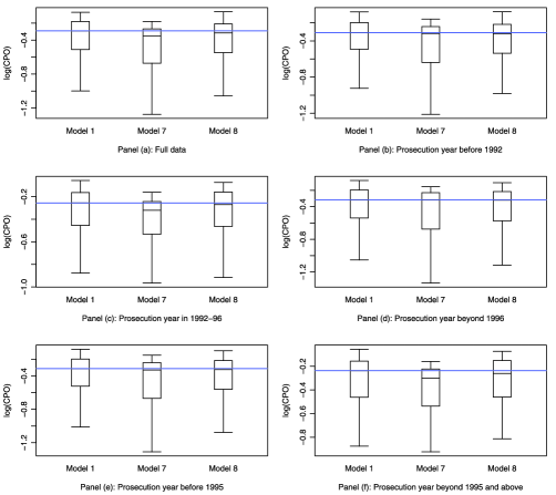
Figure 4: Panel box-plots of $\log(\mathrm{CPO})$ for Models 1, 7 and 8 considering different time intervals of prosecution. Larger values of $\log(\mathrm{CPO})$ indicate more support for the model. The horizontal line in each panel denotes the median $\log(\mathrm{CPO})$ value for Model 1.

To assess model validation in terms of predictive performance, we use the box-plots of $\log(\mathrm{CPO})$ statistics to compare between Models 1, 7 and 8 in Figure 4. The median value of $\log(\mathrm{CPO})$ for Model 1 is indicated by the horizontal line in each of the panels. Panel (a) reveals that on the overall, both Models 1 and 8 (model with fixed change-point) exhibit significantly better predictive performance over Model 7 (model with no change-point), though Model 1 performs marginally better than Model 8. All 3 models have similar fit for prosecution years before 1992 [panel (b)] as well as beyond 1996 [panel (d)]. For the prosecution years between 1992 and 1996 [panel (c)], the $\log(\mathrm{CPO})$ values for Model 1 are marginally better than Model 8 and distinctly better than Model 7. Considering panels (c), (e) and (f), it is clear that there is strong evidence for a model with a change-point around 1995. This is clearly demonstrated in $\log(\mathrm{CPO})$ plots for Models 1 and 8 which includes a change-point term. The LPML values for Models 1, 7 and 8 are respectively $-309.78,-350.72$ and $-320.43$, confirming again a marginally better predictive performance of the unknown change-point model over the fixed change-point model. While Model 1 includes a moderate ‘prior opinion’ of 1995 as the change-point year, Model 8 uses the prior view that the change-point is known to be exactly 1995. Model 1 does not prove to be much superior than Model 8 as determined by DIC and predictive performances, yet we choose Model 1 for further analysis primarily because of the absence of a common mandate in the literature (before this analysis) of restricting 1995 as the change-point year for this subset of juvenile sex offenders with repeated sex offenses.

To determine an overall goodness of fit of Model 1, we also computed the Bayesian $p$-value [Gelman et al. (2004)], which measures the discrepancy between the data and the model by comparing a summary $\chi^{2}$ statistic of the posterior predictive distribution to the true distribution of the data. The summary statistics from the predicted and observed data are given by $\chi^{2}(\mathbf{Y},\Theta^{g})$ and $\chi^{2}(\mathbf{Y}^{\mathit{rep},g},\Theta^{g})$, respectively, where $\mathbf{Y}^{\mathit{rep},g}$ denote the replicated value of $Y$ from the posterior predictive distribution of $\Theta$ at the $g$th iteration of the Gibbs sampler. The Bayesian $p$-value was then calculated as $P(\chi^{2}(\mathbf{Y}^{\mathit{rep},g},\Theta^{g})>\chi^{2}(\mathbf{Y},\Theta^{g}))$, that is, the proportion of times $\chi^{2}(\mathbf{Y}^{\mathit{rep},g},\Theta^{g})$ exceeds $\chi^{2}(\mathbf{Y},\Theta^{g})$ out of $g=1,\ldots,G$ simulated draws from the posterior predictive distribution. For Model 1, we obtain the$p$-value to be 0.41 which indicates an overall reasonable fit, that is, the observed pattern would likely be seen in replications of the data under the true model.

6 Results

Our conclusions of the data analysis were primarily based on Model  1, which is the best model supported by the data. This model uses the apriori belief that the most likely year of change in judicial decision pattern is 1995, however, with a noninformative prior belief about the effect of the change-point as well as the attenuation parameter $\phi$. Based on 95% credible intervals, we found strong posterior evidence of the effects of several covariates on the odds of moving forward which includes (a) age at charge, (b) dichotomized severity of offense, (c) year of prosecution, (d) indicator of repeat offense, (e) indicator of whether the time of offense is after the change-point and (f) interaction between repeat offense and change-point. In particular, prosecutors were less likely to move forward on repeated offense than the first-time sex offenses and less likely to move forward after the change-point. The strong posterior evidence of the positive interaction effect between repeat offense and change-point confirms the need to present the effects of repeat offense charges separately for the time intervals before and after the change-point.

Table 2: Posterior summaries of marginal odds ratios for Model 1. $T$ denotes unknown time of change-point

Odds ratio	Mean	Standard deviation	95% credible intervals
Age	1.150	0.037	(1.094, 1.236)
Repeat offense before $T$	0.604	0.163	(0.308, 0.932)
Repeat offense after $T$	1.131	0.217	(1.014, 1.639)
Severe offense	1.506	0.280	(1.049, 2.132)
Year of prosecution	1.155	0.096	(1.006, 1.373)
After change-point effect	0.256	0.086	(0.132, 0.483)

Table 2 presents the posterior estimates together with 95% credibility intervals (CI) of ‘marginal odds ratio’ of the covariates found to be relevant for the prosecutor’s decision. The marginal odds ratio for any particular factor represents the odds ratio between two randomly selected comparable youths with only a unit difference in the relevant covariate. We now summarize the implications of our results. The prosecutors are about 15% more likely to move forward on charges for every year increase in age, about 16% more likely to move forward for every year increase in prosecution year. The mean increase in probability of moving forward is around 51% for severe offenses as compared to nonsevere offenses. The odds of prosecution of a charge after the change-point year will have a 26% reduction as compared to a charge that happened before the change-point. Overall, prosecutors were less likely to move forward on repeat offense cases. However, compared to a repeat offense charge before the change-point, there is about a 13% increase in the odds of moving forward for a comparable repeat offense after the change-point. Interestingly, the magnitude of this increase in odds may be as low as 1.4%. The posterior probability that the change-point occurred in 1995 (maybe due to the registration policy) for Model 1 is about 61% (95% CI between 32% and 87%), suggesting strong posterior evidence for 1995 being the ‘likely’ change-point year compared to any other year between 1992 and 1996. Interestingly, even for the Models 3 and 6 which use the skeptical prior (c) defined in Section 4, we find similar strong evidence that a change-point has occurred in the interval 1992–1996 (results omitted for brevity). In summary, we conclude that there is strong posterior evidence of the existence of a change-point in between 1992 and 1996, with the most likely year of change-point being 1995. The posterior estimate of the attenuation parameter $\phi$ is 0.82 (95% CI between 0.732 and 0.891) and corroborates our apriori belief about existence of moderate degree of heterogeneity among youths (or heterogeneity due to interactions of different youths with prosecutors). Interestingly, the posterior intervals of $\phi$ are very close for all six models, indicating that the data supports strongly our skeptical prior belief about $\phi$. For Model  5, the 95% posterior CI of severity indicator effect barely covers zero, indicating lack of overwhelming evidence of the existence of severity effect when we are skeptical about 1995 being the change-point year.

Figure 5: Plots of observed and fitted posterior proportion $p$ of prosecutor’s moving forward versus prosecution years along with 90% credible intervals for Model 1.

Figure 5 plots the observed and predicted proportions of prosecutor’s moving forward along with the 90% CI for the prosecution years between 1988 and 2005. Our semi-continuous (change-point) model clearly captures the observed trend including the substantial reductions in 1994–1995 along with the effect around 1999–2000. All the observed proportions are found to lie within the 90% CI of the predicted ones. Our data analysis results confirm that even using the most skeptical prior belief, there is enough posterior evidence to support the effect of most of the variables on prosecutors’ decision making pattern over time. The posterior evidence is, however, inconclusive for the effect of the 1999 internet-based notification policy as well as for the linear and quadratic terms confirming that the change-point is abrupt rather than gradual. There was also no evidence of any gradual and prevailing effects of this change-point from the predicted proportions in Figure 5.

Figure 6: Plots of estimated posterior proportion $p$ of prosecutor’s moving forward on juvenile sex-offenders with median ($=$14.6 years) age along with 95% credible intervals for Model 1.

Figure 6 depicts plots of posterior predictive probabilities along with 95% CI estimates of prosecutor’s moving forward for prosecution years using various combinations of median (14.6 years) age, severe/nonsevere and first/repeat offenses. All of these plots (Figures 5 and 6) reflect the apparent posterior evidence of a change-point around 1995. In 1995, a nonrepeat offense had a larger magnitude of the decrease in the posterior probability from the previous year compared to the corresponding decrease for a repeated offense. The decrease in magnitude of the probability in 1995 is largest for first-time nonsevere offenses. For the plots of severe and nonsevere repeat offenses in Figure 6, there does appear to be a reduction in the probability of prosecutors moving forward on repeat offenses starting in 1995 (the year registration was implemented) and this effect decreases over time. The 95% CI seem to be wider for the nonsevere offenses than the severe offenses, indicating more posterior uncertainty about these probabilities over time for nonsevere offenses compared to that of severe offenses.

7 Concluding remarks and policy implications

Using data from South Carolina juvenile male repeat sex offenders, this study examined how during 1992–1996, the change in pattern of prosecutor’s decision substantively altered the consequences faced by these youths. Specifically, from 1995 through the present, juveniles adjudicated as minors for certain sexual offenses have faced lifetime registration and many of these youths have been subjected to broad community notification via inclusion in South Carolina’s Internet-based sex offender registry site. Results from an earlier GEE-based analysis [Letourneau et al. (2009)] using a much bigger sample (cohort) also suggested that prosecutors altered their behavior specifically in response to the 1995 legislation, such that they became less likely to move forward on serious sexual offense cases. However, this previous study included an overwhelming proportion of first-time (or single) sexual offenses and was based on the strong apriori assumption that the change-point year was known to be 1995. The present study sought to expand on these earlier findings by focusing on the prosecution of youths charged with repeated sexual offenses. The novelty of this extensive analysis lies in utilizing the Bayesian paradigm for making useful and interpretable conclusions from a complex project involving multiple research questions and different prior opinions. The analytic strategy (using Bridge random effects in a longitudinal model with unknown change-points) permitted addressing and evaluating the heterogeneity of the youths and determining attenuation effects after adjusting for this heterogeneity simultaneously.

In many respects, results from our analysis further the findings from our previous research. First, there was strong support for a significant change-point occurring within the 1992–1996 time frame, and particularly for a 1995 change-point. Second, as we have previously found, prosecutors were more likely to move forward on older defendants, defendants with more (vs. fewer) prior adjudications and defendants charged with more severe sexual offenses. Two compelling results suggest that applying lifetime sex offender registration requirements to juvenile offenders altered prosecutor behavior. First, prosecutors were less likely to move forward on sex offense cases after than before the change-point, with particularly strong evidence of a 1995 change-point, the year registration was implemented. Second, there also was evidence that prosecutors were generally less likely to move forward on repeat sex offense cases than on initial sex offense cases. As depicted in Figure 6, the reduction of probability of moving forward appears to have been strongest around 1995 for both repeat and nonrepeat offenses. After a significant drop in the odds of moving forward on repeat cases before the change-point, prosecutors became somewhat more likely to do so over time. Thus, the chilling effect of lifetime registration on the prosecution of serious repeat sexual offenses might be declining.

Policy implications of these findings are necessarily limited by the need to replicate results with data from other states/population. At minimum, however, it appears safe to state that SC’s experiment with the lifetime registration of juvenile sexual offenders is having unintended effects of reducing the probability of prosecution of these youths, which in turn may adversely affect community safety via reduced supervision and treatment of juvenile sex offenders. In light of concerns about latent consequences of public registration to juvenile offenders [Chaffin (2008); Trivits and Reppucci (2002)] and the typically low sexual recidivism risk posed by juvenile sexual offenders [Fortune and Lambie (2006)], results from our studies suggest that state and federal registration policies could be revised without increasing the risk of harm to community members. In particular, policies in which long term public registration requirements are trigged solely on juvenile adjudication offense (and not other indicators of recidivism risk) should be targeted for modification. When prosecutors believe that only the most severe and highest risk offenders will face long term and/or public registration, they may be less likely to alter their judicial behavior. Three specific modifications may achieve this aim. First, to reduce the threat of harmful latent consequences to youth, offenders adjudicated as minors should not be subjected to broad community notification requirements (e.g., should not be included on Internet-based registry websites). Second, to ensure that registration targets high risk offenders, registration requirements should be based on comprehensive risk assessments, as is currently the case in several states. Third, the duration of registration requirements should reflect developmental differences between juvenile and adult offenders (and between younger and older juveniles). For example, as is the case with duration of probation, registration requirements could end with the offender reaching the age of majority in his or her state in the absence of subsequent sexual or violent offenses. These changes might permit judicial decision makers to have greater confidence that youth targeted by registration policies are, indeed, deserving of the consequences that attend these policies and such confidence should reduce the unintended effects of registration policies on judicial decision making.

References

- (1) Bandyopadhyay, D. (2009). Supplement to “Changing approaches of prosecutors towards juvenile repeated sex-offenders: A Bayesian evaluation” DOI: 10.1214/09-AOAS295SUPP.
- (2) Barrett, D. E., Katsiyanis, A. and Zhang, D. (2006). Predictors of offense severity, prosecution, incarceration and repeat violations for adoloscent male and female offenders. Journal of Child and Family Studies 15 709–719.
- Bumby, Talbot and Carter (2009) Bumby, K. M., Talbot, T. B. and Carter, M. M. (2009). Sex offender reentry: Facilitating public safety through successful transition and community reintegration. Criminal Justice and Behavior. To appear.
- (4) Burnham, K. P. and Anderson, D. R. (2002). Model Selection and Multivariate Inference: A Practical Information-Theoretic Approach, 2nd ed. Springer, New York. \MR1919620
- (5) Caldwell, M. F. (2002). What we do not know about juvenile sexual reoffense risk. Child Maltreatment 7 291–302.
- (6) Carlin, B. P. and Louis, T. A. (2000). Bayes and Empirical Bayes Methods for Data Analysis, 2nd ed. Chapman and Hall/CRC Press, Boca Raton, FL. \MR1427749
- (7) Chaffin, M. (2008). Our minds are made up: Don’t confuse us with the facts. Child Maltreatment [Special Issue: Children with Sexual Behavior Problems] 13 110–121.
- (8) Chaiken, J. M. (1998). Introduction paper presented at the Bureau of Justics Statistics National Conference on Sex Offender registries. Available at http://www.ojp.usdoj.gov/bjs/pub/ascii/ncsor.txt (retrieved February 21, 2003).
- (9) Edwards, W. and Hensley, C. (2001). Contextualizing sex offender management legislation and policy: Evaluating the problem of latent consequences in community notification laws. International Journal of Offender Theraphy and Comparative Criminology 45 83–101.
- (10) Fortune, C.-A. and Lambie, I. (2006). Sexually abusive youth: A review of recidivism studies and methodological issues for future research. Clinical Psychology Review 26 1078–1095.
- (11) Garfinkle, E. (2003). Coming of age in America: The misapplication of sex-offender registration and community-notification laws to juveniles. California Law Review 91 163–208.
- (12) Gelfand, A. E., Dey, D. K. and Chang, H. (1992). Model determination using predictive distributions with implementation via sampling-based methods (with discussion). In Bayesian Statistics 4 (J. M. Bernardo, J. O. Berger, A. P. David and A. F. M. Smith, eds.) 147–167 Oxford Univ. Press, Oxford. \MR1380275
- (13) Gelfand, A. and Smith, A. F. M. (1990). Sampling based approaches to calculating marginal densities. J. Amer. Statist. Assoc. 85 398–409. \MR1141740
- (14) Gelman, A., Carlin, J. B., Stern, H. and Rubin, D. (2004). Bayesian Data Analysis, 2nd ed. Chapman and Hall/CRC, New York. \MR2027492
- (15) Gilks, W. R. and Wild, P. (1992). Adaptive rejection sampling for Gibbs sampling. Appl. Statist. 41 337–348.
- (16) Howell, J. C. (2003). Preventing and Reducing Juvenile Delinquency: A Comprehensive Framework. Sage Publications, Thousand Oaks, CA.
- (17) Kaban, A. (2007). On Bayesian classification with Laplace priors. Pattern Recognition Letters 28 1271–1282.
- (18) LaFond, J. Q. (2005). Preventing Sexual Violence: How Society Should Cope With Sex Offenders. Am. Psychol. Assoc., Washington, DC.
- (19) Letourneau, E. and Miner, M. H. (2005). Juvenile sex offenders: A case against the legal and clinical status quo. Sexual Abuse: Journal of Research and Treatment 17 293–312.
- (20) Letourneau, E., Bandyopadhyay, D., Sinha, D. and Armstrong, K. (2009). Effects of sex offender registration policies on juvenile justice decision making. Sexual Abuse: A Journal of Research and Treatment 21 149–165.
- (21) Levenson, J. S. and Cotter, L. P. (2005). The effect of Megans Law on sex offender reintegration. Journal of Contemporary Criminal Justice 21 49–66.
- (22) McManus, R. (2005). South Carolina Criminal and Juvenile Justice Trends: 2004. South Carolina Dept. Public Safety, Columbia, SC.
- (23) Wang, Z. and Louis, T. A. (2003). Matching conditional and marginal shapes in binary mixed-effects models using a bridge distribution function. Biometrika 90 765–775. \MR2024756
- (24) Spiegelhalter, D., Thomas, A., Best, N. and Lunn, D. (2005). WinBUGS user manual, version 1.4.2, MRC Biostatistics Unit, Institute of Public Health and Dept. Epidemiology and Public Health, Imperial College School of Medicine. Available at http://www.mrc-bsu.cam.ac.uk/bugs.
- (25) Spiegelhalter, D. J., Best, N. G., Carlin, B. P. and van der Linde, A. (2002). Bayesian measures of model complexity and fit (with discussion). J. Roy. Statist. Soc. Ser. B 64 583–639. \MR1979380
- (26) Terry, K. J. and Furlong, J. S. (2004). Sex Offender Registration and Community Notification: A ‘Megan’s Law’ Sourcebook. Civic Research Institute, Kingston, NJ.
- (27) Tewksbury, R. (2005). Collateral consequences of sex offender registration. Journal of Contemporary Criminal Justice 21 67–82.
- (28) Trivits, L. C. and Reppucci, N. D. (2002). Application of Megan’s Law to juveniles. American Psychologist 57 690–704.
- (29) Zeger, S. L. and Liang, K.-Y. (1986). Longitudinal data analysis for discrete and continuous outcomes. Biometrics 42 121–130.
- (30) Zevitz, R. G. (2006). Sex offender community notification: Its role in recidivism and offender reintegration. Criminal Justice Studies 19 193–208.
- (31) Zimring, F. E. (2004). An American Travesty: Legal Responses to Adolescent Sexual Offending. Chicago Univ. Press.
- (32) Zimring, F. E., Piquero, A. R. and Jennings, W. G. (2007). Sexual delinquency in racine: Does early sex offending predict later sex offending in youth and young adulthood? Criminology and Public Policy 6 507–534.