Surface density of states and topological edge states in non-centrosymmetric superconductors

Abstract

We study Andreev bound state (ABS) and surface density of state (SDOS) of non-centrosymmetric superconductor where spin-singlet $d$-wave pairing mixes with spin-triplet $p$ (or $f)$-wave one by spin-orbit coupling. For $d_{xy}+p$-wave pairing, ABS appears as a zero energy state. The present ABS is a Majorana edge mode preserving the time reversal symmetry. We calculate topological invariant number and discuss the relevance to a single Majorana edge mode. In the presence of the Majorana edge mode, the SDOS depends strongly on the direction of the Zeeman field.

I Introduction

Recently, physics of non-centrosymmetric (NCS) superconductors is one of the important issues in condensed matter physics. Actually, several NCS superconductors have been discovered such as CePt₃Si Bauer , Li₂Pt₃B Zheng and LaNiC₂ Hillier . Also, the two-dimensional NCS superconductivity is expected at the interfaces and/or surfaces due to the strong potential gradient. An interesting example is the superconductivity at LaAlO₃/SrTiO₃ heterointerface Interface . In NCS superconductors, the spin-orbit coupling comes into play. One of the remarkable features is that due to the broken inversion symmetry, superconducting pair potential becomes a mixture of spin-singlet even-parity and spin-triplet odd-parity Gorkov . Frigeri et al. Frigeri have shown that $p$ $(p_{x}\pm ip_{y})$-wave pairing state has the highest $T_{\rm c}$ within the triplet-channel in CePt₃Si. Due to the mixture of singlet $s$-wave and triplet $p$-wave pairings, several novel properties such as the large upper critical field are expected Frigeri ; Fujimoto1 .

Up to now, there have been several studies about superconducting profiles for NCS superconductors Frigeri ; Fujimoto1 ; Yanase ; Iniotakis ; Eschrig ; Tanaka ; Sato2009 ; Yip . In these work, pairing symmetry of NCS superconductors has been mainly assumed to be $s+p$-wave where spin-triplet $p(p_{x}\pm ip_{y})$-wave and spin-singlet $s$-wave pair potential mixes each other as a bulk state. However, in a strongly correlated system, different types of pairing symmetries are possible. Microscopic calculations have shown that spin-singlet $d_{x^{2}-y^{2}}$-wave pairing mixes with spin-triplet $f$-wave pairing based on the Hubbard model near half filling NCS-theory . The magnitude of spin-triplet $f$-wave pairing in this $d_{x^{2}-y^{2}}+f$-wave pairing is enhanced by Rashba-type spin-orbit coupling originating from the broken inversion symmetry. Also, a possible pairing symmetry of superconductivity generated at heterointerface LaAlO₃/SrTiO₃ Interface has been studied based on a similar model Yada . In Ref. Yada , it has been found that the gap function consists of spin-singlet $d_{xy}$-wave component and spin-triplet $p$-wave one. The ratio of the $d_{xy}$-wave and the $p_{x}(p_{y})$-wave component in this $d_{xy}+p$-wave model continuously changes with the carrier concentration.

Stimulated by these backgrounds, a study of Andreev bound states of $d_{xy}+p$ or $d_{x^{2}-y^{2}}+f$-wave pairing has started Mizuno . It has been known that the generation of Andreev bound state (ABS) at the surface or interface is a remarkable feature specific to unconventional pairing ABS since ABS directly manifests itself in the tunneling spectroscopy. Actually, for $d_{xy}$-wave pairing, zero energy ABS appears Hu . The presence of the ABS has been verified by tunneling experiments of high-$T_{\rm c}$ cuprate Hu ; TK95 as a zero bias conductance peak Experiments . For chiral $p$-wave superconducting state realized in Sr₂RuO₄ Maeno , ABS is generated as a chiral edge mode which has a dispersion proportional to the momentum parallel to the interface Matsumoto . For $s+p$-wave NCS superconductors, when the magnitude of $p$-wave pair potential is larger than that of $s$-wave one, it has been shown that ABS is generated at its edge as helical edge modes similar to those in quantum spin Hall systemIniotakis ; Eschrig ; Tanaka ; Kane . Then, several new features of spin transport stemming from these helical edge modes have been also predicted Eschrig ; Tanaka ; Sato2009 ; Yip .

In Ref. Mizuno , we have clarified the ABS and tunneling conductance $\sigma_{\rm C}$ in normal metal / NCS superconductor junctions for $d_{xy}+p$-wave and $d_{x^{2}-y^{2}}+f$-wave pairings. Both for them, new types of ABS appear, in stark contrast to $s+p$-wave case. In particular, for $d_{xy}+p$-wave case, due to the existence of the Fermi surface splitting by spin-orbit coupling, there appears a Majorana edge state with flat dispersion preserving the time reversal symmetry. Reflecting the Majorana edge state, $\sigma_{\rm C}$ has a zero bias conductance peak (ZBCP) in the presence of the spin orbit coupling.

In the present paper, we study the time-reversal invariant Majorana edge state in details. In particular, we examine the local density of state at surface, i.e. surface density of state (SDOS) for NCS superconductors with $s+p$, $d_{x^{2}-y^{2}}+f$, and $d_{xy}+p$-wave pair potential, respectively, based on the lattice model Hamiltonian. For $d_{xy}+p$-wave pairing, we confirm that the existence of the special ABS appears as a zero energy state, due to the Fermi surface splitting by the spin-orbit coupling. The present ABS is a single Majorana edge mode preserving the time reversal symmetry.

We also study the topological nature of the Majorana edge mode with flat dispersion. The ABS found here is topologically stable against a small deformation of the Hamiltonian if the deformation preserves the time-reversal invariance and the translation invariance along the direction parallel to the edge. We introduce a topological invariant number ensuring the existence of the zero energy ABS, and clarify the relevance to the number of Majorana edge modes. It is revealed that the absolute value of the topological number equals to the number of the Majorana edge modes.

Topological aspects of edge states have been attracting intensive interests in condensed matter physics. Especially, it was highlighted by the discovery of the quantum Hall system (QHS) showing the accurate quantization of the Hall conductance $\sigma_{H}$ which is related to the topological integer Girvin ; Thouless . It is known that chiral edge state is generated at the edge of the sample. The concept of the QHS has been generalized to the time-reversal ($T$) symmetric system, i.e., the quantum spin Hall system (QSHS) Kane ; Fu . In QSHS, there exist the helical edge modes, i.e., the time-reversal pair of right- and left-going one-dimensional modes. The above edge modes are generated from non-trivial nature of bulk Hamiltonian and topologically protected. Furthermore, recently, to pursue analogous nontrivial edge state including Majorana edge mode in superconducting system has become a hot issue Qi . Although there have been many studies about edge modes in topologically non-trivial superconducting systems Majorana1 ; Majorana2 , the relation between edge modes (ABSs) and the surface density of states has not been fully clarified.

In the presence of the single Majorana edge mode, the SDOS has an anomalous orientational dependence on the Zeeman magnetic field. We reveal that the SDOS with zero energy peak is robust against magnetic field in a certain applied direction.

The organization of the present paper is as follows. In Sec. II, we introduce the Hamiltonian and the lattice Green fs function formalism. In Sec. III, the results of the numerical calculations of SDOS, topological invariant number, and SDOS in the presence of Zeeman magnetic field are discussed. In Sec. IV, the conclusions and outlook are presented.

II Formulation

In this paper, we consider the two dimensional square lattice with Rashba-type spin-orbit coupling. The model Hamiltonian is given by

$$\mathcal{H}_{0} = \sum_{{\bm{k}}\sigma}\varepsilon_{\bm{k}}c^{\dagger}_{{\bm{k}}\sigma}c_{{\bm{k}}\sigma}+\lambda\sum_{\bm{k}}{\bm{g}}({\bm{k}})\cdot{\bm{\sigma}}_{\sigma\sigma^{\prime}}c^{\dagger}_{{\bm{k}}\sigma}c_{{\bm{k}}\sigma^{\prime}}$$ (1)

$$+\frac{1}{2}\sum_{\bm{k}}\{\Delta_{\sigma\sigma^{\prime}}({\bm{k}})c^{\dagger}_{{\bm{k}}\sigma}c^{\dagger}_{-{\bm{k}}\sigma^{\prime}}+{\rm h.c.}\}$$

$$-\mu_{\rm B}\sum_{{\bm{k}}\sigma\sigma^{\prime}}{\bm{H}}\cdot{\bm{\sigma}}_{\sigma\sigma^{\prime}}c^{\dagger}_{{\bm{k}}\sigma}c_{{\bm{k}}\sigma^{\prime}},$$

where $c_{{\bm{k}}\sigma}$ ($c^{\dagger}_{{\bm{k}}\sigma}$) is an annihilation (creation) operator for an electron, $\hat{\bm{\sigma}}$ and $\hat{\sigma}_{i}$ the Pauli matrices, and $\varepsilon_{\bm{k}}$ the energy dispersion of the electron on the square lattice, $\varepsilon_{\bm{k}}=-2t(\cos k_{x}+\cos k_{y})-\mu$ with the nearest neighbor hopping $t$ and the chemical potential $\mu$. The second term is the Rashba spin-orbit coupling, ${\bm{g}}({\bm{k}})=(\sin k_{y},-\sin k_{x},0)$, and the third one is the pair potential, $\hat{\Delta}_{\bm{k}}=i\psi({\bm{k}})\hat{\sigma}_{y}+i{\bm{d}}({\bm{k}})\cdot\hat{\bm{\sigma}}\hat{\sigma}_{y}$. In the presence of the Rashba spin-orbit coupling, the Fermi surfaces are split into two, and we suppose intraband pairings in each spin-split bands. Then the $d$-vector of pairing function for triplet pairings ${\bm{d}}({\bm{k}})$ is aligned with the polarization vector of the Rashba spin-orbit coupling, ${\bm{d}}({\bm{k}})\parallel{\bm{g}}({\bm{k}})$. As a result, the triplet component of the energy gap function is given by ${\bm{d}}({\bm{k}})=\Delta_{\rm t}f({\bm{k}}){\bm{g}}({\bm{k}})$ while that of singlet component reads $\psi({\bm{k}})=\Delta_{\rm s}f({\bm{k}})$. Here $f({\bm{k}})$ is given by $f({\bm{k}})=1$, $\sin k_{x}\sin k_{y}$ and $(\cos k_{x}-\cos k_{y})$ for $s$+$p$, $d_{xy}$+$p$ and $d_{x^{2}-y^{2}}$+$f$-wave, respectively.dxy We also introduce the Zeeman splitting term in an applied magnetic field $\mu_{\rm B}{\bm{H}}$ for later use. From the above Hamiltonian, we have the following retarded Green’s function in the infinite system,

$$\{\check{G}^{0R}({\bm{k}},\omega)\}^{-1} = (\omega+i\eta)\check{I}_{4\times 4}-\check{\mathcal{H}}({\bm{k}}),$$ (2)

with

$$\check{\mathcal{H}}({\bm{k}}) = \left(\begin{array}[]{cc}\hat{\xi}_{\bm{k}}&\hat{\Delta}_{\bm{k}}\\ \hat{\Delta}^{\dagger}_{\bm{k}}&-\hat{\xi}^{*}_{-{\bm{k}}}\end{array}\right),$$ (5)

where $\hat{\xi}_{\bm{k}}=\varepsilon_{\bm{k}}\hat{I}_{2\times 2}+\lambda{\bm{g}}({\bm{k}})\cdot\hat{\bm{\sigma}}-\mu_{\rm B}{\bm{H}}\cdot\hat{\bm{\sigma}}$ with the ${4\times 4}$ (${2\times 2}$) unit matrix $\check{I}_{4\times 4}$($\hat{I}_{2\times 2}$).

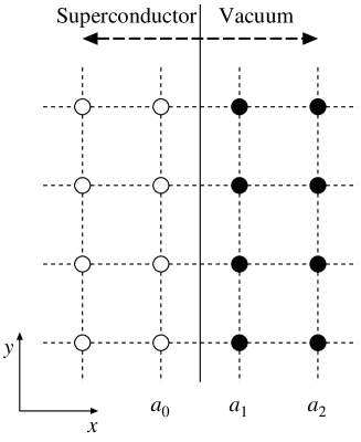
Figure 1: (100) surface of square lattice. White and black circles show the sites without and with potential $V$, respectively.

To calculate SDOS, we construct the Green’s function in semi-infinite system. In the actual numerical calculation, we use the periodic boundary condition along the $x$-direction with a sufficiently large size of mesh. To prepare the (100) surface at $x=a_{0}$, we introduce vacuum layers on the right side of the (100) surface as shown in Fig. 1. Here, it is sufficient to introduce the two vacuum layers since there is no long range hopping or long range pairing over three lattice constant in the present model. On the vacuum layers, we add the following term to the Hamiltonian,

$$\mathcal{H}^{\prime}=V\sum_{x_{i}=a_{1},a_{2}}\sum_{\sigma}n_{i\sigma},$$ (6)

where $n_{i\sigma}=c^{\dagger}_{i\sigma}c_{i\sigma}$ is a number operator at site $i$ with spin $\sigma$, and $V$ is the on-site potential. In the limit $V\rightarrow\infty$, no electron exists on the vacuum layers.

First, we switch on the potential $V$ only at the site $x=a_{1}$. The Green function $\check{G}^{1R}(x_{1},x_{2};k_{y},\omega)$ in this situation satisfies the following equation,

$$\check{G}^{1R}(x_{1},x_{2};k_{y},\omega) = \check{G}^{0R}(x_{1},x_{2};k_{y},\omega)$$ (7)

$$+\check{G}^{0R}(x_{1},a_{1};k_{y},\omega)V\check{\tau}_{3}\check{G}^{1R}(a_{1},x_{2};k_{y},\omega),$$

where $\check{G}^{0R}(x_{1},x_{2};k_{y},\omega)$ is the Fourier component $\check{G}^{0R}({\bm{k}},\omega)$ with respect to $k_{x}$,

$$\check{G}^{0R}(x_{1},x_{2};k_{y},\omega) = \frac{1}{N_{x}}\sum_{k_{x}}\check{G}^{0R}(\bm{k},\omega)e^{ik_{x}(x_{1}-x_{2})}.$$ (8)

Here $N_{x}$ is the number of $x$-meshes, and $\check{\tau}_{3}$ is the Pauli matrix in the particle-hole space.

$$\check{\tau}_{3}=\left(\begin{array}[]{cc}\hat{I}_{2\times 2}&0\\ 0&-\hat{I}_{2\times 2}\end{array}\right).$$ (11)

In the $V\rightarrow\infty$ limit, we have the following solution of Eq. (7),

$$\check{G}^{1R}(x_{1},x_{2};k_{y},\omega) = \check{G}^{0R}(x_{1},x_{2};k_{y},\omega)$$ (12)

$$-\check{G}^{0R}(x_{1},a_{1};k_{y},\omega)\{\check{G}^{0R}(a_{1},a_{1};k_{y},\omega)\}^{-1}$$

$$\hskip 42.67912pt\times\check{G}^{0R}(a_{1},x_{2};k_{y},\omega).$$

Then, we switch on the potential $V$ at the site $x=a_{2}$ as well. For the Green’s function $\check{G}^{2R}(x_{1},x_{2};k_{y},\omega)$ in this case, we have the following equation,

$$\check{G}^{2R}(x_{1},x_{2};k_{y},\omega) = \check{G}^{1R}(x_{1},x_{2};k_{y},\omega)$$ (13)

$$+\check{G}^{1R}(x_{1},a_{2};k_{y},\omega)V\check{\tau}_{3}\check{G}^{1R}(a_{2},x_{2};k_{y},\omega),$$

Therefore, taking the $V\rightarrow\infty$ limit, we obtain the Green’s function in the semi-infinite system,

$$\check{G}^{2R}(x_{1},x_{2};k_{y},\omega) = \check{G}^{1R}(x_{1},x_{2};k_{y},\omega)$$ (14)

$$-\check{G}^{1R}(x_{1},a_{2};k_{y},\omega)\{\check{G}^{1R}(a_{2},a_{2};k_{y},\omega)\}^{-1}$$

$$\hskip 42.67912pt\times\check{G}^{1R}(a_{2},x_{2};k_{y},\omega).$$

From (12) and (14), we can calculate the SDOS $\rho_{\rm s}(\omega)$, which is given by the local density of states at $x=a_{0}$,

$$\rho_{\rm s}(\omega)=-\frac{1}{N_{y}}\sum_{k_{y}}\sum_{\alpha=1,2}{\rm Im}\{G^{2R}_{\alpha\alpha}(a_{0},a_{0};k_{y},\omega)\},$$ (15)

while the DOS in the bulk is given by

$$\rho_{\rm b}(\omega)=-\frac{1}{N_{x}N_{y}}\sum_{k_{x}kS_{y}}\sum_{\alpha=1,2}{\rm Im}\{G^{0R}_{\alpha\alpha}({\bm{k}},\omega)\},$$ (16)

where $N_{x}$ and $N_{y}$ are the number of meshes along the $x$ and the $y$ direction, respectively. In the calculation presented in the following, we choose $N_{x}=N_{y}=2^{13}$. We set $t=\Delta_{0}=1$ for the unit of energy. The number of electrons per unit cell is $0.3$ ($\mu\sim-2.40$). To guarantee the convergence, we use $\eta=0.03t$ for the infinitesimal imaginary parts in Eq. (2).

III Results

In this section, we first focus on the local density of state at the surface, $i.e.$, SDOS $\rho_{\rm s}(\omega)$ for various paring symmetry. Since spin-singlet and spin-triplet components of pair potential mix in general, we introduce a parameter $r_{s}$, which denotes the ratio of singlet component. The parameter $r_{s}$ ($0\geq r_{s}\geq 1$) is defined as $\Delta_{s}=r_{s}\Delta_{0}$ and $\Delta_{t}=(1-r_{s})\Delta_{0}$.

The SDOS for $s+p$-wave case is plotted in Fig. 2. In this case, the bulk DOS $\rho_{\rm b}(\omega)$ always has a $U$-shaped gap structure as shown in solid lines. The magnitude of the gap is given by $\mid\Delta_{s}-\Delta_{t}\mid$. For $\Delta_{s}>\Delta_{t}$, the SDOS $\rho_{\rm s}(\omega)$ also has a $U$-shaped gap structure as shown in the dashes lines in Fig. 2 (a) and (b). On the other hand, for $\Delta_{t}>\Delta_{s}$ with $r_{s}=0.2$ and $r_{s}=0$, the resulting $\rho_{\rm s}(\omega)$ has a residual value at $\omega=0$ as shown in Figs.2(c) and (d), respectively. To show up the SDOS more clearly, we also show the angle resolved surface density of states (ARSDOS) $-\sum_{\alpha=1,2}{\rm Im}\{G^{2R}_{\alpha\alpha}(a_{0},a_{0};k_{y},\omega)\}$. As shown in Fig. 3(a), ARSDOS shows a full gap structure without any inner gap state for singlet dominant case ($\Delta_{s}>\Delta_{t}$). On the other hand, as shown in Fig. 3(b), the ARSDOS for triplet dominant case ($\Delta_{t}>\Delta_{s}$) has two branches of Andreev bound state, which are dubbed as helical edge modes Tanaka ; Sato2009 . The presence of helical edge modes inside the bulk energy gap induces the residual SDOS inside the bulk energy gap.

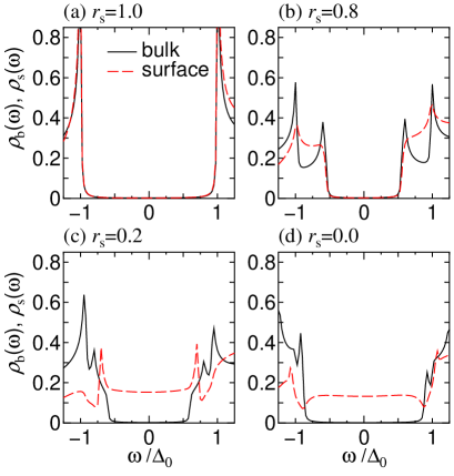
Figure 2: (Color online) Local density of states for $s$+$p$-wave in the bulk (solid lines) and at the surface (dashed lines) for $\lambda=0.5$ and $r_{s}=1.0$, $0.8$, $0.2$, and $0.0$.

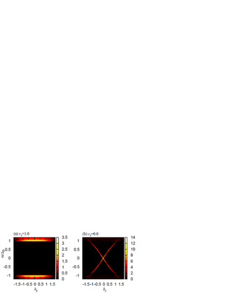
Figure 3: (Color online) Angle resolved local density of state of $s$+$p$-wave pairing is plotted as a function of $k_{y}$ with $\lambda=0.5$. (a)$\Delta_{s}=\Delta_{0}$ and $\Delta_{t}=0$, (b)$\Delta_{t}=\Delta_{0}$ and $\Delta_{s}=0$.

Next we look at SDOS for $d_{x^{2}-y^{2}}+f$-wave case plotted in Fig. 4. In this case, $\rho_{\rm b}(\omega)$ always has a $V$-shaped gap structure as shown in solid lines reflecting the nodal structures of the bulk energy gap. The corresponding $\rho_{\rm s}(\omega)$ (dashed line) also has a similar $V$-shaped gap structure for singlet dominant case ($\Delta_{s}>\Delta_{t}$) with $r_{s}=1$ and $r_{s}=0.8$. As shown in Fig.5(a), there is no inner gap state in ARSDOS, while the bulk energy gap has a strong $k_{y}$-dependence. On the other hand, for triplet dominant case ($\Delta_{t}>\Delta_{s}$) with $r_{s}=0.2$ and $r_{s}=0$, $\rho_{\rm s}(\omega)$ has two additional peaks as shown in dashed lines of Figs.4(c) and (d) as compared to the bulk density of states Mizuno (solid lines). The additional two peaks in the SDOS originates from the helical edge modes generated inside energy gap as shown in Fig. 5(b) Mizuno .

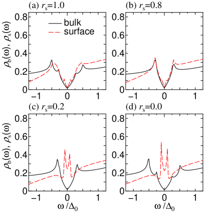
Figure 4: (Color online) Local density of states for $d_{x^{2}-y^{2}}$+$f$-wave in the bulk (solid lines) and at the surface (dashed lines) for $\lambda=0.5$ and $r_{s}=1.0$, $0.8$, $0.2$, and $0.0$.

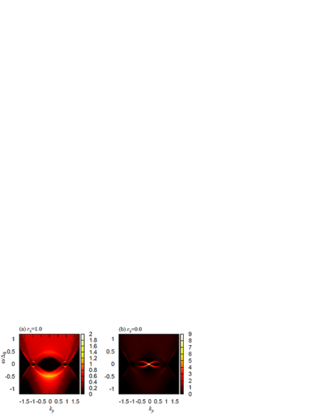
Figure 5: (Color online) Angle resolved local density of state of $d_{x^{2}-y^{2}}$+$f$-wave pairing is plotted as a function of $k_{y}$ with $\lambda=0.5$. (a)$\Delta_{s}=\Delta_{0}$ and $\Delta_{t}=0$, (b)$\Delta_{t}=\Delta_{0}$ and $\Delta_{s}=0$.

The SDOS for $d_{xy}+p$-wave NCS superconductors is plotted in Figs. 6 and 8. In this case, $\rho_{\rm s}(\omega)$ has very different line shapes as compared to former two cases. In particular, for the spin-triplet dominant pairing, we find that the SDOS is very sensitive to the spin-orbit coupling. To show this, we first start with the case without spin-orbit coupling i.e. $\lambda=0$. See Fig. 6. $\rho_{\rm b}(\omega)$ has a $V$-shaped gap structure as shown in solid lines, reflecting on the nodal structure of pair potential. The corresponding $\rho_{\rm s}(\omega)$ (dashed line) has a zero energy peak (ZEP) for singlet dominant case with $r_{s}=1$ and $r_{s}=0.8$. This ZEP comes from the mid gap Andreev bound state with flat dispersion as shown in Fig. 7(a), and it is essentially the same as that appears in the surface state of high-$T_{\rm c}$ cuprate Hu ; TK95 . On the other hand, for triplet dominant case with $r_{s}=0.2$ and $r_{s}=0$, the ZEP disappear, but $\rho_{\rm s}(\omega)$ supports two additional peaks instead, as shown in dashed lines of Figs.6(c) and (d), respectively. The additional two peaks are generated by the anomalous ABS. In the absence of Rashba spin-orbit coupling, the dispersion of the anomalous ABS for $d_{xy}+p$-wave pairing is very similar to the helical edge modes for $d_{x^{2}-y^{2}}+f$-wave pairing, as shown in Fig. 7(b). However, the intensity of ARSDOS near $k_{y}\sim 0$ is very low since the magnitude of the excitation energy of the ABS is close to the bulk energy gap. In the 2D free electron model for NCS superconductor, it is shown that the dispersion of ABS corresponds the bulk energy gap and the intensity of ARSDOS is completely absent for $|k_{y}|<k_{c}$.Mizuno . Thus, in contrast to the helical edge mode in the $d_{x^{2}-y^{2}}+f$-wave pairing case, the values of the SDOS $d_{xy}+p$-wave pairing at $\omega/\Delta=0$ is very close to zero.

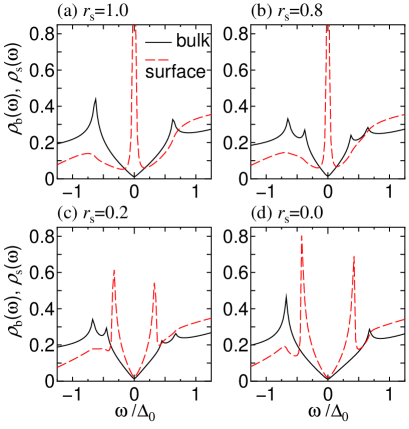
Figure 6: (Color online) Local density of states for $d_{xy}$+$p$-wave in the bulk (solid lines) and at the surface (dashed lines) for $\lambda=0.0$ and $r_{s}=1.0$, $0.8$, $0.2$, and $0.0$.

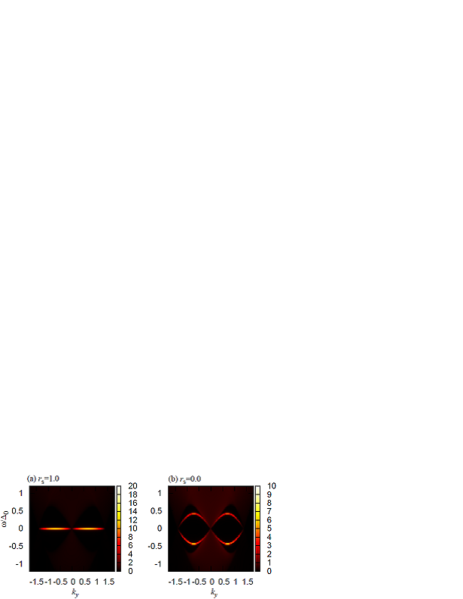
Figure 7: (Color online) Angle resolved local density of state of $d_{xy}$+$p$-wave pairing is plotted as a function of $k_{y}$ with $\lambda=0.0$. (a)$\Delta_{s}=\Delta_{0}$ and $\Delta_{t}=0$, (b)$\Delta_{t}=\Delta_{0}$ and $\Delta_{s}=0$.

Let us now consider the $d_{xy}+p$-wave case with nonzero spin-orbit coupling $\lambda$. As shown in Fig. 8, the bulk DOS $\rho_{\rm b}(\omega)$ shows a $V$-shaped gap structure similar to Fig.6. Then, for singlet dominant case with $r_{s}=1$ and $r_{s}=0.8$, the SDOS $\rho_{s}(\omega)$ (dashed line in Figs. 8(a) and (b), respectively) has a ZEP similar to Figs. 6(a) and (b). On the other hand, for triplet dominant case with $r_{s}=0.2$ and $r_{s}=0$, in addition to two peaks similar to those in Figs. 6(c) and 6(d), ZEP appears as shown in Figs.8(c) and 8(d). It is remarkable that ZEP is generated by spin-orbit coupling $\lambda$ Mizuno .

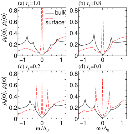
Figure 8: (Color online) Local density of states for $d_{xy}$+$p$-wave in the bulk (solid lines) and at the surface (dashed lines) for $\lambda=0.5$ and $r_{s}=1.0$, $0.8$, $0.2$, and $0.0$.

To show up the new ZEP much more clearly, we plot ARSDOS of $d_{xy}+p$-wave case in Fig. 9 with $\lambda=0.5$. Comparing with the ARSDOS in Fig.7, for triplet dominant case, we find that an additional zero energy state (ZES) appears. In the presence of the spin-orbit coupling, the Fermi surface is split into the large one with the Fermi momenta $k_{2}$ and the small one with $k_{1}$. The ZES exists only for $k_{y}$ between the split Fermi surfaces, namely, for $k_{y}$ with $k_{2}>|k_{y}|>k_{1}$. It can be shown that the Bogoliubov quasiparticle creation operator $\gamma_{\bm{k}}^{\dagger}$ for the ZES satisfies $\gamma_{\bm{k}}^{\dagger}=\gamma_{-{\bm{k}}}$.Mizuno Therefore, the ZES is identified as a Majorana Fermion.

For singlet dominant $d_{xy}+p$-wave NCS superconductors, we obtain the SDOS and ARSDOS depicted in Figs.8(a)-(b) and Fig.9(a), respectively. At first sight, they look very similar to those in Figs.7(a)-(b) and Fig.8. However, for $k_{y}$ with $k_{2}>|k_{y}|>k_{1}$, we again have a single branch of a zero energy state on the edge. As is shown later, because of the existence of the time-reversal invariant Majorana Fermion (TRIMF), the SDOS for the $d_{xy}+p$-wave NCS superconductor shows a peculiar dependence on the Zeeman magnetic field.

Unlike the Majorana Fermions studied before, the present Majorana Fermion is realized with the time reversal invariance. The TRIMF has the following three characteristics. (a) It has a unique flat dispersion. To be consistent with the time-reversal invariance, the single branch of ZES should be symmetric under $k_{y}\rightarrow-k_{y}$. Therefore, by taking into account the particle-hole symmetry as well, the flat dispersion is required. On the other hand, the conventional time-reversal breaking Majorana edge state has a linear dispersion. (b) The spin-orbit coupling is indispensable for the existence of the TRIMF. Without the spin-orbit coupling, the TRIMF vanishes. (c) The TRIMF is topologically stable under small deformation of the Hamiltonian. The topological stability is ensured by a topological number, which will be shown below.

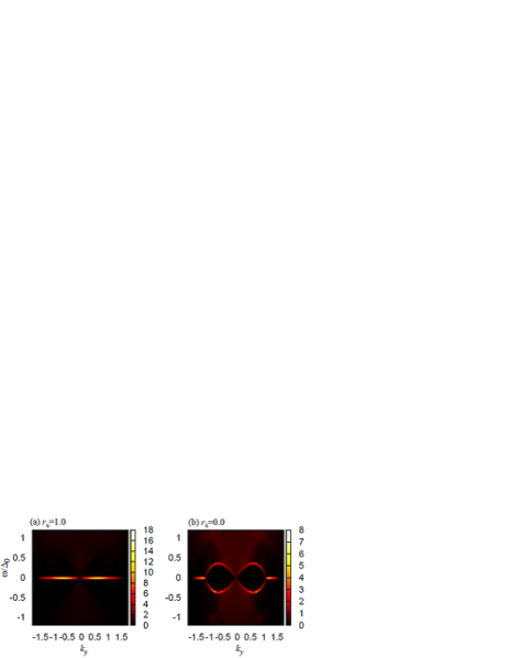
Figure 9: (Color online) Angle resolved local density of state of $d_{xy}$+$p$-wave pairing is plotted as a function of $k_{y}$ with $\lambda=0.5$. (a)$\Delta_{s}=\Delta_{0}$ and $\Delta_{t}=0$, (b)$\Delta_{t}=\Delta_{0}$ and $\Delta_{s}=0$.

To see the topological nature of the TRIMF, we start from the Bogoliubov-de Gennes (BdG) Hamiltonian in the bulk system defined in eq. (5) without Zeeman magnetic field. In the Nambu representation, the BdG Hamiltonian (5) has the particle-hole symmetry,

$$\check{C}\check{\mathcal{H}}({\bm{k}})\check{C}^{\dagger}=-\check{\mathcal{H}}^{*}(-{\bm{k}}),\quad\check{C}=\left(\begin{array}[]{cc}0&\hat{I}_{2\times 2}\\ \hat{I}_{2\times 2}&0\end{array}\right).$$ (19)

In addition, from the time-reversal invariance, the BdG Hamiltonian satisfies

$$\check{\Theta}\check{\mathcal{H}}({\bm{k}})\check{\Theta}^{\dagger}=\check{\mathcal{H}}^{*}(-{\bm{k}}),\quad\check{\Theta}=\left(\begin{array}[]{cc}i\sigma_{y}&0\\ 0&i\sigma_{y}\end{array}\right).$$ (22)

Therefore, we can define the operator $\Gamma$ which anticommutes with the BdG Hamiltonian,

$$\{\check{\mathcal{H}}({\bm{k}}),\check{\Gamma}\}_{+}=0.$$ (23)

Here $\Gamma$ is defined as the product of particle-hole transformation operator $C$ and time reversal operator $\Theta$,

$$\check{\Gamma}=-i\check{C}\check{\Theta}=\left(\begin{array}[]{cc}0&\hat{\sigma}_{y}\\ \hat{\sigma}_{y}&0\end{array}\right).$$ (26)

Now we take the basis which diagonalizes $\check{\Gamma}$

$$\check{U}_{\Gamma}^{\dagger}\check{\Gamma}\check{U}_{\Gamma}=\left(\begin{array}[]{cc}\hat{I}_{2\times 2}&0\\ 0&-\hat{I}_{2\times 2}\end{array}\right)$$ (29)

with the unitary matrix $\check{U}_{\Gamma}$

$$\check{U}_{\Gamma}=\check{U}_{\Gamma}^{\dagger}=\frac{1}{\sqrt{2}}\left(\begin{array}[]{cc}\hat{I}_{2\times 2}&\hat{\sigma}_{y}\\ \hat{\sigma}_{y}&-\hat{I}_{2\times 2}\end{array}\right).$$ (32)

Then, we find that the BdG Hamiltonian $\check{\mathcal{H}}({\bm{k}})$ becomes off-diagonal in this basis,

$$\check{U}_{\Gamma}^{\dagger}\check{\mathcal{H}}({\bm{k}})\check{U}_{\Gamma}=\left(\begin{array}[]{cc}0&\hat{q}({\bm{k}})\\ \hat{q}({\bm{k}})^{\dagger}&0\end{array}\right),$$ (35)

where $\hat{q}({\bm{k}})=\hat{\xi}_{\bm{k}}\hat{\sigma}_{y}-\hat{\Delta}_{\bm{k}}$.

To classify the existence or nonexistence of the ZES with $k_{y}=k_{y}^{0}$, we change $k_{x}$ from $-\pi$ to $\pi$ for a fixed value of $k_{y}=k_{y}^{0}$. The winding number $W$ is defined as a number of revolutions of det$|\hat{q}({\bm{k}})|\equiv m_{1}({\bm{k}})+im_{2}({\bm{k}})$ around the origin of complex plane when $k_{x}$ changes from $-\pi$ to $\pi$,

$$W(k_{y}^{0})=\frac{1}{2\pi}\int_{-\pi}^{\pi}\left.\frac{\partial\theta({\bm{k}})}{\partial k_{x}}\right|_{k_{y}\rightarrow k_{y}^{0}}dk_{x},$$ (36)

with $\theta({\bm{k}})\equiv\arg\det|\hat{q}({\bm{k}})|=\tan^{-1}(m_{2}({\bm{k}})/m_{1}({\bm{k}}))$. The resulting $W(k_{y}^{0})$ must be an integer since the starting point and the end point of integration route are equivalent in the Brillouin zone. Therefore, the value of $W(k_{y}^{0})$ changes discretely with the change of $k_{y}$-value. When the gap of the system closes at certain points on the integration route, $W(k_{y}^{0})$ is ill-defined since det$|\hat{q}({\bm{k}})|$ becomes to zero on such points. Thus, the value of $W(k_{y})$ does not change by the small change of $k_{y}$-value unless the energy gap closes.

Here, we study the winding number for the $d_{xy}+p$-wave NCS superconductors for on the two trajectories for $k_{y}=0.20\pi$ and $0.45\pi$ as shown in Fig. 10. For $k_{y}=0.2\pi$, the trajectory crosses the Fermi surfaces four times. On the other hand, for $k_{y}=0.45\pi$, it crosses two times. As was explained above, the winding number $W(k_{y})$ does not change unless the energy gap closes. For $d_{xy}+p$-wave parings, the energy gap closes at $(\pm k_{1},0)$, $(\pm k_{2},0)$, $(0,\pm k_{1})$ and $(0,\pm k_{2})$. Therefore, $W(k_{y})$ can change only at $k_{y}=\pm k_{1}$, $k_{y}=\pm k_{2}$ or $k_{y}=0$. Thus, it is sufficient to study the representative point in each $k_{y}$ range.

Figure 10: Fermi surfaces of spin-split bands due to the Rashba spin-orbit coupling (solid lines) and cutting lines $k_{y}=0.20\pi$ and $0.45\pi$ (dashed lines).

We first focus on the singlet dominant $d_{xy}+p$-wave NCS superconductor with $\Delta_{s}=\Delta_{0}$ and $\Delta_{t}=0$. For $k_{y}=0.2\pi$, as shown in Fig. 11(a), $m_{1}$ and $m_{2}$ draw a curve which turns anti-clockwise twice around the $(m_{1},m_{2})=(0,0)$ if we change $k_{x}$ from $-\pi$ to $\pi$. At the same time, $\theta({\bm{k}})$ changes twice from $-\pi$ to $\pi$ as shown in Fig. 11(b). Therefore, the resulting winding number $W$ is $W=2$. On the other hand, for $k_{y}=0.45\pi$, $m_{1}$ and $m_{2}$ draw a curve which turns anti-clockwise once around the $(m_{1},m_{2})=(0,0)$ as shown in Fig. 11(c). Moreover, $\theta({\bm{k}})$ changes once from $-\pi$ to $\pi$ as shown in Fig. 11(d). Thus the resulting winding number $W$ equals to $W=1$. This means that these two cases belong to different topological classes. In a similar manner, it is possible to generalize above argument for other $k_{y}$s ($-\pi<k_{y}<\pi$). We summarize the obtained results in Table 1 (a).

	$k_{y}$	$k_{y}>k_{2}$	$k_{2}>k_{y}>k_{1}$	$k_{1}>k_{y}>0$	$0>k_{y}>-k_{1}$	$-k_{1}>k_{y}>-k_{2}$	$-k_{2}>k_{y}$
(a)	$W(k_{y})$	$0$	$1$	$2$	$-2$	$-1$	$0$
(b)	$W(k_{y})$	$0$	$-1$	$0$	$0$	$1$	$0$

Table 1: The winding number $W(k_{y})$ for $d_{xy}+p$-wave with (a) $\Delta_{\rm s}>\Delta_{\rm t}$, (b) $\Delta_{\rm t}<\Delta_{\rm s}$.

Figure 11: Polar plot of $\theta({\bm{k}})$ for $\Delta_{s}=\Delta_{0}$ and $\Delta_{t}=0$ as a function of $k_{x}$ with fixed $k_{y}$, (a) $k_{y}=0.2\pi$ and (c) $k_{y}=0.45\pi$, where white circle corresponds to $k_{x}=\pm\pi$ and arrows show the direction in which the values of $k_{x}$ increase. The corresponding $\theta=\tan^{-1}(m_{2}/m_{1})$ is plotted as a function of $k_{x}$ for (b) $k_{y}=0.2\pi$ and (d) $k_{y}=0.45\pi$.

The same plot of $m_{i}({\bm{k}})$ and $\theta({\bm{k}})$ for the triplet dominant $d_{xy}+p$-wave NCS superconductors with $\Delta_{t}=\Delta_{0}$ and $\Delta_{s}=0$ is shown in Fig. 12. For $k_{y}=0.2\pi$, $m_{1}$ and $m_{2}$ draw a curve as shown in Fig. 12(a). However, it does not turn around the $(m_{1},m_{2})=(0,0)$ with the change of $k_{x}$ from $-\pi$ to $\pi$. At the same time, $\theta({\bm{k}})$ does not change from $-\pi$ to $\pi$ as shown in Fig. 12(b), in contrast to that in Fig. 11(b). This corresponds to the fact that the resulting winding number $W$ equals to $W=0$. On the other hand, for $k_{y}=0.45\pi$, $m_{1}$ and $m_{2}$ draw a curve which turns clockwise once around the $(m_{1},m_{2})=(0,0)$ as shown in Fig. 12(c). Also, $\theta({\bm{k}})$ changes once from $\pi$ to $-\pi$ as shown in Fig. 12(d). Therefore, the corresponding winding number $W$ equals to $W=-1$. In a manner to the singlet dominant case, it is possible to generalize this argument for other $k_{y}$s. ($-\pi<k_{y}<\pi$)The obtained results are summarized in Table 1(b).

Figure 12: Polar plot of $\theta({\bm{k}})$ for $\Delta_{t}=\Delta_{0}$ and $\Delta_{s}=0$ as a function of $k_{x}$ with fixed $k_{y}$, (a) $k_{y}=0.2\pi$ and (c) $k_{y}=0.45\pi$, where white circle corresponds to $k_{x}=\pm\pi$ and arrows show the direction in which the values of $k_{x}$ increase. The corresponding $\theta=\tan^{-1}(m_{2}/m_{1})$ is plotted as a function of $k_{x}$ for (b) $k_{y}=0.2\pi$ and (d) $k_{y}=0.45\pi$.

Comparing the obtained winding number $W(k_{y})$ in Table 1 with the ARSDOS in Fig 9, we notice that zero energy ABS appears only for $k_{y}$ with nonzero $W(k_{y})$. This correspondence implies that the existence and the stability of the zero energy ABS is ensured by the winding number. Indeed, we can say the absolute value of $W$, $i.e.$, $\mid W\mid$ equals to the number of branch of zero energy ABS STYY10 . In other words, the number of TRIMF equals to the absolute value of $W$. Furthermore, the TRIMF found here are topologically stable against a small deformation of the BdG Hamiltonian if the deformation preserves the time-reversal invariance and the translation invariance along the direction parallel to the edge, both of which are necessary to define the winding number. It should be remarked that both for the singlet dominant case and the triplet dominant one, a single TRIMS is generated for $k_{2}>\mid k_{y}\mid>k_{1}$.

As is shown above, the time-reversal invariance is essential to define the winding number $W$ ensuring the topological stability of the TRIMF. Therefore, in general, if we apply a perturbation breaking the time-reversal invariance, the winding number $W$ becomes the meaningless. In other words, a time-reversal breaking perturbation may change the SDOS of the TRIMF substantially.

As a time-reversal breaking perturbation, we consider the Zeeman magnetic field. Let us look at the SDOS in the presence of Zeeman magnetic field ${\bm{H}}$. First, we consider the singlet dominant $d_{xy}+p$-wave NCS superconductor. Without the spin orbit coupling, the Andreev bound state becomes conventional and can be expressed by double TRIMFs. In this case, as we expected, it is found that the zero energy peak of SDOS from the double TRIMF is split into two by any Zeeman magnetic field ${\bm{H}}$ as shown in Fig. 13 Kashiwaya98 . It is also noted that the resulting SDOS is independent of the direction of ${\bm{H}}$ due to the spin-rotational symmetry in the system. Thus, the SDOSs $\rho_{s}(\omega)$ for $\mu_{B}H_{x}=0.1t$ (${\bm{H}}\parallel{\bm{x}}$), $\mu_{B}H_{y}=0.1t$ (${\bm{H}}\parallel{\bm{y}}$) and $\mu_{B}H_{z}=0.1t$ (${\bm{H}}\parallel{\bm{z}}$) are the same.

Figure 13: Local density of states at the surface for $d_{xy}$+$p$-wave with $\Delta_{s}=\Delta_{0}$ and $\Delta_{t}=0$ for $\lambda=0$ and (a) $\mu_{\rm B}{\bm{H}}=0$, (b) $\mu_{\rm B}H_{x}=0.1$ (${\bm{H}}\parallel{\bm{x}}$).

On the other hand, in the presence of the spin-orbit coupling, this property is not satisfied anymore. As shown in Fig.14, $\rho_{s}(\omega)$ has a different values for $\mu_{B}H_{x}=0.1t$ [Fig. 14(b)], $\mu_{B}H_{y}=0.1t$ [Fig. 14(c)] and $\mu_{B}H_{z}=0.1t$ [Fig. 14(d)], respectively. The orientational dependence of SDOS is due to the presence of the spin-orbit coupling since the spin-rotational symmetry is broken. It is noted, three peak structure including zero energy peak appears for $\mu_{\rm B}H_{y}=0.1t$ (${\bm{H}}\parallel{\bm{y}}$). The presence of the remaining ZEP under the Zeeman magnetic field along the edge, which is $H_{y}$ in this case, is relevant to the existence of the single Majorana fermion at $k_{2}>|k_{y}|>k_{1}$. On the other hand, the double TRIMFs at $|k_{y}|<k_{1}$ is split into two for any direction of Zeeman magnetic field. Therefore, the height of ZEP $\rho_{s}(0)$ drastically decrease even if ZEP remains for $\mu_{\rm B}H_{y}=0.1t$ (${\bm{H}}\parallel{\bm{y}}$).

Figure 14: Local density of states at the surface for $d_{xy}+p$-wave with $\Delta_{s}=\Delta_{0}$ and $\Delta_{t}=0$ for $\lambda=0.5$ and (a) $\mu_{\rm B}{\bm{H}}=0$, (b) $\mu_{\rm B}H_{x}=0.1t$ (${\bm{H}}\parallel{\bm{x}}$), (c) $\mu_{\rm B}H_{y}=0.1t$ (${\bm{H}}\parallel{\bm{y}}$), (d) $\mu_{\rm B}H_{z}=0.1t$ (${\bm{H}}\parallel{\bm{z}}$).

Next we consider the triplet dominant $d_{xy}+p$-wave NCS superconductor. For simplicity, we suppose that only the triplet component $\Delta_{p}$ exists. As was shown in Fig.9(b), in the absence of the Zeeman magnetic field, a zero energy ABS exists and it can be described by a single TRIMF. The resulting $\rho_{s}(\omega)$ has a sharp ZEP without ${\bm{H}}$ [Fig. 15(a)]. In a manner similar to the singlet dominant case above, the SDOS $\rho_{s}(\omega)$ under the Zeeman magnetic field has a strong orientational dependence of ${\bm{H}}$ as shown in Figs. 15 (b), (c) and (d). It is noted that ZEP remains when the applied Zeeman field is along $y$-direction. This implies that the single TRIMF in the $d_{xy}+p$-wave NCS superconductor is robust against the Zeeman magnetic field applied in the direction along the edge.

Figure 15: Local density of states at the surface for $d_{xy}$+$p$-wave with $\Delta_{t}=\Delta_{0}$ and $\Delta_{s}=0$ for $\lambda=0.5$ and (a) $\mu_{\rm B}{\bm{H}}=0$, (b) $\mu_{\rm B}H_{x}=0.1t$ (${\bm{H}}\parallel{\bm{x}}$), (c) $\mu_{\rm B}H_{y}=0.1t$ (${\bm{H}}\parallel{\bm{y}}$), (d) $\mu_{\rm B}H_{z}=0.1t$ (${\bm{H}}\parallel{\bm{z}}$).

We would like to emphasis that, as shown from these calculation, the tunneling spectroscopy with the Zeeman magnetic field is available to identify the single TRIMF in the $d_{xy}+p$-wave NCS superconductor. Simultaneous existence of the strong orientational dependence of magnetic field and the robust zero energy peak under a certain direction of the magnetic field is a strong evidence to support single Majorana Fermion in this material.

IV Summary

In the present paper, we have obtained SDOS, edge modes of NCS superconductors by choosing $s+p$, $d_{x^{2}-y^{2}}+f$, and $d_{xy}+p$-wave pair potential based on the lattice model Hamiltonian. For $d_{xy}+p$-wave pairing, special ABS appears as a zero energy state for $k_{2}>\mid k_{y}\mid>k_{1}$ with wavenumber parallel to the interface $k_{y}$, where $k_{1}$ and $k_{2}$ denote the magnitude of the Fermi wavenumber in the presence of spin-orbit coupling. The present ABS is a single Majorana edge mode preserving the time reversal symmetry. We have defined a new type of topological invariant number and clarify the relevance to the number of the time-reversal invariant Majorana edge modes. We have found that the absolute value of the topological number equals to the number of the Majorana edge modes. The single Majorana edge mode is generally induced by the spin orbit coupling. In the presence of the single Majorana edge mode, the SDOS has a strong orientational dependence of the magnetic field. In a certain direction of the applied magnetic field, the single Majorana edge mode is robust and the resulting zero energy peak of SDOS remains. The present future may serve as a guide to detect Majorana Fermion in non-centrosymmetric superconducting superconductors by tunneling spectroscopy.

This work is partly supported by the Sumitomo Foundation (M.S.) and the Grant-in-Aids for Scientific Research No. 22103005 (Y.T. and M.S.), No. 20654030 (Y.T.) and No.22540383 (M.S.).

References

- (1) E. Bauer, G. Hilscher, H. Michor, Ch. Paul, E.W. Scheidt, A. Gribanov, Yu. Seropegin, H. Noël, M. Sigrist, and P. Rogl, Phys. Rev. Lett. 92, 027003 (2004).
- (2) K. Togano, P. Badica, Y. Nakamori, S. Orimo, H. Takeya, and K. Hirata, Phys. Rev. Lett. 93, 247004 (2004); M. Nishiyama, Y. Inada, and G. Q. Zheng, Phys. Rev. B 71, 220505(R) (2005).
- (3) A. D. Hillier, J. Quintanilla, and R. Cywinski, Phys. Rev. Lett. 102, 117007 (2009).
- (4) N. Reyren, S. Thiel S, A. D. Caviglia, L. F. Kourkoutis, G. Hammerl, C. Richter, C. W. Schneider, T. Kopp, A. S. Ruetschi, D. Jaccard, M. Gabay, D.A. Muller, J. M. Triscone, J. Mannhart, Science 317, 1196 (2007).
- (5) L. P. Gor’kov and E. I. Rashba, Phys. Rev. Lett. 87 037004 (2001).
- (6) P. A. Frigeri, D. F. Agterberg , A. Koga and M. Sigrist, Phys. Rev. Lett. 92, 097001 (2004).
- (7) S. Fujimoto, J. Phys. Soc. Jpn. 76, 051008 (2007).
- (8) Y. Yanase and M. Sigrist, J. Phys. Soc. Jpn. 77, 124711 (2008); Y. Tada, N. Kawakami, and S. Fujimoto, New J. Phys.11, 055070 (2009).
- (9) T. Yokoyama, Y. Tanaka and J. Inoue, Phys. Rev. B 72 220504(R) (2005); C. Iniotakis, N. Hayashi, Y. Sawa, T. Yokoyama, U. May, Y. Tanaka, and M. Sigrist, Phys. Rev. B 76, 012501 (2007); M. Eschrig, C. Inotakis, and Y. Tanaka, arXiv:1001.2486.
- (10) A.B. Vorontsov, I. Vekhter, and M. Eschrig, Phys. Rev. Lett. 101, 127003 (2008).
- (11) Y. Tanaka, T. Yokoyama, A. V. Balatsky and N. Nagaosa, Phys. Rev. B 79, 060505(R) (2009).
- (12) M. Sato, Phys. Rev. B 73 214502 (2006); M. Sato and S. Fujimoto, Phys. Rev. B 79, 094504 (2009);
- (13) C.K. Lu and S. Yip, Phys. Rev. B 80, 024504 (2009).
- (14) T. Yokoyama, S. Onari, and Y. Tanaka, Phys. Rev. B 75, 172511 (2007); T. Yokoyama, S. Onari, and Y. Tanaka, J. Phys. Soc. Jpn. 77 064711 (2008).
- (15) K. Yada, S. Onari, Y. Tanaka, and J. Inoue Phys. Rev. B 80 140509 (2009).
- (16) Y. Tanaka, Y. Mizuno, T. Yokoyama, K. Yada and M. Sato, Phys. Rev. Lett. 105, 097002 (2010).
- (17) L. J. Buchholtz and G. Zwicknagl, Phys. Rev. B 23, 5788 (1981); J. Hara and K. Nagai, J. Hara and K. Nagai, Prog. Theor. Phys. 74, 1237 (1986). S. Kashiwaya and Y. Tanaka, Rep. Prog. Phys. 63, 1641 (2000).
- (18) C. R. Hu, Phys. Rev. Lett. 72, 1526 (1994).
- (19) Y. Tanaka and S. Kashiwaya, Phys. Rev. Lett. 74, 3451 (1995).
- (20) M. Covington, M. Aprili, E. Paraoanu, L. H. Greene F. Xu, J. Zhu, and C. A. Mirkin, Phys. Rev. Lett. 79, 277 (1997); L. Alff, H. Takashima, S. Kashiwaya, N. Terada, H. Ihara, Y. Tanaka, M. Koyanagi, and K. Kajimura, Phys. Rev. B 55, R14757 (1997); J. Y. T. Wei, N.-C. Yeh, D. F. Garrigus, and M. Strasik, Phys. Rev. Lett. 81, 2542 (1998); A. Biswas, P. Fournier, M. M. Qazilbash, V. N. Smolyaninova, H. Balci, and R. L. Greene, Phys. Rev. Lett. 88, 207004 (2002); B. Chesca, M. Seifried, T. Dahm, N. Schopohl, D. Koelle, R. Kleiner, and A. Tsukada, Phys. Rev. B 71, 104504 (2005); B. Chesca1, D. Doenitz, T. Dahm, R. P. Huebener, D. Koelle, R. Kleiner, Ariando, H. J. H. Smilde, and H. Hilgenkamp, Phys. Rev. B, 73, 014529 (2006); B. Chesca, H. J. H. Smilde, and H. Hilgenkamp, Phys. Rev. B 77, 184510 (2008).
- (21) Y. Maeno, H. Hashimoto, K. Yoshida, S. Nishizaki, T. Fujita, J. G. Bednorz, and F. Lichtenberg, Nature 372, 532 (1994).
- (22) M. Matsumoto and M. Sigrist, J. Phys. Soc. Jpn. 68, 994 (1999); C. Honerkamp and M. Sigrist, J. Low Temp. Phys. 111, 895 (1998); M. Yamashiro, Y. Tanaka, and S. Kashiwaya, Phys. Rev. B 56, 7847 (1997).
- (23) C. L. Kane and E. J. Mele, Phys. Rev. Lett. 95, 146802 (2005); C. L. Kane and E. J. Mele, Phys. Rev. Lett. 95, 226801 (2005); B. A. Bernevig, and S. C. Zhang, Phys. Rev. Lett. 96, 106802 (2006); B. A. Bernevig, T. L. Hughes, and S. C. Zhang, Science 314 1757 (2006).
- (24) See for e.g., The Quantum Hall effect, edited by R.E. Prange and S.M. Girvin, (Springer-Verlag, 1987), and references therein.
- (25) D. J. Thouless, M. Kohmoto, M. P. Nightingale, and M. den Nijs, Phys. Rev. Lett. 49, 405 (1982).
- (26) L. Fu and C. L. Kane, Phys. Rev. B 74, 195312 (2006); L. Fu and C. L. Kane, Phys. Rev. B 76, 045302 (2007).
- (27) A. P. Schnyder, S. Ryu, A. Furusaki, and A. W. W. Ludwig, Phys. Rev. B 78, 195125 (2008); X.L. Qi, T. L. Hughes, S. Raghu and S.C. Zhang, Phys. Rev. Lett. 102, 187001 (2009); R. Roy, arXiv:cond-mat/0608064. R. Roy, arXiv:0803.2881; M. Sato, Phys. Rev. B 79, 214526 (2009); M. Sato, arXiv:0912.5281.
- (28) L. Fu and C. L. Kane, Phys. Rev. Lett. 100, 096407 (2008); L. Fu and C. L. Kane, Phys. Rev. Lett. 102, 216403 (2009); J. Nilsson, A. R. Akhmerov, and C. W. J. Beenakker, Phys. Rev. Lett. 101, 120403 (2008); A. R. Akhmerov, J. Nilsson, and C. W. J. Beenakker, Phys. Rev. Lett. 102, 216404 (2009); M. Sato, Y. Takahashi, and S. Fujimoto, 103, 020401 (2009); Phys. Rev. Lett. 103, 020401 (2009); Y. Tanaka, T. Yokoyama and N. Nagaosa, Phys. Rev. Lett. 103, 107002 (2009); K. T. Law, P. A. Lee, T. K. Ng, Phys. Rev. Lett. 103, 237001 (2009).
- (29) J. Alicea, Phys. Rev. B 81, 125318 (2010); J. D. Sau, R. M. Lutchyn, S. Tewari, and S. Das Sarma, Phys. Rev. Lett. 104, 040502 (2010); Y. Asano, Y. Tanaka and N. Nagaosa, Phys. Rev. Lett. 105, 056402 (2010); V. Shivamoggi, G. Refael, and J. E. Moore, Phys. Rev. B 82, 041405(R) (2010).
- (30) When the symmetry of the singlet component of pair potential is -wave (-wave), the number of the sign change of the real or imaginary part of triplet one on the Fermi surface is two (six). Thus, we call the mixed pair potential -wave (-wave).
- (31) M.Sato et al., in preparation.
- (32) S. Kashiwaya, Y. Tanaka, N. Yoshida, and M. R. Beasley, Phys. Rev. B 60, 3572 (1999).