Emergence of Cooperation with Self-organized Criticality

Abstract

Cooperation and self-organized criticality are two main keywords in current studies of evolution. We propose a generalized Bak-Sneppen model and provide a natural mechanism which accounts for both phenomena simultaneously. We use the prisoner’s dilemma games to mimic the interactions among the members in the population. Each member is identified by its cooperation probability, and its fitness is given by the payoffs from neighbors. The least fit member with the minimum payoff is replaced by a new member with a random cooperation probability. When the neighbors of the least fit one are also replaced with a non-zero probability, a strong cooperation emerges. The Bak-Sneppen process builds a self-organized structure so that the cooperation can emerge even in the parameter region where a uniform or random population decreases the number of cooperators. The emergence of cooperation is due to the same dynamical correlation that leads to self-organized criticality in replacement activities.

I Introduction

A fundamental question in the theory of evolution has been how cooperation can emerge between selfish members Nowak06B ; Nowak:sci.06 ; Milinski87 ; Segbroeck09 ; Gomez07 ; Parcheco06 ; Santos05 . Another question is why evolution takes place in terms of intermittent bursts of activities, which are the characteristics of dynamical systems in a ‘critical’ state Gould77 ; Raup86 . Here, we propose a generalized Bak-Sneppen (BS) model Bak93 , which may solve the above two puzzles simultaneously. We take an approach of evolutionary game theory and use the prisoner’s dilemma (PD) games to mimic the interactions among members. Each member is identified by its stochastic strategy, specified by its (history independent) cooperation probability (CP). Here, a ‘member’ can represent an individual in a species, an agent in an economical system or a species in an ecological system. The fitness of a member is given by the payoffs of the games with its neighbors. We then apply BS dynamics and replace the least fit member and its neighbors by new members with random CPs. The neighbors of the non-cooperator are likely to vanish due to its low payoff, but the non-cooperator itself can also be removed through the BS mechanism. As the non-cooperators disappear, the overall CP increases, and a new comer (with a random CP) will have a lower CP than the increased average. Therefore, the new comer tends to cause its neighbor to be the least fit, and the replacement activity likely occurs at or near the new comer’s site. This invokes the spatio-temporal correlation between the least fit sites and can explain why replacements are episodic as well as how cooperation emerges.

Evolutionary game theory has been one of the most powerful tools in studying the dynamics of evolution Nowak06B . However, a simple straightforward application of game theory cannot explain the strong cooperation between “selfish” replicators observed in nature and society. For the evolution to construct a new, upper level of organization, cooperation amongst the majority of the population is needed. However, the game theoretical description of interactions between members usually leads to defections as evolutionarily stable strategies. Natural selection, which has been a fundamental principle of evolution, prefers the species that beat off the others and oppose cooperation.

There have been numerous studies looking for natural mechanisms for the evolution of cooperation among competitive members Hamilton64 ; Milinski87 ; nowak:nat.98 ; West02 . Recently, Nowak presented a state-of-art review on the evolution of cooperation and discussed five known mechanisms: kin selection, direct reciprocity, indirect reciprocity, network reciprocity, and group selection Nowak:sci.06 ; Grafen:JEB.07 . Extensive studies provide the exact conditions for the emergence of cooperation for each of the five mechanisms. However, such conditions do not seem to be general enough to explain the cooperative phenomena observed everywhere. For example, for network reciprocity, the benefit-to-cost ratio of a cooperative behavior should be larger than the average degree Nowak:sci.06 , but this seems to be a rather strong assumption because the degrees are quite large in most cases in real population structures. Also, there have been a great deal of studies on self-organized criticality in game theory Scheinkman:AMR94 ; Sole:JTB95 ; Killingback:JTB98 ; Arenas:EDC02 ; Ebel:PRE02 , but their dynamics leading to the critical states are not directly connected to the emergence of cooperation. Here, we consider an evolutionary game on networks and show that cooperation can emerge when the benefit to cost ratio is larger than just 1 if we use the BS process. When cooperators interact with defectors, they tend to disappear, giving rise to an assortment of cooperators Fletcher:PRSB.09 . Furthermore, this behavior emerges in the long run even with a small “chain-death” rate, $\omega$, where the number of neighbors that get replaced is less than one. For a uniform or random arrangement of cooperators and defectors, more cooperators than defectors disappear for small $\omega$, but in the long run, the BS process builds a self-organized structure so that the number of cooperators in the population increases.

II model

An influential model aimed to mimic the interactions between competitive members in a population is the PD game. It is one of the matrix games between two players who have two possible decisions, cooperation ($C$) or defection ($D$). We consider a case in which the payoffs are calculated by the cost $c$ and the benefit $b$ of a cooperative behavior. If one player defects while the other cooperates, the defector receives benefit $b$ without any cost whereas the cooperator pay cost $c$ and its payoff becomes $-c$. For mutual cooperation, both get benefit $b$, but pay cost $c$, and their payoffs become $b-c$ while the payoffs for mutual defection are 0. When we add $c$ to all elements so that payoff can be directly interpreted as (non-negative) fitness, the payoff matrix becomes

$$\begin{array}[]{cc}&\ \ \begin{array}[]{cc}C&D\end{array}\\ \begin{array}[]{c}C\\ D\end{array}&\left(\begin{array}[]{cc}b&0\\ b+1&1\\ \end{array}\right),\\ \end{array}$$

where we set $c=1$ without loss of generality. With conventional competition processes, the matrix game shown above does not, in general, predict the evolution of cooperation. The birth-death process always predicts an evolution of defection. Cooperation can emerge for death-birth or imitation processes in a structured population, but only with a (unrealistic) large value of the benefit-to-cost ratio $b$ for real populations Nowak:sci.06 .

Here, we consider the PD game interaction, but introduce the BS mechanism Bak93 as the competition process, and assume that the least fit member and its neighbors are prone to disappear. Each member is characterized by its strategy that determines when to choose the ‘decisions’ $C$ or $D$. We consider the history-independent stochastic strategies, and the phenotype of a member, say the $i$th member, is represented by its CP $c_{i}$. The history independent pure (deterministic) strategies, the “always $C$” and the “always $D$”, correspond to the limits of $c_{i}=1$ and $c_{i}=0$, respectively. The fitness of a member is given by the sum of payoffs from its neighbors, and the member dies out if its total payoff is the minimum. The died-out site is occupied by a new member with a new CP, which is drawn randomly from 0 to 1. Neighbors of the least fit site may also be harmed in the process of establishing the steady interaction with the new comer. Hence, we replace the neighbors of the least fit site by new members with the “chain-death” probability $\omega>0$.

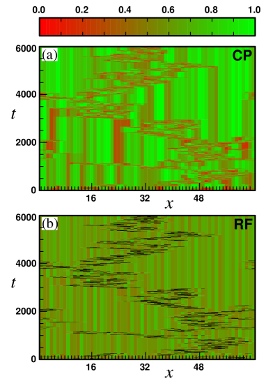
Figure 1: Real space configurations of (a) the CP $c_{i}$ and (b) the RF $\tilde{f}_{i}$ for $t\in[0,6000]$ with $\omega=1$ and $N=64$. They are represented by colors, red for 0 and green for 1, as indicated by the top panel. The black dots in (b) represent the least fit sites.

III Methods and Results

We study the strategy evolution of a simple structured population from the initial state of random strategies. Initially, members in the population have cooperation probabilities that are drawn randomly from the uniform distribution of the interval [0 1]. They play PD games with their nearest neighbors. We assume that each member plays sufficiently many games prior to the reproduction process and use the payoff expectation value as its fitness. The least fit member with the minimum payoff expectation is replaced by a new member with a new random CP. In addition to the least fit member, the neighbors of the least fit member are also replaced by new members with the probability $\omega$. Then, we recalculate the payoff expectations, and replacements occur at the new least fit member and its neighbors. We continue these processes until the system reaches a steady state and calculate the statistical properties of the population, such as the mean cooperation probability, fitness distribution, avalanche size (defined later) distribution and etc.

For simplicity, we present our model and results in a one-dimensional (1D) structure, but our main results hold in other population structures. Initially ($t=0$), we assign a random CP, $c_{i}(0)$, to the site $i$ for $i=1,\ldots,N$. Then, we calculate the payoff expectation, $f_{i}(0)$, at time $t=0$,

$$f_{i}(0) = b\,\left[{c_{i-1}(0)+c_{i+1}(0)}\right]+2\left[{1-c_{i}(0)}\right],$$ (1)

of site $i$ with a periodic boundary condition and find the minimum payoff site, $m_{0}$. Except this minimum site, $m_{0}$ and its neighbors, $m_{0}\pm 1$, the CPs are not changed at $t=1$, so we set $c_{i}(1)=c_{i}(0)$ unless $i=m_{0}$ or $m_{0}\pm 1$. The CP at the $m_{0}$ site, $c_{m_{0}}(1)$, is given by a new random number between 0 and 1. For its neighbor sites, $c_{m_{0}\pm 1}(1)$ is given by a new independent random number with the probability $\omega$, but remains as $c_{m_{0}\pm 1}(0)$ with the probability $1-\omega$. Now, we recalculate the payoff $f_{i}$ of Eq. (1) with $c_{k}(1)$ instead of $c_{k}(0)$. We find the new minimum payoff site, $m_{1}$, of $t=1$ and apply the same replacement dynamics to get $t=2$ configurations and so on.

Figure 1 shows typical real space configurations of CP, $c_{i}$, and the reduced fitness (RF), $\tilde{f}_{i}=f_{i}/(2b+2)\in[0\ 1]$. We show the configurations for initial 6000 time steps of a $N=64$ system with $b=1.5$ and $\omega=1$. Both the CP and the RF are represented by colors, 0 by red and 1 by green. The least fit sites (black sites in (b)) and their two neighbors are where the replacement activity occurs. Comparison between the configurations in (a) and their equivalents in (b) reveals that the least fit sites are located where their neighbors are less cooperative [relatively red in (a)]. The disappearance of the “red” neighbors beside the least fit site by the BS-mechanism shifts the overall system to green (more cooperative) with time.

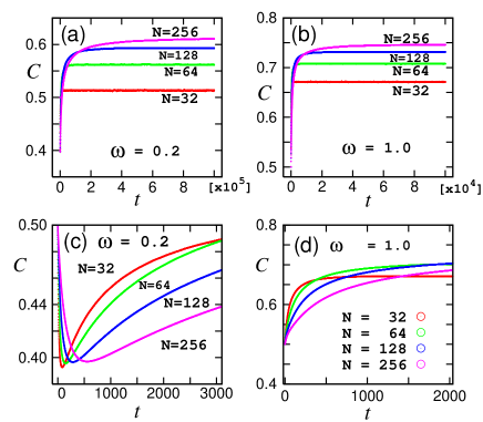
Figure 2: Time dependence of MCP, $C$, for (a,c) $\omega=0.2$ and (b,d) $\omega=1.0$ for systems with $N=32$, 64, 128, and 256. In (a) and (b), the overall behaviors of MCP are shown while the initial transient characteristics are shown in (c) and (d). For $\omega=0.2$, MCP decreases first and then increases while it monotonically increases for $\omega=1$.

For a quantitative analysis, we measure the mean CP (MCP), $C(t)=\langle{\frac{1}{N}\sum_{i}c_{i}(t)}\rangle$, of the populations and show the results in Fig. 2. Here, $\langle{\cdot}\rangle$ represents the ensemble average over many different realizations of random initial configurations. Note that the MCP also represents the overall fitness $F(t)=\langle{\frac{1}{N}\sum_{i}f_{i}(t)}\rangle$ of the population because it is linearly related to MCP:

$$F(t) = \frac{1}{N}\langle{\sum_{i}b\,\left[{c_{i-1}(t)+c_{i+1}(t)}\right]+2\left[{1-c_{i}(t)}\right]}\rangle$$ (2)

$$= 2+2(b-1)C(t).$$

In Fig. 2, the MCPs for four different system sizes, $N=32$, 64, 126, and 256, are shown for two different values of $\omega$, $0.2$, and 1. We use $b=1.5$ for all figures in this paper, and all data are obtained from numerical simulations. Because we have assigned a random CP initially, the MCP starts from 0.5 at $t=0$. For $\omega=0.2$, the MCP decreases at the beginning and then increases to the steady values while it monotonically increases from the beginning for $\omega=1$, as shown in Figs. 2(c) and (d). Note that we have two different elements in MCP changes. Replacement of the least fit member (which is likely to have a high CP) tends to cause the MCP to decrease while the replacement of its neighbors (which probably have low CPs) likely results in an increased MCP. The competition between these two elements governs the early dynamics of the MCP. It can decrease initially when $\omega<\omega_{c}\approx\frac{1}{k}=1/2$, where $k$ is the number of neighbors. For a sufficiently large system, there would be a site, $m$, whose CP, $c_{m}$, is arbitrarily close to one while those of its neighbors, $c_{m\pm 1}$, are almost zero. Hence, the expectation of MCP changes, $\Delta MCP$ would be $\frac{1}{N}\left[{\left({\frac{1}{2}-1}\right)+k\omega\left({\frac{1}{2}-0}\right)}\right]$ and becomes negative for $\omega<\frac{1}{k}$ at the beginning. However, as time proceeds, the CP values develop spatio-temporal correlations, and they govern the long-time dynamics. Initially, the isolated high-CP cooperators are likely to be the least fit member, and they are removed as time proceeds. Then, surviving cooperators remain in the groups, and, thus, have high fitness. Now, low-CP defectors can be the least fit member, especially when they are next to a very low-CP member. The replacement of these low-CP member by new members with random CPs causes the MCP to increase. Therefore, at a later time, the MCP easily becomes larger than the initial 0.5 even for $\omega<\omega_{c}$. Now, a new comer with a random CP will have a lower CP than the increased average of MCP. This in turn causes the least fit site to be likely located next to the new comer’s site, resulting in avalanches of replacement activities.

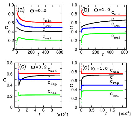
Figure 3: Evolution of the CPs of the least fit members, $C_{min}$, their neighbors, $C_{nei}$, and members that are replaced, $C_{rep}$, are shown together with MCP, $C$, for (a,c) $\omega=0.2$, and (b,d) $\omega=1.0$. In (a) and (b), the initial transient behaviors are shown while overall behaviors are shown in (c) and (d). The system size $N=128$ is used for all cases.

IV Analysis of the initial dynamics

We start from the population with random strategies. Hence, there is no correlation between the CPs initially, and we may understand the initial dynamics through the mean-field calculation. We first define the mean CP of the replacement sites (before the replacement),

$$C_{rep} = \frac{1}{1+2\omega}(C_{min}+2\omega C_{nei}),$$ (3)

where mean-field dynamics can be easily analyzed. Here, $C_{min}$ is the average of the CPs for the least fit members, and $C_{nei}$ is that for the neighbors of the least fit members. On average, CPs of $1+2\omega$ sites are updated each time. Since the average of the newly assigned random cooperation rate is 0.5, $C_{rep}$ satisfies,

$$\frac{dC_{rep}}{dt} = \frac{1}{1+2\omega}\left[{(0.5-C_{min})+2\omega(0.5-C_{nei})}\right]$$ (4)

$$= 0.5-C_{rep}.$$

We measure $C_{rep}$ and present them in Fig. 3, together with the CPs of the least fit members, $C_{min}$, that of the replaced members, $C_{rep}$, and the MCP, $C$, for $\omega=0.2$ and $\omega=1.0$. The $C_{rep}$ curves are, indeed, well described by Eq. (4). If we represent the numerical solutions of Eq. (4) in the figure, they cannot be distinguished from the $C_{rep}$ curves from the simulations because they are almost identical. From Fig. 3, we also see that $C_{rep}$ enters its steady value in a relatively short period of time compared to $C$ and rapidly converges to its steady-state value of 0.5. For $\omega=0.2$, the initial $C_{rep}$ is more than half and hence decreases to the steady value of 0.5 while it increases from the value below 0.5 for $\omega=1.0$. For a sufficiently large system, the initial value of $C_{min}$ would be 1 while $C_{nei}$ is 0. Hence, the initial value of $C_{rep}$ would be $\frac{1}{1+2\omega}$, which is more than 0.5 for $\omega<1/2$. In this transient time of $C_{rep}$, the dynamics of MCP, $C$, would be mainly determined by the dynamics of $C_{rep}$. Therefore, $C$ initially decreases for $\omega<1/2$ as does $C_{rep}$. However, after $C_{rep}$ reaches a steady value, the correlation of the replacement sites mainly governs the dynamics, and $C$ begins to increase. Let $m$ be the least fit member at time $t-1$; then, at time $t$, $c_{m}$ is always updated, and $c_{j=m\pm 1}$ are updated with probability $\omega$. After replacement, if the sum of the CPs at these three sites, $s_{rep}(t)=c_{m}(t)+\sum_{j=m\pm 1}c_{j}(t)$ (at the time $t$), is small, at least one of $m-1$, $m$ or $m+1$ sites, is likely to have small fitness. Therefore, they will be easily replaced in a relatively short time. In other words, a new born member with small $s_{rep}(t)$ has a short lifetime and contributes less to the $C$ than those with large $s_{rep}(t)$. This mechanism makes $C$ increase up to (almost) $C_{min}$, and hence, the system becomes cooperative overall. Thus, according to our model, the emergence of cooperation is intrinsically related to the dynamics leading to self-organized criticality (SOC).

V Self organized criticality

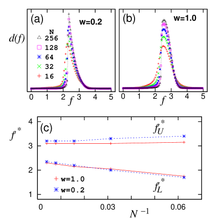
Figure 4: Fitness distribution $d(f)$ in the steady states for five different system sizes of $N=16$, 32, 64, 128 and 256 with (a) $\omega=0.2$ and (b) $\omega=1.0$. The system size dependence of the effective lower and upper thresholds $f_{L}^{*}$ and $f_{U}^{*}$ (defined in the text) are shown in (c). Legends of (a) are also applied to (b).

We now show that our model, in fact, drives the population into a SOC state as in the original BS model. We measure the distributions of avalanche sizes and distances between successive least fit sites in the steady states and show that they follow power-law distributions.

Following Bak and Sneppen Bak93 , we would like to define the size of an avalanche as the number of subsequent replacements at the least fit sites below the lower threshold $f_{L}$ in its fitness value. The fitness distributions $d(f)$ share some characteristics of the BS model Bak93 although their overall shapes are quite different. A crucial similarity is that the fitness distribution $d(f)$ in the steady state becomes zero for fitness $f$ smaller than a lower threshold $f_{L}$ as the system size goes to infinity.

The fitness distributions in the steady states for five different system sizes are shown in Figs. 4(a) and (b) for $\omega=0.2$ and $\omega=1.0$. As the system sizes increase, the peak positions of the fitness distribution move to the right to high values, and the peak widths become narrow. To estimate the threshold values $f_{L}$ and $f_{U}$, we define the effective lower [upper] threshold $f_{L}^{*}(N)$ [$f_{U}^{*}(N)$] as the $f$ value below [above] which the integrated distribution is 5 percent. We plot them against $1/N$ in Fig. 4(c) for two different chain-death rates, $\omega=0.2$ and $\omega=1.0$. There are no noticeable differences in the thermodynamic values for the two $\omega$ values. Using linear fitting, we get rough estimates of the threshold values, $f_{L}=2.4\pm 0.05$ and $f_{U}=3.1\pm 0.1$, for both $\omega$ values.

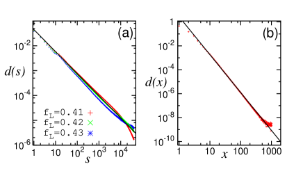
Figure 5: (a) Distributions $d(s)$ of avalanche sizes $s$. Distributions with three different values of $f_{L}$, $f_{L}=2.41$, $f_{L}=2.42$, and $f_{L}=2.43$ are measured in systems of $N=256$ in their steady states. Data with $f_{L}=2.42$ show a most persistent straight line in the log-log scale fit, indicating the lower threshold $f_{L}=2.42$ for the $N=256$ system with $\omega=1$. The black line is the least-squares fit of the data for $f_{L}=2.42$ and is given in a form of $d(s)\sim s^{-\tau}$ with $\tau=0.89\pm 0.05$. (b) A distribution $d(x)$ of the distances between successive minimum fitness sites in the steady states for the system of $N=2048$ with $\omega=1$. The black line is the least squares fit of the data in the form of $d(x)=ax^{-\alpha}$ with $\alpha=3.17\pm 0.03$.

For the avalanche size distribution $d(s)$, we need a more precise value of $f_{L}$. We measure $d(s)$ with several different values of $f_{L}$ around the estimated value. If the system is really in a SOC state, we expect the avalanche size distribution $d(s)$ to show a power-law distribution, for the exact value of $f_{L}$ for the given system. Figure 5(a) shows the distribution of avalanche sizes in a system of size $N=256$. We plot $d(s)$ against $s$ on a log-log scale with three different values of $f_{L}$ around the value estimated from Fig. 4(c) to pinpoint the threshold $f_{L}$. For $\omega=1.0$ shown in Fig. 5(a), the avalanche size distribution is well fit by a power-law with $f_{L}=2.42$. It remains as a line in the log-log plot up to an avalanche size about 20000, indicating power-law distributions $d(s)\sim s^{-\tau}$. The exponent obtained from a least-square fit of the form $d(s)=Ay^{-\tau}$ is $\alpha=0.89\pm 0.05$. This value is consistent with the known exponent of the 1D BS model Bak93 . The power law indicates that the evolution occurs in a dynamical criticality Bak93 ; Bak96B . We measure the avalanche distributions for other $\omega$ and $b$ and found the critical exponent $\tau$ to be independent of the benefit-to-cost ratio $b$ or the chain-death probability $\omega$.

We also measured the distance distribution between successive least fit sites. Denoting the distance between successive minimum fitness sites by $y$, we plot $d(y)$ in Fig. 5(b). The distance distribution is measured in the steady states for the system of $N=2048$ with $\omega=1$. When the distribution $d(y)$ is plotted against $y$ on a log-log scale, it also becomes a line, indicating power-law distributions $d(y)\sim y^{-\alpha}$ with the slop $\alpha=3.17\pm 0.03$. This exponent is also consistent with the known exponent of the 1D BS model Bak93 . It is notable that our model belongs to the same universality class as the BS model in spite of the complexity in computing the fitness of members and the non-trivial dynamics of the population-fitness changes.

VI Concluding Remarks

We have considered the BS mechanism as a reproduction process with fitness given by a PD game payoff on a network structure. Our observation may have more natural implication in economical systems because the BS process with chain bankruptcy is a more feasible scenario. It might be worthwhile analyzing weekly or monthly bankruptcy data and see if they follow a power-law distribution as our study suggests.

We have simulated our model with other values of the benefit-to-cost ratio $b$ and see that cooperation emerges in a wide range of chain-death rates $\omega$, as long as $b$ is larger than 1. In contrast to a common belief, cooperation can emerge even with parameters that a population with random strategies decreases cooperation. This is possible because the BS mechanism builds dynamical correlations that suppress the long-term survival of non-cooperators even in the region where mean-field calculation predicts a decrease in cooperators. The same dynamical correlation leads to SOC in replacement activities with the same exponents as the original BS model. The strategy space presented here is rather small. Mixed but only history independent strategies are considered on a very simple population structure, a 1D lattice. However, we speculate that our main results, the emergence of cooperation and SOC, are robust under variations in the population structure or the strategy space extension. In fact, the preliminary results with the extended strategy space show that the emergence of cooperation appears more easily and rapidly when the reactive strategies are included.

VII Acknowledgements

This work was supported by the National Research Foundation of Korea Grant funded by the Korean Government(MEST) (NRF-2010-0022474). H.-C. J. would like to thank KIAS for the support during the visit.

References

- (1) M. A. Nowak, Evolutionary Dynamics (The Belknap Press of Harvard University Press, Cambridge, 2006).
- (2) M. A. Nowak, Science 314, 1560 (2006).
- (3) M. Milinski, Nature 325, 433 (1987).
- (4) S. VanSegbroeck, F. C. Santos, T. Lenaerts, and J. M. Pacheco, Phys. Rev. Lett. 102, 058105 (2009).
- (5) J. Gomez-Gardenes, M. Campillo, L. M. Floria, and Y. Moreno, Phys. Rev. Lett. 98, 108103 (2007).
- (6) J. M. Pacheco, A. Traulsen, and M. A. Nowak, Phys. Rev. Lett. 97, 258103 (2006).
- (7) F. C. Santos and J. M. Pacheco, Phys. Rev. Lett. 95, 098104 (2005).
- (8) S. J. Gould and N. Eldredge, Paleobiology 3, 115 (1977).
- (9) D. M. Raup, Science 231, 1528 (1986).
- (10) P. Bak and K. Sneppen, Phys. Rev. Lett. 71, 4083 (1993).
- (11) W. D. Hamilton, J. Theor. Biol. 7, 1 (1964).
- (12) M. A. Nowak and K. Sigmund, Nature 393, 573 (1998).
- (13) S. A. West, I. Pen, and A. S. Griffin, Science 296, 72 (2002).
- (14) A. Grafen, J. Evol. Bio. 20, 2278 (2007).
- (15) J. A. Scheinkman and M. Woodford, The American Economic Review 84, 417 (1994).
- (16) R. V. Sole and S. C. Manrubia, J. Theor. Biol. 173, 31 (1995).
- (17) T. Killingback and M. Doebeli, J. Theor. Biol. 191, 335 (1998).
- (18) A. Arenas, A. Diat-Guilera, C. J. Perez, and F. Vega-Redondo, J. Econ. Dyna. & Cont. 26, 2115 (2002).
- (19) H. Ebel and S. Bornholdt, Phys. Rev. E 66, 056118 (2002).
- (20) J. A. Fletcher and M. Doebeli, Proc. R. Soc. B 276, 13 (2009).
- (21) P. Bak, How Nature Works (Springer-Verlag, New York, 1996).