$\bm{B\to D^{*}l\nu}$ at zero recoil: an update

Abstract:

We present an update of our calculation of the form factor for $\bar{B}\to D^{*}l\bar{\nu}$ at zero recoil, with higher statistics and finer lattices. As before, we use the Fermilab action for $b$ and $c$ quarks, the asqtad staggered action for light valence quarks, and the MILC ensembles for gluons and light quarks (Lüscher-Weisz married to 2+1 rooted staggered sea quarks). In this update, we have reduced the total uncertainty on $\mathcal{F}(1)$ from 2.6% to 1.7%.

At Lattice2010 we presented a still-blinded result, but this writeup includes the unblinded result from the September 2010 CKM workshop.

1 Introduction

The $Wbc$ vertex is proportional to the coupling $V_{\mathrm{cb}}$, which is an element of the Cabibbo [1] Kobayashi-Maskawa [2] (CKM) matrix. Along with the quark masses, it represents the observable part of the quarks’ coupling to the Higgs sector and is, thus, a fundamental part of particle physics. The CKM matrix has four free parameters, and it is convenient to choose one of them to be (essentially) $|V_{\mathrm{cb}}|$. Consequently, $|V_{\mathrm{cb}}|$ appears throughout flavor physics [3].

$|V_{\mathrm{cb}}|$ is determined from semileptonic decays $\bar{B}\to X_{c}l\bar{\nu}$, where $X_{c}$ denotes a charmed final state. In exclusive decays, $X_{c}$ is a $D$ or $D^{*}$ meson, and the decay amplitudes can be written

$$\langle D(v_{D})|\mathcal{V}^{\mu}|\bar{B}(v_{B})\rangle \!=\! \sqrt{M_{B}M_{D}}\,\left[(v_{B}+v_{D})^{\mu}h_{+}(w)+(v_{B}-v_{D})^{\mu}h_{-}(w)\right],$$ (1)

$$\langle D^{*}(v_{D},\alpha)|\mathcal{V}^{\mu}|\bar{B}(v_{B})\rangle \!=\! \sqrt{M_{B}M_{D^{*}}}\,\varepsilon^{\mu\nu}_{\hphantom{\mu\nu}\rho\sigma}\bar{\epsilon}^{(\alpha)}_{\nu}v^{\rho}_{B}v^{\sigma}_{D^{*}}h_{V}(w),$$ (2)

$$\langle D^{*}(v_{D},\alpha)|\mathcal{A}^{\mu}|\bar{B}(v_{B})\rangle \!=\! i\sqrt{M_{B}M_{D^{*}}}\,\bar{\epsilon}_{\nu}^{(\alpha)}\!\left\{g^{\nu\mu}(1+w)h_{A_{1}}(w)-v^{\nu}_{B}[v^{\mu}_{B}h_{A_{2}}(w)+v^{\mu}_{D^{*}}h_{A_{3}}(w)]\right\},\hskip 20.00003pt$$ (3)

where $\epsilon^{(\alpha)}$ is the $D^{*}$ polarization vector, $v_{B}$ and $v_{D^{(*)}}$ denote the mesons’ 4-velocities, and $w=v_{B}\cdot v_{D^{(*)}}$ is related to the invariant mass of the $l\nu$ pair, $q^{2}=M_{B}^{2}+M_{D^{(*)}}^{2}-2wM_{B}M_{D^{(*)}}$. The form factors $h_{\pm}$, $h_{V}$, and $h_{A_{i}}$ ($i=1,2,3$) enjoy simple heavy-quark limits and are linear combinations of the form factors $f_{\pm}$, $V$, and ${A_{i}}$ used in other semileptonic decays.

The differential decay distributions are

$$\frac{d\Gamma(\bar{B}\to Dl\bar{\nu})}{dw} = \frac{G^{2}_{F}}{48\pi^{3}}m^{3}_{D}(M_{B}+M_{D})^{2}(w^{2}-1)^{3/2}|V_{cb}|^{2}|\mathcal{G}(w)|^{2},$$ (4)

$$\frac{d\Gamma(\bar{B}\to D^{*}l\bar{\nu})}{dw} = \frac{G^{2}_{F}}{4\pi^{3}}m^{3}_{D^{*}}(M_{B}-M_{D^{*}})^{2}(w^{2}-1)^{1/2}|V_{cb}|^{2}\chi(w)|\mathcal{F}(w)|^{2},$$ (5)

neglecting the charged lepton and neutrino masses. The physical combinations of form factors are

$$\mathcal{G}(w) = h_{+}(w)-\frac{M_{B}-M_{D}}{M_{B}+M_{D}}h_{-}(w)=\frac{2\sqrt{M_{B}M_{D}}}{M_{B}+M_{D}}f_{+}(q^{2}),$$ (6)

$$\mathcal{F}(w) = h_{A_{1}}(w)\frac{1+w}{2}\sqrt{\frac{H^{2}_{0}(w)+H^{2}_{+}(w)+H^{2}_{-}(w)}{3\chi(w)}}\to h_{A_{1}}(1),$$ (7)

where the zero-recoil ($w\to 1$) limit of $\mathcal{F}$ is shown. The function $\chi(w)$ is chosen so that the square root in Eq. (7) collapses to 1 if $h_{V}=h_{A_{3}}=h_{A_{1}}$ and $h_{A_{2}}=0$, as in the heavy-quark limit without radiative corrections. Expressions for $H_{\pm}(w)$, $H_{0}(w)$, and $\chi(w)$ can be found in Ref. [3].

The messy formula for $\mathcal{F}(w)$ indicates the advantage of the zero-recoil limit for $\bar{B}\to D^{*}l\bar{\nu}$: one must compute only $h_{A_{1}}(1)$, not four functions. In addition, the heavy-quark flavor symmetry is larger when $v_{D^{*}}=v_{B}$, and Luke’s theorem applies. For determining $|V_{\mathrm{cb}}|$, the key aspect of Luke’s theorem is that it helps control systematic errors. In particular, in lattice gauge theories that respect heavy-quark symmetry, one can compute $h_{A_{1}}(1)$ with heavy-quark discretization errors that are formally $\bar{\Lambda}/m_{Q}$ times smaller than those of $h_{A_{1}}(w)$, $w\neq 1$, or those of $\mathcal{G}(w)$ even at $w=1$.

Here we focus on $\bar{B}\to D^{*}l\bar{\nu}$ at zero recoil, describing our calculations of $\mathcal{F}(1)=h_{A_{1}}(1)$. Starting in 2001, experimental determinations of $|V_{\mathrm{cb}}|$ used a quenched calculation [4]

$$\mathcal{F}(1)=0.913^{+0.024}_{-0.017}\pm 0.016^{+0.003}_{-0.014}{}^{+0.000}_{-0.016}{}^{+0.006}_{-0.014},$$ (8)

where the errors stem, respectively, from statistics, matching lattice gauge theory to QCD, lattice-spacing dependence, chiral extrapolation, and the quenched approximation. A notable feature of Eq. (8) is that an estimate of the error associated with quenching has been made. Nevertheless, it is necessary to incorporate the light- and strange-quark sea. The first calculation with 2+1 flavors of sea quarks obtained [5]

$$\mathcal{F}(1)=0.921\pm 0.013\pm 0.008\pm 0.008\pm 0.014\pm 0.003\pm 0.006\pm 0.004,$$ (9)

where, now, the errors stem from statistics, the $g_{D^{*}D\pi}$ coupling, chiral extrapolation, discretization errors, matching, and two tuning errors. (The catch-phrases for the errors do not have exactly the same meaning in Refs. [4, 5]; for example, the $g_{D^{*}D\pi}$ error in Eq. (8) is incorporated into the chiral-extrapolation error.) This paper presents an update of the 2+1-flavor calculation, with mostly the same ingredients, but with higher statistics and without the second of the tuning errors.

The new data set is shown in Table 1, based as before on the MILC ensembles [6] with the Lüscher-Weisz gauge action [7], with the $g^{2}N_{c}$ [8] but not $g^{2}N_{f}$ corrections [9], and the asqtad-improved [10] rooted staggered determinant for the sea quarks.

Table 1: Parameters of the MILC ensembles used for heavy-quark physics. Here $C$ denotes the number of configurations in each ensemble; $(m^{\prime}_{l},m^{\prime}_{s})$ the asqtad sea-quark masses; $m_{q}$ the asqtad valence masses; $\kappa$ and $c_{\mathrm{SW}}$ the hopping parameter and clover coupling of the heavy quark. Standard nicknames for the lattice spacings are noted ($a\approx 0.045$ fm is “ultrafine”). Data are being generated on all ensembles for all $m_{q}$ inside the $\{\cdots\}$, but the present analysis uses at most two, namely $m_{q}=m^{\prime}_{l}$ and $m_{q}=0.4m^{\prime}_{s}$.

$a$ (fm)	Lattice		$C$	$(am^{\prime}_{l}$,	$am^{\prime}_{s})$	$m_{q}$		$\kappa_{\mathrm{b}}$	$\kappa_{\mathrm{c}}$	$c_{\mathrm{SW}}$
$\approx 0.15$	16${}^{3}\times$	48	596	(0.0290,	0.0484)	{0.0484,	0.0453,
medium	16${}^{3}\times$	48	640	(0.0194,	0.0484)	0.0421,	0.0290,
coarse	16${}^{3}\times$	48	631	(0.0097,	0.0484)	0.0194,	0.0097,	0.0781	0.1218	1.570
	20${}^{3}\times$	48	603	(0.0048,	0.0484)	0.0068,	0.0048}
$\approx 0.12$	20${}^{3}\times$	64	2052	(0.02,	0.05)	{0.05,	0.03,	0.0918	0.1259	1.525
coarse	20${}^{3}\times$	64	2259	(0.01,	0.05)	0.0415,	0.0349,	0.0901	0.1254	1.531
	20${}^{3}\times$	64	2110	(0.007,	0.05)	0.02,	0.01,	0.0901	0.1254	1.530
	24${}^{3}\times$	64	2099	(0.005,	0.05)	0.007,	0.005}	0.0901	0.1254	1.530
$\approx 0.09$	28${}^{3}\times$	96	1996	(0.0124,	0.031)	{0.031,	0.0261,	0.0982	0.1277	1.473
fine	28${}^{3}\times$	96	1946	(0.0062,	0.031)	0.0124,		0.0979	0.1276	1.476
	32${}^{3}\times$	96	983	(0.00465,	0.031)	0.0093,	0.0062,	0.0977	0.1275	1.476
	40${}^{3}\times$	96	1015	(0.0031,	0.031)	0.0047,	0.0031}	0.0976	0.1275	1.478
$\approx 0.06$	48${}^{3}\times$	144	668	(0.0072,	0.018)	{0.0188,	0.0160,	0.1052	0.1296	1.4276
superfine	48${}^{3}\times$	144	668	(0.0036,	0.018)	0.0072,		0.1052	0.1296	1.4287
	56${}^{3}\times$	144	800	(0.0025,	0.018)	0.0054,	0.0036,
	64${}^{3}\times$	144	826	(0.0018,	0.018)	0.0025,	0.0018}
$\approx 0.045$	64${}^{3}\times$	192	860	(0.0028,	0.014)	{0.014, 0.0056, 0.0028}

For the valence quarks, we use the asqtad action for the light quark and the Fermilab interpretation [11] of the clover action [12] for the heavy quark. In this report, we use all ensembles in Table 1 with entries for the heavy-quark couplings ($\kappa_{\mathrm{b}}$, $\kappa_{\mathrm{c}}$, and $c_{\mathrm{SW}}$), except the fine $32^{3}\times 96$ lattice. These data are being generated as part of a broad program of heavy-quark physics, including other semileptonic decays [13] and neutral-meson mixing and decay constants [14].

Improvements to $\mathcal{F}(1)$ are timely [3], because the values of $|V_{\mathrm{cb}}|$ that follow from inclusive decays are in a $2.2\sigma$ tension with those that follow from Eq. (9) and also from $\bar{B}\to Dl\bar{\nu}$ and $\mathcal{G}(1)$ [15]. The result described below is but one aspect of a resolution of the discrepancy. Others include a re-examination of the extrapolation to zero recoil, unquenched lattice-QCD calculations at $w\neq 1$, lattice-QCD calculations by other groups [16], and the incorporation of higher-order corrections to the inclusive decay expressions.

In Sec. 2, we discuss details of the data and of the data analysis. Because the value of $\mathcal{F}(1)$ has been studied so much in the past, any new analysis could be influenced in subtle human ways. To circumvent any such bias, we hide the numerical value of $\mathcal{F}(1)$ via an offset in the matching factor $\rho_{A^{\mathrm{cb}}}$, explained in Sec. 3. We present our preliminary results, with all sources of uncertainty estimated, in Sec. 4. We include the unblinded value here, which was revealed after Lattice 2010 but before these proceedings.

2 Data analysis

As in Ref. [5], we aim for the direct double-ratio

$$\mathcal{R}_{A_{1}}=\frac{\langle D^{*}|\bar{c}\gamma_{j}\gamma_{5}b|\bar{B}\rangle\langle\bar{B}|\bar{b}\gamma_{j}\gamma_{5}c|D^{*}\rangle}{\langle D^{*}|\bar{c}\gamma_{4}c|D^{*}\rangle\langle\bar{B}|\bar{b}\gamma_{4}b|\bar{B}\rangle}=\left|h_{A_{1}}(1)\right|^{2},$$ (10)

where the expressions here are all in (continuum) QCD. To this end, we use lattice gauge theory to compute the three-point correlation functions

$$C^{B\to D^{*}}(t_{i},t_{s},t_{f}) = \sum_{\bm{x},\bm{y}}\langle 0|{\cal O}_{D^{*}}(\bm{x},t_{f})\overline{\Psi}_{\mathrm{c}}\gamma_{j}\gamma_{5}\Psi_{\mathrm{b}}(\bm{y},t_{s}){\cal O}^{\dagger}_{B}(\bm{0},t_{i})|0\rangle,$$ (11)

$$C^{B\to B}(t_{i},t_{s},t_{f}) = \sum_{\bm{x},\bm{y}}\langle 0|{\cal O}_{B}(\bm{x},t_{f})\overline{\Psi}_{\mathrm{b}}\gamma_{4}\Psi_{\mathrm{b}}(\bm{y},t_{s}){\cal O}^{\dagger}_{B}(\bm{0},t_{i})|0\rangle,$$ (12)

$$C^{D^{*}\to D^{*}}(t_{i},t_{s},t_{f}) = \sum_{\bm{x},\bm{y}}\langle 0|{\cal O}_{D^{*}}(\bm{x},t_{f})\overline{\Psi}_{\mathrm{c}}\gamma_{4}\Psi_{\mathrm{c}}(\bm{y},t_{s}){\cal O}^{\dagger}_{D^{*}}(\bm{0},t_{i})|0\rangle,$$ (13)

where $\mathcal{O}_{B}$ and $\mathcal{O}_{D^{*}}$ are interpolating operators coupling to the $B$ and $D^{*}$ mesons, and $\overline{\Psi}_{\mathrm{c}}\gamma_{\mu}\Psi_{\mathrm{b}}$ and $\overline{\Psi}_{\mathrm{c}}\gamma_{\mu}\gamma_{5}\Psi_{\mathrm{b}}$ are improved currents [11, 4, 17, 5]. Then the lattice ratio

$$R_{A_{1}}(t)=\frac{C^{B\to D^{*}}(0,t,T)C^{D^{*}\to B}(0,t,T)}{C^{D^{*}\to D^{*}}(0,t,T)C^{B\to B}(0,t,T)}$$ (14)

should reach a plateau for a range of $t$, $T\gg t\gg 1$. The relationship between the plateau value of $R_{A_{1}}^{1/2}$ and $h_{A_{1}}(1)$ is discussed in Sec. 3.

With staggered fermions, $\mathcal{O}_{B}$ and $\mathcal{O}_{D^{*}}$ couple to both parities, and three-point correlation functions have four distinct contributions:

$$C^{X\to Y}(0,t,T) = \sum_{k=0}\sum_{\ell=0}(-1)^{kt}(-1)^{\ell(T-t)}A_{\ell k}e^{-M^{(k)}_{X}t}e^{-M^{(\ell)}_{Y}(T-t)}$$ (16)

$$= A^{X\to Y}_{00}e^{-M_{X}t-M_{Y}(T-t)}+(-1)^{T-t}A^{X\to Y}_{01}e^{-M_{X}t-M_{Y}^{\prime}(T-t)}+$$

$$(-1)^{t}A^{X\to Y}_{10}e^{-M_{X}^{\prime}t-M_{Y}(T-t)}+(-1)^{T}A^{X\to Y}_{11}e^{-M_{X}^{\prime}t-M_{Y}^{\prime}(T-t)}+\cdots$$

with time-dependent factors of $-1$ associated with the states of undesired parity. To reduce the magnitude of the oscillating components, we form the combination [5]

$$\bar{R}_{A_{1}}(0,t,T)=\textstyle\frac{1}{2}R_{A_{1}}(0,t,T)+\textstyle\frac{1}{4}R_{A_{1}}(0,t,T+1)+\textstyle\frac{1}{4}R_{A_{1}}(0,t+1,T+1),$$ (17)

which should tend more quickly to a plateau. The key here is to have $t_{f}=T$ and $T+1$.

The correlation functions and their ratios are analyzed for two light valence quark masses per ensemble, namely, $m_{q}=m^{\prime}_{l}$ and $m_{q}=0.4m^{\prime}_{s}$ (or the single $m_{q}$ when $m^{\prime}_{l}=0.4m^{\prime}_{s}$). The choice of a fixed $m_{q}$, here $0.4m^{\prime}_{s}$, for all $m^{\prime}_{l}$ matches, by design, our plans for the ultrafine lattice ($a\approx 0.045$ fm), to anchor future analyses even closer to the continuum limit. Typical plateaus are shown in Fig. 1 for a coarse, a fine, and a superfine ensemble.

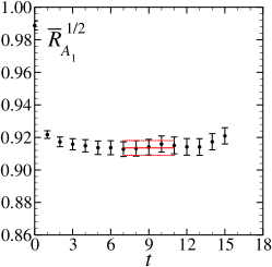
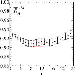
Figure 1: Ratio combination $\bar{R}_{A_{1}}^{1/2}(0,t,T)$ vs. $t$ with $m_{q}=m^{\prime}_{l}=0.2m^{\prime}_{s}$. From left to right: the coarse ensemble with $T=12$ and $(am^{\prime}_{l},am^{\prime}_{s})=(0.01,0.05)$; the fine ensemble with $T=17$ and $(am^{\prime}_{l},am^{\prime}_{s})=(0.0062,0.031)$; the superfine ensemble with $T=24$ and $(am^{\prime}_{l},am^{\prime}_{s})=(0.0036,0.018)$.

As one can see, the plateau in $\bar{R}_{A_{1}}$ emerges readily, and the statistical errors are 1% or smaller.

3 Matching, blinding, and discretization effects

The ratio combination $\bar{R}_{A_{1}}$ tends to a ratio of matrix elements like $\mathcal{R}_{A_{1}}$ in Eq. (10) but with lattice currents. Each current must be multipled by a matching factor $Z_{A}$ or $Z_{V}$, defined nonperturbatively in Ref. [17]. The lattice ratio $R_{A_{1}}$ must, therefore, be multiplied by a matching ratio

$$\rho_{A^{\mathrm{cb}}}^{2}=Z_{A^{\mathrm{cb}}}^{2}/Z_{V^{\mathrm{cc}}}Z_{V^{\mathrm{bb}}}.$$ (18)

A subset of the collaboration has computed $\rho_{A^{\mathrm{cb}}}$ in the one-loop approximation. The result is very close to unity, but the deviation is, or could be, comparable to $h_{A_{1}}(1)-1$. Our numerical analysis replaces $\rho_{A^{\mathrm{cb}}}$ with $F_{\mathrm{blind}}\rho_{A^{\mathrm{cb}}}$, where the blinding factor $F_{\mathrm{blind}}$ is again close to unity, but known only to those engaged in the one-loop calculation. In this way, choices of fitting ranges, etc., cannot be influenced by a human desire to (dis)agree with results for $\mathcal{F}(1)$ already in the literature.

The HQET-Symanzik formalism used to define the $Z_{J}$ can also be used to control and suppress cutoff dependence [18, 17]. In the general case, several operators—both corrections to the current and insertions of the effective Lagrangian—generate cutoff effects. For details, see, e.g., the discussion of Eq. (2.40) in Ref. [17]. For zero recoil, $v_{D^{*}}=v_{B}$, and the heavy-quark flavor symmetry enlarges from $\mathrm{U}(1)\times\mathrm{U}(1)$ to $\mathrm{SU}(2)$. The leading discretization errors drop out, and the remainder can be found by applying the formulas of Ref. [18] to $\bar{R}_{A_{1}}^{1/2}$ and $h_{A_{1}}(1)$. One finds

$$\rho_{A^{\mathrm{cb}}}\bar{R}_{A_{1}}^{1/2}=h_{A_{1}}(1)+\mathrm{O}(\alpha_{s}a\bar{\Lambda}^{2}/m_{\mathrm{c}})+\mathrm{O}(\alpha_{s}a^{2}\bar{\Lambda}^{2})+\mathrm{O}(\alpha_{s}^{2}),$$ (19)

where the last error acknowledges the one-loop calculation of $\rho_{A^{\mathrm{cb}}}$. A study of the asymptotic behavior of Fermilab actions provides a reasonable guide to the dependence on $m_{Q}a$ of the corrections. We see in our data little dependence on the lattice spacing, in accord with Eq. (19).

4 Preliminary result

Figure 2 provides a glimpse into our systematic error analysis, which closely follows Ref. [5].

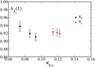
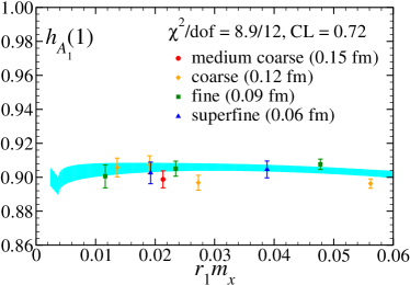
Figure 2: Left: dependence of $h_{A_{1}}(1)$ on the heavy-quark hopping parameters (with data of Ref. [5]). Right: chiral extrapolation showing only points with $m_{q}=m_{l}$ and a fit to all data.

We use our previous study of heavy-quark-mass dependence to fine-tune a posteriori the hopping parameters and to assess the tuning errors. We fit the light-quark mass dependence to one-loop chiral perturbation theory, suitably modified for staggered quarks [19]. The cusp is a necessary, physical effect that appears because the $D\pi$ threshold sinks below the $D^{*}$ mass.

With the blinding factor in place, we find

$$F_{\mathrm{blind}}\mathcal{F}(1)=0.8949\pm 0.0051\pm 0.0088\pm 0.0072\pm 0.0093\pm 0.0030\pm 0.0050,$$ (20)

where the errors again stem from statistics, the $g_{D^{*}D\pi}$ coupling, chiral extrapolation, discretization errors, matching, and tuning $\kappa_{\mathrm{c}}$ and $\kappa_{\mathrm{b}}$. To show how the errors have been reduced, it helps to scale this result to the old central value ($F_{F}$ is the needed ad hoc factor):

$$\mathcal{F}(1) = 0.921(13)(8)(8)(14)(3)(6)(4)~{}\textrm{\cite[cite]{[\@@bibref{}{Bernard:2008dn}{}{}]}},$$ (21)

$$F_{F}\mathcal{F}(1) = 0.921(05)(9)(7)(10)(3)(5)~{}~{}~{}~{}~{}~{}\,\textrm{[this work]}.$$ (22)

The higher statistics and wider scope of this dataset has reduced the statistical error with $C^{-1/2}$. The quoted heavy-quark discretization error is smaller, because with the superfine data we can move beyond pure power counting and combine the (lack of) trend in the data with the detailed theory of cutoff effects [18]. After Lattice 2010, we continued to examine the heavy-quark discretization and $\kappa$-tunings errors, reducing them somewhat, and the chiral-extrapolation error, increasing it somewhat. For the 2010 Workshop on the CKM Unitarity Triangle, we removed the blinding factor, finding [20]:

$$\mathcal{F}(1)=0.9077(51)(88)(84)(90)(30)(33).$$ (23)

This result reduces the tension with $|V_{\mathrm{cb}}|$ from inclusive decays to $1.6\sigma$.

Computations for this work were carried out in part on facilities of the USQCD Collaboration, which are funded by the Office of Science of the U.S. Department of Energy. This work was supported in part by the U.S. Department of Energy under Grants No. DE-FC02-06ER41446 (C.D., L.L., M.B.O), No. DE-FG02-91ER40661 (S.G.), No. DE-FG02-91ER40677 (C.M.B., A.X.K., E.D.F.), No. DE-FG02-91ER40628 (C.B, E.D.F.), No. DE-FG02-04ER-41298 (D.T.); the National Science Foundation under Grants No. PHY-0555243, No. PHY-0757333, No. PHY-0703296 (C.D., L.L., M.B.O), No. PHY-0757035 (R.S.), No. PHY-0704171 (J.E.H.) and No. PHY-0555235 (E.D.F.). C.M.B. was supported in part by a Fermilab Fellowship in Theoretical Physics and by the Visiting Scholars Program of Universities Research Association, Inc. R.S.V. acknowledges support from BNL via the Goldhaber Distinguished Fellowship.

References

• [1] N. Cabibbo, Phys. Rev. Lett.  10 (1963) 531.
• [2] M. Kobayashi and T. Maskawa, Prog. Theor. Phys.  49 (1973) 652.
• [3] M. Antonelli et al., Phys. Rept.  494 (2010) 197 [arXiv:0907.5386 [hep-ph]].
• [4] S. Hashimoto, A.S. Kronfeld, P.B. Mackenzie, S.M. Ryan, and J.N. Simone, Phys. Rev.  D 66 (2002) 014503 [arXiv:hep-ph/0110253].
• [5] C. Bernard et al. [Fermilab Lattice and MILC Collaborations], Phys. Rev.  D 79 (2009) 014506 [arXiv:0808.2519 [hep-lat]].
• [6] A. Bazavov et al., Rev. Mod. Phys. 82 (2010) 1349 [arXiv:0903.3598 [hep-lat]].
• [7] M. Lüscher and P. Weisz, Commun. Math. Phys.  97 (1985) 59 [Erratum ibid.  98 (1985) 433].
• [8] M. Lüscher and P. Weisz, Phys. Lett.  B 158 (1985) 250.
• [9] Z. Hao, G.M. von Hippel, R.R. Horgan, Q.J. Mason, and H.D. Trottier, Phys. Rev.  D 76 (2007) 034507 [arXiv:0705.4660 [hep-lat]].
• [10] G.P. Lepage, Phys. Rev. D 59 (1999) 074502 [hep-lat/9809157].
• [11] A.X. El-Khadra, A.S. Kronfeld, and P.B. Mackenzie, Phys. Rev.  D 55 (1997) 3933 [arXiv:hep-lat/9604004].
• [12] B. Sheikholeslami and R. Wohlert, Nucl. Phys.  B 259 (1985) 572.
• [13] J.A. Bailey et al. [Fermilab Lattice and MILC Collaborations], PoS(Lattice 2010)306.
• [14] C.M. Bouchard et al. [Fermilab Lattice and MILC Collaborations], PoS(Lattice 2010)299.
• [15] M. Okamoto et al. [Fermilab Lattice and MILC Collaborations], Nucl. Phys. Proc. Suppl.  140 (2005) 461 [arXiv:hep-lat/0409116].
• [16] G.M. de Divitiis, E. Molinaro, R. Petronzio, and N. Tantalo, Phys. Lett.  B 655 (2007) 45 [arXiv: 0707.0582 [hep-lat]]; G.M. de Divitiis, R. Petronzio, and N. Tantalo, Nucl. Phys.  B 807 (2009) 373 [arXiv:0807.2944 [hep-lat]].
• [17] J. Harada, S. Hashimoto, A.S. Kronfeld, and T. Onogi, Phys. Rev.  D 65 (2002) 094514 [arXiv:hep-lat/0112045].
• [18] A.S. Kronfeld, Phys. Rev.  D 62 (2000) 014505 [arXiv:hep-lat/0002008].
• [19] J. Laiho and R. S. Van de Water, Phys. Rev.  D 73 (2006) 054501 [arXiv:hep-lat/0512007].
• [20] P.B. Mackenzie, talk at Workshop on the CKM Unitarity Triangle, Warwick, UK (September 2010).