Glassiness in Uniformly Frustrated Systems

Abstract

We review several models of glassy systems where the randomness is self generated, i.e. already an infinitesimal amount of disorder is sufficient to cause a transition to a non-ergodic, glassy state. We discuss the application of the replica formalism developed for the spin glass systems to study the glass transition in uniformly frustrated many-body systems. Here a localization in configuration space emerges leading to an entropy crisis of the system. Using a combination of density functional theory and Landau theory of the glassy state, we first analyze the mean field glass transition within the saddle point approximation. We go beyond the saddle point approximation by considering the energy fluctuations around the saddle point and evaluate the barrier height distribution.

I Introduction

The glass transition and slow glassy dynamics are phenomena most widely studied in the context of supercooled liquids and polymer melts Angel96 ; ang88 . Important progress has been made in understanding the complexity of these phenomena by combining dynamical approaches with the concept of an underlying energy landscape, as is discussed in detail in other chapters of this volume. For example, on the level of the mean field theory of glasses, it has been demonstrated that the dynamical, ideal mode coupling theory mc and energy landscape based replica mean field theories describe the same underlying physics, yet from rather different perspectives KT87 ; KW87 . Novel replica approaches have been developed to characterize the emergence of a metastable amorphous solid Mon95 ; Franz95 ; MePa98.1 ; MePa98.2 . In addition, droplet arguments have been proposed to include important physics beyond the pure mean field description and led to the formulation of the random first order transition theory of glasses KTW89 . The latter is particularly important if one wants to make specific predictions for experiments that require one to go beyond the mean field limit XW00 ; XW01 ; Lubchenko01 ; Lubchenko04a ; Biroli04 . This random first order transition theory of glasses with an underlying entropy crisis Kauzmann48 offers a general and quantitative description of structural glasses. In addition, it defines a universality class for complex many body systems that is of importance for a much larger class of materials.

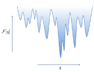
Figure 1: Free energy of a system with entropy crisis as a function of the generalized coordinate $q$. For a specific case of a structural glass $q$ plays a role of density of the local atomic configurations. Glassy behavior is characterized by the emergence of large number of metastable states separated by high energy barriers.

Glassy dynamics usually occurs when a system is supercooled below a first order transition to an ordered state. In supercooled liquids this ordered state is the crystalline solid. If one applies the same ideas to systems with charge or spin collective degrees of freedom in a correlated material, the ordered state corresponds to an electron crystal or an ordered magnetic state. The equilibrium state is therefore ordered. Supercooling the liquid state is possible once the nucleation barriers are high. Thus, in what follows we ignore this ordered state and consider time scales that are short compared to the nucleation time $t_{\mathrm{nucl}}$. One can now ask the question whether and for how long one can still consider the supercooled liquid in local equilibrium. Here, by local equilibrium we mean that the system is ergodic and all configurations are being explored with a probability given by the Boltzmann distribution (only excluding the sharp peak that corresponds to the ordered state). One expects that this supercooled state will fall out of equilibrium over very long time scales, i.e. behave nonergodically, once the barriers between distinct configurations of comparable energy become very large, Fig. 1. If this happens, the system will explore only a subset of the available phase space and will eventually freeze. Suppose there are $\mathcal{N}_{ms}$ of such metastable configurations, that are separated by high barriers, Fig. 2. A calorimetric measurement will then yield an entropy that is reduced by

$$S_{c}\simeq k_{B}\log\mathcal{N}_{ms}$$ (1)

compared to the ergodic situation, where $S_{c}$ is referred to as the configurational entropy. If $\mathcal{N}_{ms}$ is exponentially large in the system size, $S_{c}$ becomes extensive and the dynamically frozen state strictly speaking does not obey the third law of thermodynamics. For liquids it appears that $S_{c}$ on infinite time scales would extrapolate to zero at a temperature $T_{K}>0$. Extrapolating further to $T<T_{K}$ would give $S_{c}$ less then zero. This is the entropy crisis of Kauzmann [16]. Such a crisis is avoided by an ideal glass transition in the models highlighted here.

A crucial question to explore is under what circumstances the configurational entropy is a well defined and meaningful concept. Metastable states become sharp conceptually only within a mean field theory description, where barriers can be infinitely high and a system might get trapped in a local minimum of phase space forever. Within mean field theory, the number of states that are separated by high barriers proliferates at the mode coupling temperature $T_{A}$. The sudden onset of $S_{c}\left(T\right)$ at $T=T_{A}$ should not be misunderstood to mean that new configurations emerge at that temperature. These configurations were present already in the liquid state above $T_{A}$. What happens at $T_{A}$ is that the barriers grow and that the system’s dynamics becomes localized in configuration space. It is this localization in configuration space that is the key element of the random first order theory (not the ultimate glass transition). Within mean field theory the system freezes right at $T_{A}$, while activated events, that are a key element of the theory, allow for a slowed down dynamics even below $T_{A}$, reflecting the fact that those barriers are large but finite.

One might criticize this approach since going beyond mean field theory does not allow for a sharp thermodynamic definition of $S_{c}$. However, there are well known examples that demonstrate the opposite: understanding overheated or supercooled phases close to a first order transition also starts from the mean field concept of a local minimum in the energy landscape. Once supplemented with an appropriate droplet theory of the metastable state it yields a description of the nucleation dynamics at first order transitionsLanger67 . The logic used in the random first order theory of glasses is very similar. One first develops a mean field theory and then supplements it by an appropriate droplet calculation that clearly goes beyond strict mean field theory.

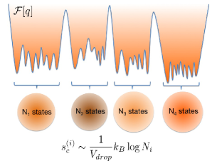
Figure 2: Emergence of an exponentially large number of metastable configurations and the possibility for a system to realize these configurations gives rise to the configurational entropy. The latter serves as the driving force for the structural transitions in the glassy phase.

There are numerous indications that the underlying principles that govern glassy behavior in supercooled liquids apply to other many body systems as well. Generally, glassy systems are characterized by slow relaxations and a broad spectrum of excitations, a behavior found in a number of strongly correlated hard condensed matter physics systems.  A particularly interesting situation occurs when interactions, that change very differently with distance, compete with one another. In such uniformly frustrated systems an intermediate length scale can emerge that leads to new spatial structures and inhomogeneities. A classical example is a ferromagnet where finite range exchange interactions compete with the long range dipole-dipole interactions and leads to the formation of magnetic domains. Similar behavior is in fact abundant in a number of correlated electron systems. Examples are stripe formation in doped Mott insulators stripe ; stripe2 ; mang01 ; Millis96 ; Dagotto ; nmr01 ; nmr02 ; nmr03 ; nmr3b ; nmr04 ; msr01 ; msr02 , defect formation in two-dimensional electron systems Popovich07 ; Spivak2006 ; 2DSpivak2010 , bubbles of electronic states of high Landau levels in quantum Hall systems QHE ; QHE2 , magnetic domains in magnetic multilayer compounds magmtlyr , and mesoscopic structures formed in self-assembly systems selfassbl . These systems typically exhibit a multi-time-scale dynamics similar to the relaxation found in glasses. This observation suggests that glassy behavior and large relaxation times are caused by the competition of interactions with different characteristic length scales Popovic2002 ; Popovic2 ; Vlad2002 ; Denis2002 ; Ohta86 ; Kivelson ; Nussinov ; Schmalian ; SWW00 ; WSW03 ; WSW04 , and not primarily due to the presence of strong disorder in the system. As we will see, this does not mean that disorder is irrelevant for uniformly frustrated systems. In fact, the opposite is true. We find that even the smallest amounts of disorder and imperfections drive such system into a non-ergodic regime that otherwise emerges only in the presence of very strong disorder. In the language of a renormalization group flow this means that the strength of disorder, $g$, flows to larger and larger values  and reaches a strong-disorder fixed point $g^{\ast}$, even if the physical, bare disorder strength is very small. Glassiness arises spontaneously even for infinitesimal extrinsic disorder, leading to self-generated randomness, Fig. 3. In uniformly frustrated systems self generated randomness and the emergence of an entropy crisis were first discussed in Ref. SWW00 . For a beautiful example of self generated randomness in the context of coupled Josephson junction arrays, see Ref. CIS98 .

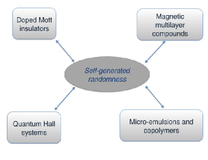
Figure 3: Phenomenon of self-generated randomness appears in a variety of physical systems ranging from strongly correlated two-dimensional electrons to polymer melts and mesoscopic self-assembly structures.

While frustration through competing interactions is easiest to analyze, the notion that uniform geometric frustration is at the heart of the structural glass transition was already discussed and analyzed in Refs.Sadoc ; Nelson ; Sethna with the underlying view that one can capture frustration through an underlying ideal structure in curved space as a reference state. Recently this general idea was analyzed in the specific context of glass formation in a hyperbolic spaceSausset . Modeling frustrated interactions by a competing interactions on different length scales was suggested in Ref.DKivelson where the concept of avoided criticality for uniformly frustrated systems was introduced, see also Refs. Chayes ; Nussinov for further details. Evidence for fragile glass-forming behavior in the relaxation of Coulomb frustrated three-dimensional systems by means of a Monte Carlo simulation was given in Ref.Grousson . Furthermore, in Ref.GroussonMC the close relation between the replica approach presented here and the results obtained within a mode coupling analysis of a uniformly frustrated system, was demonstrated explicitly. For a recent review on the subject, see Ref. Tarjus

In this chapter we discuss in some detail model systems that display self generated randomness. We do so by applying the replica formalism originally developed to describe disordered spin glasses Mon95 and structural glasses MePa98.1 ; MePa98.2 . We demonstrate that there are many body systems that undergo a mean field glass transition for arbitrarily weak disorder Schmalian ; SWW00 ; WSW03 ; WSW04 . We then develop a Landau theory of the glassy state that reproduces the key physical behavior of these uniformly frustrated systems Dzero05 ; Dzero09 . The appeal of the Landau theory is that it easily permits for a generalization beyond the mean field limit, where we include instanton events to describe dynamical heterogeneity in glassy systems.

II Uniformly frustrated systems: a model Hamiltonian approach to glass formation

We summarize the main featured of a simple model that exhibits glassy behavior due to infinitesimal amount of disorder Schmalian ; SWW00 ; WSW03 ; WSW04 . The model exhibits competition of interactions on different length scales and there are no explicitly quenched degrees of freedom. Consider $\varphi(\mathbf{x)}$: the spatially varying amplitude that characterizes the collective degrees of freedom of a many body system. Depending on the problem under consideration $\varphi\left(\mathbf{x}\right)$ corresponds to the magnetization $m\left(\mathbf{x}\right)$ (in case of magnetic domain formations) or a density fluctuation relative to the mean density, $\rho\left(\mathbf{x}\right)=\rho_{0}+\varphi\left(\mathbf{x}\right)$. Here, $\rho\left(\mathbf{x}\right)$ stands for the electron density in case of a doped Mott insulator Kivelson ; Nussinov ; Schmalian or for the density of amphiphilic molecules in case of a microemulsion or a copolymer Leibler ; Fredrickson ; Deem94 ; WWSW02 ; Zhang06 ; Wu09 .

We consider the effective Hamiltonian

$$\mathcal{H}=\mathcal{H}_{0}+\mathcal{H}_{\mathrm{int}}$$ (2)

where $\mathcal{H}_{0}$ contains all terms of second order in $\varphi(\mathbf{x)}$. Specifically, we consider

$$\mathcal{H}_{0} = \frac{1}{2}\int d^{d}x\left(r_{0}\varphi^{2}(\mathbf{x)}+\left[\nabla\varphi(\mathbf{x)}\right]^{2}\right)$$ (3)

$$+\frac{1}{2}\int d^{d}x\int d^{d}x^{\prime}\varphi(\mathbf{x)}V\left(\left|\mathbf{x-x}^{\prime}\right|\right)\varphi(\mathbf{x}^{\prime}).$$

For the non-linear interaction term we assume the local form

$$\mathcal{H}_{\mathrm{int}}=\int d^{d}xW\left(\varphi\left(\mathbf{x}\right)\right)$$ (4)

where we use

$$W\left(\varphi\right)=\frac{u_{3}}{3}\varphi^{3}+\frac{u_{4}}{4}\varphi^{4}.$$ (5)

In Eq. (3), $r_{0}<0$ favors local order of $\varphi(\mathbf{x)}$. Thus, in the absence of the long distance coupling $V\left(\mathbf{x-x}^{\prime}\right)$ the system is expected to be homogeneously ordered. The gradient term favors homogeneous configurations of $\varphi\left(\mathbf{x}\right)$. It is written by taking the the continuum limit  of an underlying short range interaction.  In the case where $\varphi\left(\mathbf{x}\right)$ refers to the deviation from the mean density, the average $\left\langle\varphi\left(\mathbf{x}\right)\right\rangle$ vanishes by construction. Still the expected low temperature minimum of the free energy corresponds to configurations where regions of macroscopic size have constant field values ($\varphi\left(\mathbf{x}\right)\simeq const.$), separated by domain walls of minimal area, due to the presence of the gradient term. This is in fact a toy model for macroscopic phase separation. The corresponding ordering temperature can be estimated within mean field theory. For $d=3$ it follows, for example, $T_{c}^{0}=\frac{2\pi^{2}\left|r_{0}\right|}{u_{4}\Lambda}$, with momentum cutoff $\Lambda$ of the order of an inverse lattice constant.

The situation changes significantly once we include an additional long range interaction

$$V\left(x\right)=l_{0}^{-\left(d+2\right)}\left(\frac{l_{0}}{x}\right)^{\tau}.$$ (6)

Here $l_{0}$ is the new typical length scale that results from the competition of the gradient term and the long range interaction with $0<\tau<d$.  The long range interaction vanishes in the limit $l_{0}\rightarrow\infty$. The exponent $\tau$ determines the rate of decay of the interaction. The effect of this long range interaction can easily be seen in momentum space. The Fourier transform of $V\left(x\right)$ is given as

$$V\left(k\right)=C_{d}\frac{l_{0}^{-2}}{\left(l_{0}k\right)^{d-\tau}},$$ (7)

with dimensionless coefficient $C_{d}=2^{d-\tau}\pi^{d/2}\Gamma\left(\frac{d-\tau}{2}\right)/\Gamma\left(\tau/2\right)$. For $\tau<d$, homogeneous field configurations with $k\rightarrow 0$ are energetically very costly and spatial pattern with finite wave number $k_{0}\sim 2\pi/l_{0}$ emerge as consequence of the competition between the short range interaction and long range forces. For $\tau=d$ , $V\left(k\right)\propto\log\left(kl_{0}\right)$ and homogeneous configurations are still suppressed, albeit only logarithmically. This is relevant for the dipole-dipole interactions in $d=3$.

One can also consider situations with a screened interaction, such as

$$V_{scr}\left(x\right)=l_{0}^{-\left(d+2\right)}\left(\frac{l_{0}}{x}\right)^{\tau}\exp\left(-x/a_{scr}\right).$$ (8)

As shown in Ref. WWSW02 , glass formation is virtually unchanged compared to the unscreened interaction once $l_{0}\ll a_{scr}$, while it is suppressed in the opposite limit. The theory of Refs. SWW00 ; WWSW02 was also applied to study the glassy phase in a model for charged colloids Tarzia06 ; Tarzia07 .

At the Hartree level, the correlation function that results from these two competing interactions is

$$G_{H}(k)=\frac{1}{k^{2}+r^{\prime}+V\left(k\right)},$$ (9)

with $r^{\prime}=r_{0}+u_{4}T\int\frac{d^{d}q}{(2\pi)^{d}}\,G_{H}\left(k\right)$. The intermediate length scale that results from the competition between short and long range interactions leads to a peak in the correlation function at

$$k_{0}=\widetilde{C}_{d}l_{0}^{-1}$$ (10)

where $\widetilde{C}_{d}=\left(\frac{C_{d}\left(d-\tau\right)}{2}\right)^{\frac{1}{2+d-\tau}}$ . We can approximate $G_{H}(k)$ close to $k_{0}$ as:

$$G_{H}(k)=\frac{A_{0}}{\left(k-k_{0}\right)^{2}+\xi^{-2}}$$ (11)

where $A_{0}=\left(2+d-\tau\right)^{-1}$. The liquid state correlation length is given by $\xi^{-2}=A_{0}r^{\prime}+k_{0}^{2}$. Its temperature dependence must be determined from a conventional equilibrium calculation. The form Eq. (11) holds for a large class of models with competing interactions. For $u_{3}=0$ Brazovskii showed that such a model undergoes a fluctuation induced first order transition to a state with lamellar, or stripe order Brazovskii . In general, this model has been discussed in the context of complex crystallization Alexander78 ; BDM87 . For example, Alexander and McTague Alexander78 argued that crystallization of body centered cubic crystals is preferred if the first-order character is not too pronounced. As shown in Refs. Groh99 ; Klein01 the preference for bcc order is rather for metastable states that form near the spinodal. Below we will ignore ordered crystalline states and assume that their nucleation kinetics is sufficiently slow to supercool the disordered state.

Finally, we mention that our model, Eqs. (2-4), can also be used to describe interacting liquids consisting of $N$-components WSW04 . In this case $\varphi=\left(\varphi_{1},\cdots,\varphi_{N}\right)$ is a vector whose components refer to the density deviations of the different components of the liquid, with mean density $\rho_{0,l}$. Now, the Gaussian part

$$\begin{split}\mathcal{H}_{0}=&\frac{1}{2}\int d^{d}xd^{d}x^{\prime}\\ \times&\sum_{ll^{\prime}}\varphi_{l}\left(\mathbf{x}\right)\left[c_{ll^{\prime}}\left(\left|\mathbf{x}-\mathbf{x}^{\prime}\right|\right)+\delta_{ll^{\prime}}\rho_{0,l}^{-1}\right]\varphi_{l^{\prime}}\left(\mathbf{x}^{\prime}\right)\end{split}$$ (12)

is determined by the direct correlation function $c_{ll^{\prime}}\left(x\right)$ of the fluid Hansen . Within the density functional approach pioneered by Ramakrishnan and Youssoff RY79 the nonlinear part of the Hamiltonian is determined by the ideal gas free energy:

$$W\left(\varphi\right)=\sum_{l}\left[\left(\rho_{0,l}+\varphi_{l}\right)\left[\log\left(\frac{\rho_{0,l}+\varphi_{l}}{\rho_{0,l}}\right)-1\right]-\frac{\varphi_{l}{}^{2}}{2\rho_{0,l}}\right]$$ (13)

In case of the density functional theory, Eq. (5) corresponds to the resummed virial expansion of the liquid.

In summary, models of the form Eqs. (2-4) capture the physics of a large class of systems where competing interactions on different length scales lead to complex spatial pattern and potentially to slow glassy dynamics. In the next section we discuss in some detail the methods that will be used to describe and analyze glassy systems. Those methods will then be applied to the model of Eqs. (2-4) further below.

III Entropy crisis and mean field formalism

We first outline the main idea of the generalized replica mean field approach for systems with an entropy crisis Mon95 ; MePa98.1 . We start from a classical field theory with Hamiltonian, $H[\varphi]$, and field variable, $\varphi\left(\mathbf{x}\right)$, that yields the partition function

$$Z=\int D\varphi\exp\left(-\beta\mathcal{H}[\varphi]\right).$$ (14)

The thermodynamic free energy is then given as $F=-T\log Z$.  Suppose we know the thermodynamic density of states

$$\rho\left(f\right)=\int D\varphi\delta\left(f-\frac{1}{V}\mathcal{H}[\varphi]\right),$$ (15)

where $V$ is the system volume. It follows with $s_{c}(f)=\frac{1}{V}\log\rho\left(f\right)$ that

$$Z=\int_{f_{\min}}^{f_{\max}}df\exp\left[-V\left(\beta f-s_{c}(f,T)\right)\right].$$ (16)

For large $V$ the integral is evaluated at the saddle point, leading to the free energy density

$$F=-T\log Z\approx V\min_{f}\left[f-Ts_{c}(f)\right].$$ (17)

In the case when the number of distinct configurations with given energy $f$ is exponentially large, $s_{c}\left(f\right)$ will be finite as $V\rightarrow\infty$.  Due to the configurational entropy density, $s_{c}$, the free energy density then differs from its minimum value, $f_{\min}$, even at the saddle point level. In mean field theory $s_{c}\left(T\right)$ is finite below a temperature $T_{A}$ that coincides with the dynamic mode coupling temperature KT87 .  At a lower temperature, $T_{K}<T_{A}$, the entropy density vanishes like

$$s_{c}(T)\propto T-T_{K}+\mathcal{O}\left(\left(T-T_{K}\right)^{2}\right)$$ (18)

and the system undergoes a transition into a statically frozen state.

In order to have an explicit expression for $s_{c}$, it is convenient to introduce the partition functionMePa98.1 ; MePa98.2

$$Z(m)=\int_{f_{\min}}^{f_{\max}}df\exp\left[-V\left(\beta mf-s_{c}(f,T)\right)\right],$$ (19)

leading to the free energy density

$$f(m)=-\frac{T}{mV}\log Z(m)\approx\min_{f}\left[f-Ts_{c}(f,T)/m\right],$$ (20)

such that $\overline{f}=\left.\frac{\partial mf(m)}{\partial m}\right|_{m=1}$ gives the most probable value of $f$ which might also be written as

$$\overline{f}=\frac{1}{Z}\int_{f_{\min}}^{f_{\max}}df\text{ }f\text{ }\exp\left[-V\left(\beta f-s_{c}(f,T)\right)\right].$$ (21)

Furthermore, the configurational entropy density  follows from

$$s_{c}=\left.\frac{1}{T}\frac{\partial f(m)}{\partial m}\right|_{m=1}.$$ (22)

Next we will describe the ways of calculating the configurational entropy density $s_{c}$.

III.1 Replica formalism

A systematic approach to calculate $F(m)=Vf\left(m\right)$ was developed in Ref. Mon95 .  The procedure of Ref. Mon95 also reproduces the correct results for the configurational entropy in several random spin systems. Furthermore, it allows for a rather transparent motivation for the introduction of the variable $m$ of Eq. (20). In what follows, we summarize the main idea and some technical steps of this formalism.

We consider the partition function in the presence of a bias configuration $\psi\left(\mathbf{x}\right)$:

$$Z\left[\psi\right]=\int D\varphi e^{-\beta\mathcal{H}\left[\varphi\right]-g\int d^{d}x\left(\varphi\left(\mathbf{x}\right)-\psi\left(\mathbf{x}\right)\right)^{2}}.$$ (23)

Here, $\int D\varphi...$ corresponds to the statistical sum over all density configurations of the system. At the end of our calculation we will take the limit $g\rightarrow 0$, however only after we take the thermodynamic limit. For any finite $g$, the configuration $\psi\left(\mathbf{x}\right)$ enters the problem as a quenched degree of freedom, analog to random fields in disordered spin systems. We note that in distinction to the usual random field problem, the probability distribution function of metastable configurations $P\left[\psi\right]$ is not expressed in terms of uncorrelated random numbers, but instead is determined by the partition function $Z\left[\psi\right]$ (see below).

The free energy for a given bias configuration is

$$F\left[\psi\right]=-T\log Z\left[\psi\right].$$ (24)

Physically $F\left[\psi\right]$ can be interpreted as the free energy for a metastable amorphous field configuration $\psi\left(\mathbf{x}\right)$. $Z\left[\psi\right]$ in Eq. (23) is obviously dominated by configurations $\varphi\left(\mathbf{x}\right)\simeq\psi\left(\mathbf{x}\right)$ that correspond to local minima of $\mathcal{H}\left[\varphi\right]$. In the replica formalism, no specific amorphous configuration need be specified in order to perform the calculation. Rather, the assumption is made that the probability distribution for metastable configurations is determined by $F\left[\psi\right]$ according

$$P\left[\psi\right]\propto\exp\left(-\beta_{\mathrm{eff}}F\left[\psi\right]\right)$$ (25)

and is characterized by the effective temperature $k_{B}T_{\mathrm{eff}}=\beta_{\mathrm{eff}}^{-1}\geq k_{B}T$.  This allows one to determine the mean free energy

$$\overline{F}=\int D\psi F\left[\psi\right]P\left[\psi\right]$$ (26)

and the corresponding mean configurational entropy

$$S_{c}=-\int D\psi P\left[\psi\right]\log P\left[\psi\right].$$ (27)

It is physically appealing then to introduce the free energy difference, $\delta F$, via

$$F=\overline{F}-\delta F,$$ (28)

where $\delta F$ gives the amount of energy lost if the system is trapped into locally stable states and hence not able to explore the entire phase space of the ideal thermodynamic equilibrium. If the limit $g\rightarrow 0$ behaves perturbatively, $\delta F=0$. This indicates that the number of locally stable configurations stays finite in the thermodynamic limit, or at least grows less rapid than exponential with $V$. In this case all states are kinetically accessible. On the other hand, if the limit $g\rightarrow 0$ does not behave perturbatively, it means that the number of locally stable states, $\mathcal{N}_{\mathrm{ms}}$,   is exponentially large in $V$. This allows us to identify the difference between the equilibrium and typical free energy as an entropy:

$$\delta F=TS_{c}.$$ (29)

The configurational entropy, $S_{c}=\log\mathcal{N}_{\mathrm{ms}}$, is extensive if there are exponentially many metastable states. Within mean field theory, where the barriers are infinitely high,  the emergence of $S_{c}$ renders the system incapable of exploring the entire phase space. $S_{c}$ is then the amount of entropy which the system that freezes it into a glassy state appears to lose due to its nonequilibrium-dynamics.

The approach of Ref. Mon95 was successfully used to develop a mean field theory for glass formation in supercooled liquids MePa98.1 ; MePa98.2 yielding results in detailed agreement with earlier, non-replica approaches Stoessel84 ; Singh85 .  The mean values $\overline{F}$ and $\overline{S_{c}}$ can be determined from a replicated partition function

$$Z\left[m\right]=\int D\ \psi Z^{m}\left[\psi\right]$$ (30)

via $\overline{F}=\frac{\partial}{\partial m}mF\left(m\right)$ and $S_{c}=\frac{m^{2}}{T}\frac{\partial}{\partial m}F\left(m\right)$ with

$$F\left(m\right)=-\frac{T}{m}\log Z\left(m\right)$$ (31)

and replica index $m=\frac{T}{T_{\mathrm{eff}}}$. Inserting $Z\left[\psi\right]$ of Eq. (23) into Eq. (30) and integrating over $\psi,$ one gets

$$Z\left[m\right]=\int D^{m}\varphi e^{-\beta\sum_{a=1}^{m}\mathcal{H}\left[\varphi_{a}\right]+g\sum_{a,b=1}^{m}\int d^{d}x\varphi_{a}\left(x\right)\varphi_{b}\left(x\right)}$$ (32)

which has a structure similar to a conventional equilibrium partition function. The ergodicity breaking field $\psi$ causes a coupling between replicas which might spontaneously lead to order in replica space even as $g\rightarrow 0$. This spontaneous coupling between different copies of the system is then associated with  a finite $S_{c}$ and thus glassiness.

With $T_{\mathrm{eff}}=T/m$, expressions for $\overline{F}$ and $S_{c}$ follow from the replicated free energy $F\left(T_{\mathrm{eff}}\right)$ via:

$$\begin{split}\overline{F}&=-T_{\mathrm{eff}}^{2}\frac{\partial\left(F\left(T_{\mathrm{eff}}\right)/T_{\mathrm{eff}}\right)}{\partial T_{\mathrm{eff}}},\\ S_{c}&=-\frac{\partial F\left(T_{\mathrm{eff}}\right)}{\partial T_{\mathrm{eff}}}.\end{split}$$ (33)

These results are in analogy to the usual thermodynamic relations between free energy ($F\rightarrow F\left(T_{\mathrm{eff}}\right)$), internal energy ($U\rightarrow\overline{F}$), entropy ($S\rightarrow S_{c}$) and temperature ($T\rightarrow T_{\mathrm{eff}}$), see also Ref. N98 . If the liquid gets frozen in one of the many metastable states, the system cannot anymore realize its configurational entropy, i.e. the mean free energy of frozen states is $\overline{F}$, higher by $TS_{c}$ if compared to the equilibrium free energy of the liquid, Fig. 4.

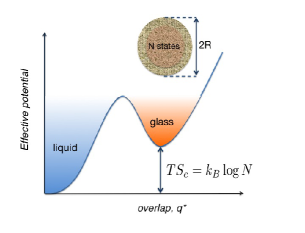
Figure 4: Mean-field theory description of the glassy states introduced the concept of an effective potential. Effective potential is designed to describe the transition between the non-ergodic glassy states and ergodic liquid.

The physically intuitive analogy between effective temperature, mean energy, $\overline{F}$ and configurational entropy to  thermodynamic relations, Eq. (33), suggest that one should analyze the corresponding configurational heat capacity

$$C_{c}=T_{\mathrm{eff}}\frac{\partial\overline{S_{c}}}{\partial T_{\mathrm{eff}}}=-m\frac{\partial\overline{S_{c}}}{\partial m}.$$ (34)

Using the distribution function Eq. (25) we find, as expected, that $C_{c}$ is a measure of the fluctuations of the energy and configurational entropy of glassy states.  We obtain for the configurational heat capacity

$$C_{c}=\frac{\overline{\left(\delta F\right)^{2}}}{T_{\mathrm{eff}}^{2}}\ =\overline{\left(\delta S_{c}\right)^{2}}.$$ (35)

where $\overline{\left(\delta F\right)^{2}}=\overline{F^{2}}-\overline{F}^{2}$ and $\overline{\left(\delta S_{c}\right)^{2}}=\overline{S_{c}^{2}}-\overline{S_{c}}^{2}$. Here the mean values $\overline{F}$ and $\overline{S_{c}}$ are determined by Eq. (33). The fluctuations of the configurational entropy and frozen state energy are then determined by

$$\overline{S_{c}^{2}}=\int D\psi P\left[\psi\right]\log^{2}P\left[\psi\right]$$ (36)

and

$$\overline{F^{2}}=\int D\psi P\left[\psi\right]F\left[\psi\right]^{2},$$ (37)

respectively. Both quantities can be expressed within the replica formalism in terms of a second derivative of $F\left(m\right)$ with respect to $m$. For example it follows:

$$\frac{\partial^{2}}{\partial m^{2}}mF\left(m\right)=-\frac{1}{T}\left(\overline{F^{2}}-\overline{F}^{2}\right).$$ (38)

It is then easy to show that Eq. (35) holds. With the introduction of the configurational heat capacity into the formalism we have a measure for the deviations of the number of metastable states from their mean value. The analogy of these results to the usual fluctuation theory of thermodynamic variables Landau further suggests that $C_{c}$ also determines fluctuations of the effective temperature with mean square deviation:

$$\overline{\left(\delta T_{\mathrm{eff}}\right)^{2}}=T_{\mathrm{eff}}^{2}/C_{c}.$$ (39)

Since $C_{c}$ is extensive, fluctuations of intensive variables, like $T_{\mathrm{eff}}$, or densities, like $s_{c}=S_{c}/V$, vanish for infinite systems. However, they become relevant if one considers finite subsystems or small droplets. In the context of glasses this aspect was first discussed in Ref. Donth .

If the replica theory is marginally stable, i.e. the lowest eigenvalue of the fluctuation spectrum beyond mean field solution vanishes, it was shown in Ref. WSW03 that $T_{\mathrm{eff}}$ agrees with the result obtained from the generalized fluctuation-dissipation theorem in the dynamic description of mean field glasses CK93 . Typically, the assumption of marginality is appropriate for early times right after a rapid quench from high temperatures.  In this case $T_{\mathrm{eff}}>T$ for $T<T_{A}$, i.e. the distribution function of the metastable states is not in equilibrium on the time scales where mode coupling theory or the requirement for marginal stability applies. Above the Kauzmann temperature it is however possible to consider the situation where $T_{\mathrm{eff}}=T$, i.e. where the distribution of metastable states has equilibrated with the external heat bath of the system. Since we are interested in the restoration of ergodicity for $T_{K}<T<T_{A}$ we use $T_{\mathrm{eff}}=T$. Below the Kauzmann temperature the assumption $T_{\mathrm{eff}}=T$ cannot be made any longer as it implies a negative configurational entropy, inconsistent with the definition Eq. (27). It implies that the glass transition is now inevitable even if one could wait for arbitrarily long times. While this is likely an idealization of mean field theory, it demonstrates that the ageing behavior below and above the Kauzman temperature are very distinct.

III.2 Dynamical interpretation of the replica approach

Ultimately, glass formation is a dynamic phenomenon. It is therefore useful and illustrative to offer a dynamical interpretation of the replica formalism of Ref. Mon95 . Below we will provide a qualitative set of arguments. A detailed and quantitative derivation of the formalism, based on the dynamic theory of glassy systems by Kurchan and Cugliandolo CK93 , is given in Ref. WSW04 .

Consider a system characterized by a field variable $\varphi\left(\mathbf{x},t\right)$. Let us assume that certain field configurations evolve extremely slowly, and equilibrate at a much later times than others. In terms of particle coordinates, a natural choice for slow and fast variables would be the fiducial position $\mathbf{R}_{i}\left(t\right)$ and the harmonic vibrations $\mathbf{u}_{i}\left(t\right)$, according to $\mathbf{x}_{i}\left(t\right)=$ $\mathbf{R}_{i}\left(t\right)+\mathbf{u}_{i}\left(t\right)$. In our field theoretic description we assume that slow field configurations are characterized by $\psi\left(\mathbf{x},t\right)$ while we continue to refer to fast configurations as $\varphi\left(\mathbf{x},t\right)$. Let the dynamics of the fast degrees of freedom be governed by the Langevin equation

$$\Gamma\frac{\partial\varphi\left(\mathbf{x},t\right)}{\partial t}=-\frac{\delta\mathcal{S}\left(\varphi,\psi\right)}{\delta\varphi\left(x,t\right)}+\eta\left(x,t\right),$$ (40)

where

$$\mathcal{S}\left(\varphi,\psi\right)=\mathcal{S}\left[\varphi\right]\ +\frac{g}{2}\int dx\left(\varphi\left(x\right)-\psi\left(x\right)\right)^{2}$$ (41)

contains a weak coupling ($g\ll 1$) between fast and slow degrees of freedom, just like in the replica approach discussed above. Fast variables $\ \varphi\left(\mathbf{x},t\right)$ are subject to white noise with temperature $T$

$$\left\langle\eta\left(\mathbf{x},t\right)\eta\left(\mathbf{x}^{\prime},t^{\prime}\right)\right\rangle=2\Gamma T\delta\left(\mathbf{x}-\mathbf{x}^{\prime}\right)\delta\left(t-t^{\prime}\right).$$ (42)

The equilibrium distribution function for fixed $\psi$ is then

$$p\left[\varphi|\psi\right]=\frac{1}{Z\left[\psi\right]}\exp\left(-\beta\mathcal{S}\left(\varphi,\psi\right)\right)$$ (43)

where $Z\left[\psi\right]=\int D\varphi\exp\left(-\beta\mathcal{S}\left[\varphi,\psi\right]\right)$.  Next we assume that the dynamics of the slow degrees of freedom is then governed by

$$\Gamma_{s}\frac{\partial\psi\left(\mathbf{x},t\right)}{\partial t}=-\frac{\delta F\left[\psi\right]}{\delta\psi\left(x,t\right)}+\eta_{s}\left(x,t\right).$$ (44)

with $F\left[\psi\right]=-T\log Z\left[\psi\right]$. Thus, during the entire dynamics of the slow degrees of freedom, the fast modes are assumed to be in equilibrium already. It is important to assume different noise for the slow variables $\psi\left(x,t\right)$ and for the fast variables $\varphi\left(x,t\right)$.  The variables $\psi\left(\mathbf{x},t\right)$ will, in general, not equilibrate with temperature $T$, but may be characterized by an effective temperature $T_{\mathrm{eff}}\geq T$, i.e. we write:

$$\left\langle\eta_{s}\left(x,t\right)\eta_{s}\left(x^{\prime},t^{\prime}\right)\right\rangle=2\Gamma_{s}T_{\mathrm{eff}}\delta\left(x-x^{\prime}\right)\delta\left(t-t^{\prime}\right)$$ (45)

Then, the stationary probability distribution for $\psi$ is

$$p\left[\psi\right]=\frac{1}{Z}\exp\left(-\beta_{\mathrm{eff}}F\left[\psi\right]\right)=\frac{Z\left[\psi\right]^{m}}{Z}$$ (46)

with $m=T/T_{\mathrm{eff}}$. The joint distribution of $\varphi$ and $\psi$ can now be written as $p\left[\varphi,\psi\right]=p\left[\psi\right]p\left[\varphi|\psi\right]$. It is straightforward to show that this distribution gives results identical to the replica approach. Above the Kauzmann temperature, $T_{K}$, equilibration of the slow variables is still possible and $T$ approaches $T_{\mathrm{eff}}$, i.e. $m\rightarrow 1$

IV Glass formation in uniformly frustrated systems

To gain detailed insight into the possibility of glass formation, we now go back to our model described by and analyze the problem (4) with $W\left(\varphi\right)=\frac{u_{4}}{4}\varphi^{4}$ analytically within the self consistent screening approximation (SCSA) SCSA , an approximate treatment that is controlled by an expansion in $1/N$, where $N$ is the number of components of $\varphi$, see Ref. SWW00 .

The free energy $F(m)$ of the replicated Hamiltonian is given in terms of the regular correlation function $G(q)$ and the correlation function $F(q)\equiv\langle\varphi^{a}(q)\varphi^{b}(-q)\rangle$ for $a\neq b$, i.e. between the fields in different replicas. The latter corresponds to the Edward-Anderson parameter signaling a glassy state. For a system in the universality class of the random first order transition we expect that below a temperature $T_{A\text{ }}$ the system establishes an exponentially large number of metastable states and long time correlations, characterized by the correlation function $F\left(\mathbf{x,x}^{\prime}\right)=T^{-1}\lim_{t\rightarrow\infty}\left\langle\varphi\left(\mathbf{x},t\right)\varphi\left(\mathbf{x}^{\prime},0\right)\right\rangle$. These long time correlations occur even though no state with actual long range spatial order exists.

Within the SCSA, the relevant part of the free energy $F(m)$ is:

$$F(m)=-\frac{T}{m}(\mathrm{Tr}\ln\mathcal{G}^{-1}+\mathrm{Tr}\ln\mathcal{D}^{-1}),$$ (47)

which determines the configurational entropy $S_{c}=\left.\frac{1}{T}\frac{d\mathcal{F}(m)}{dm}\right|_{m=1}$. Here,

$$\mathcal{G}\equiv(G-F)\mathbf{I}+F\mathbf{E}$$ (48)

is the correlation function matrix with $\mathbf{I}_{ab}=\delta_{ab}$ and $\mathbf{E}_{ab}=1$. The symbol Tr in Eq. (47) includes the trace of the replica space and the momentum integration. The matrix $\mathcal{D}$ is related to $\mathcal{G}$ via

$$\mathcal{D}^{-1}=(uT)^{-1}\mathbf{I}+\Pi,$$ (49)

where

$$\Pi=(G\otimes G-F\otimes F)\mathbf{I}+(F\otimes F)\mathbf{E}$$ (50)

is the generalized polarization matrix. The symbol $\otimes$ denotes a convolution in Fourier space. The replicated Schwinger-Dyson equation can be written as

$$\mathcal{G}^{-1}=G_{H}^{-1}\mathbf{I}+\Sigma,$$ (51)

where $\Sigma$ is the self-energy matrix and $G_{H}\left(k\right)$ the Hartree correlation function of Eq. (11).

Within the SCSA the self-energy has diagonal elements $\Sigma_{G}=2G\otimes D_{G}$ and off diagonal elements $\Sigma_{F}=2F\otimes D_{F}$ in replica space, where $D_{G}$ and $D_{F}$ being, respectively the diagonal and off-diagonal elements of $\mathcal{D}$. These equations form a closed set of self-consistent equations which enable us to solve for $G$ and $F$, and then determine the configurational entropy. To evaluate $F(m)$ we use the fact that a matrix of the form $A_{ab}=\left(a-b\right)\delta_{ab}+b$ has $m-1$ degenerate eigenvalues $a_{i}=a-b$ where $i=1,m-1$ and and one eigenvalue $a_{m}=a+\left(m-1\right)b$. This yields

$$\mathrm{Tr}\log A=\sum_{i=1}^{m}\int\frac{d^{d}k}{\left(2\pi\right)^{d}}\log a_{i}$$ (52)

This result allows us to evaluate $F\left(m\right)$ of Eq. (47). Performing the derivative of the resulting expression with respect to $m$ then yields the configurational entropy

$$S_{\mathrm{c}}=\int\frac{d^{d}q}{\left(2\pi\right)^{d}}\left\{s\left[\frac{F}{G}\right]-s\left[\frac{F\otimes F}{(u_{4}T)^{-1}+G\otimes G}\right]\right\},$$ (53)

were, $s[x]\equiv-x-\ln(1-x)$.

The analysis of these coupled equations reveals that the self energies $\Sigma_{G}$ and $\Sigma_{F}$ are only weakly momentum dependent. Then the impact of $\Sigma_{G}$ is solely to renormalize the correlation length $\xi$. However, the emergence of $\Sigma_{F}$ leads to a qualitative change. Dimensional analysis reveals that $\Sigma_{F}$ is an inverse length squared, which motivates one to introduce the Lindemann length $\lambda$ of the glass via $\lambda^{-2}=-A_{0}\Sigma_{F}$. An interpretation of this length scale in terms of slow defect motion in a stripe glasses was given in Ref. WSW03 . By inspection of the Dyson equation and using the fact that $G\left(k\right)$ is strongly peaked at the modulation wave number $k_{0}$ one finds for $k\sim k_{0}$ that

$$F\left(k_{0}\right)\lesssim G\left(k_{0}\right).$$ (54)

$G\left(k\right)$ vanishes rapidly away from the peak (as does $\Sigma_{F}(k_{0})G\left(k_{0}\right))$) and it follows from the same equation, 51, that for large $\left|k-k_{0}\right|$ holds:  

$$F\left(k\right)\simeq-\Sigma_{F}\left(k_{0}\right)G^{2}\left(k\right).$$ (55)

If a solution for $F$ exists, it is going to be a peaked at $k_{0}$, but smaller and narrower than $G$. Consequently, if a stripe glass occurs, the long time limit of the correlation function is not just a slightly rescaled version of the instantaneous correlation function, but it is multiplied by a $k$ dependent function that leads to a qualitatively different behavior for different momenta. Once a glassy state is formed, configurations which contribute to the peaks of $G\left(k\right)$ and $F\left(k\right)$, i.e. almost perfect stripe configurations, are almost unchanged even after long times. Close to $k_{0}$, $F\left(k\right)\,$ is solely reduced by some momentum independent Debye-Waller factor $\exp\left(-D\right)=F\left(k_{0}\right)/G\left(k_{0}\right)$. On the other hand, configurations which form the tails of $G\left(k\right)$, i.e. defects and imperfections of the stripe pattern, disappear after a long time since now $F\left(k\right)\ll G\left(k\right)$. The ratio of both functions is now strongly momentum dependent. $F\left(k\right)$ becomes sharper than $G\left(k\right)$ because local defects got healed in time. The length scale that determines the transition between these two regimes is the length $\lambda$.  This length can therefore be associated with the allowed generalized vibrational motions in a potential minima of the complex energy landscape of the system. In analogy with structural glasses we therefore call $\lambda$ the Lindemann length of the stripe glass.

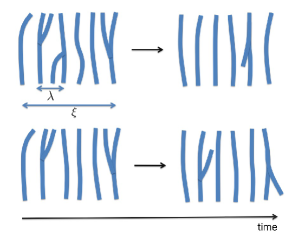
Figure 5: Schematic presentation of the defects wandering in structural glasses. Here $\lambda$ is an average distance over which the defects are manage to wander (Lindemann length) and $\xi$ is the correlation length (see text). Upper panel illustrates the situation when defects are relatively close to each other so that they disappear with time and system effectively heals itself. Bottom panel depict the opposite situation when wandering of the defects does not produce healing since they are on distances $l>\lambda$ from each other (see Ref. SWW00 for details.)

For our subsequent analysis we introduce the dimensionless quantity $Q$ via

$$\Sigma_{F}=-Q\frac{q_{0}^{2}}{A_{0}},$$ (56)

i.e. $\lambda^{-2}=Qq_{0}^{2}$. We are now in a position to perform the momentum integration and evaluate the configurational entropy as function of $Q$. It follows that

$$S_{c}\left(Q\right)=Vk_{0}^{d}K_{d}\left[\frac{1}{\xi q_{0}}\frac{z^{2}}{(1-z)}+\frac{2}{\pi}\left(z^{2}+\log\left(1-z^{2}\right)\right)\right]$$ (57)

where

$$z\left(Q\right)=1-\frac{1}{\sqrt{1+Q\xi^{2}q_{0}^{2}}}.$$ (58)

In Fig. 6 we show our results for $S_{c}\left(Q\right)$ for different values of $\varepsilon\equiv\xi q_{0}$. A self consistent solution of the above set of coupled equations corresponds to finding stationary points $Q^{\ast}$ with

$$\left.\partial S_{c}/\partial Q\right|_{Q=Q^{\ast}}=0.$$ (59)

$Q^{\ast}=0$ is always a solution with $S_{c}\left(0\right)=0$. In addition there is a locally stable solution for $\varepsilon>\varepsilon_{A}=11.770574$ with configurational entropy given as $S_{c}\left(Q_{A}^{\ast}\right)=Vk_{0}^{d}K_{d}\times 0.0220247$ and $Q_{A}^{\ast}=Q^{\ast}\left(\varepsilon_{A}\right)=0.0625528$. The configurational entropy at the metastable maximum vanishes at $\varepsilon=\varepsilon_{K}=13.169625$ with $Q_{K}^{\ast}=0.134271$.  This is the behavior that is generally expected in a system a with random first order transition. Upon lowering the temperature the ergodic, liquid like state becomes more and more correlated, i.e. the correlation length growths. Once $\xi$ reaches a threshold value $\xi_{A}=\frac{\varepsilon_{A}}{2\pi}l_{0}\simeq 1.\,\allowbreak 87l_{0}$ about twice the typical length scale for field modulations $l_{0}=2\pi/q_{0}$, glassy dynamics sets in as consequence of an emergence of exponentially many states. The Kauzman temperature is reached once the liquid state correlation length grows even further and becomes equal to $\xi_{K}=\frac{\varepsilon_{K}}{2\pi}l_{0}\simeq 2.1l_{0}$.

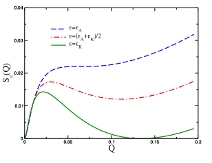
Figure 6: Plot of the configurational entropy $S_{c}(Q)$ as a function of the dimensionless parameter $Q=(1/\lambda q_{0})^{2}$, Eq. (4.10) for different values of another parameter $\varepsilon=\xi q_{0}$. It is instructive to compare this plot with the schematic plot of Fig. 4.

It is also interesting to analyze the penalty for a spatially varying overlap $Q\to Q({\mathbf{x}})$. This will be essential for the Landau expansion and the droplet arguments that follow below. Performing a gradient expansion of the replica free energy yields the correction

$$\delta F(m)=-\frac{a_{0}^{2}}{2}(m-1)T\int d^{d}x\left({\vec{\nabla}}Q\right)^{2},$$ (60)

where

$$a_{0}^{2}=\frac{k_{0}^{4}}{A_{0}^{2}}\lim\limits_{q\to 0}\frac{1}{q^{2}}\int\frac{d^{d}k}{(2\pi)^{d}}\left[G(k)G(k+q)-G^{2}(k)\right]$$ (61)

The prefactor $k_{0}^{4}/A_{0}^{2}$ appears from our definition for $Q$ (56). For $d=3$ and $\tau=1$ the integration can be performed exactly with the following result SWW00 :

$$a_{0}^{2}=\frac{k_{0}}{48\pi}(\xi k_{0})^{5}.$$ (62)

As was anticipated in Ref. SWW00 , the penalty for a spatial deformation becomes small as $k_{0}\to 0$, i.e. in the limit where the modulation length is very large. Note that at $T=T_{A}$ or $T=T_{K}$, the dimensionless product $\xi k_{0}$ is independent of $k_{0}$, i.e. varying the characteristic scale yields $a_{0}(T_{A})\propto k_{0}^{1/2}$.

Thus, we analyzed an analytically treatable example for a random first order transition which enabled us to identify the underlying physical mechanism for glassiness in a uniformly frustrated system. Once equilibrium correlations are sufficiently strong and the stripe liquid - stripe solid transition is kinematically inaccessible, the system is governed by slow glassy dynamics. At this point a Lindemann length, $\lambda$, emerges, which is a length scale over which imperfections of the stripe pattern manage to wander, Fig. 5. Defects of the perfectly ordered state are still abundant as the healing length is finite, i.e. the system enters a random solid state. Local order is however established. This may not be identical to the most stable crystalline, i.e. long ranged ordered, configuration, but rather correspond to configurations that are occurring with high weight close to the spinodal of the system. In the context of supercooled liquids, the natural analog of such locally correlated configuration are icosahedral or body centered cubic short range order.

Computer simulations on the model discussed above with $u_{3}=0$, suggest that the nucleation barriers of the crystalline state are rather low Geissler04 . However, the inclusion of asymmetric terms in the interaction potential ($u_{3}\neq 0$) will likely strengthen first order transitions to a crystalline state and enhance the nucleation barriers. This behavior was analyzed in Refs. WSW04 ; Zhang06 ; Wu09 .

V Replica Landau Theory

The analysis of the previous section demonstrated that  uniformly frustrated systems undergo self generated glass transitions with an entropy crisis, of the random first order transition universality class. These calculations are on the mean field level and ignore issues related to dynamical heterogeneity, i.e. variations in the typical time scales in spatially nearby regions. The relevance of such effect is already evident from the fact that fluctuations in the heat capacity become important in finite regions, as shown above. To capture these phenomena we need to go beyond the mean field level and include droplet formations. Droplets are not regions with different values of the field $\varphi\left(\mathbf{r}\right)$ that underlies our analysis. Instead, by droplets we mean a spatial variation of the Lindemann length, i.e. of the parameter $Q$ used above to characterize the overlap between configurations at distant times. Thus, it is useful to consider instead of $Q$ a dynamic field $Q_{ab}\left(\mathbf{r}\right)$ that generates the replica partition function, i.e.

$$Z\left(m\right)=\int DQ\exp\left(-\beta H_{\mathrm{eff}}\left[Q\right]\right).$$ (63)

The mean field solution of this problem is then determined by $\delta H_{\mathrm{eff}}\left[Q\right]/\delta Q_{ab}=0$ with the Ansatz

$$Q_{ab}=Q^{\ast}\left(1-\delta_{ab}\right)$$ (64)

with $Q^{\ast}$ playing the exact same role as the corresponding quantity determined by the condition Eq. (59) in the previous section.

Formally $H_{\mathrm{eff}}\left[Q\right]$ can be obtained from the field theory discussed above by multiplying $Z\left(m\right)$ of Eq. (32) by unity

$$\begin{split}1=&\int D\mu\prod\limits_{\mathbf{x,x}^{\prime},ab}\delta\left(\mu_{ab}\left(\mathbf{x,x}^{\prime}\right)-\varphi^{a}(\mathbf{x})\varphi^{b}(\mathbf{x}^{\prime})\right)=\\ =&\int\limits_{-i\infty}^{i\infty}DQ\int D\mu\exp\left\{-\int_{\mathbf{x,x}^{\prime}}\sum_{ab}Q_{ab}\left(\mathbf{x,x}^{\prime}\right)\times\right.\\ &\left.\times\left[\mu_{ab}\left(\mathbf{x,x}^{\prime}\right)-\varphi^{a}(\mathbf{x})\varphi^{b}(\mathbf{x}^{\prime})\right]\right\}\end{split}$$ (65)

and switch the order of integration. Then we find

$$\begin{split}&e^{-H_{\mathrm{eff}}\left[Q\right]}=\int D\mu D^{m}\varphi e^{-\sum_{a=1}^{m}\beta\mathcal{H}\left[\varphi^{a}\right]}\times\\ &\times e^{-\sum_{a,b=1}^{m}\int_{\mathbf{x,x}^{\prime}}Q_{ab}(\mathbf{x,x}^{\prime})\left(\mu_{ab}(\mathbf{x,x}^{\prime})-\varphi^{a}(\mathbf{x})\varphi^{b}(\mathbf{x}^{\prime})\right)}.\end{split}$$ (66)

We consider the Fourier transform of $Q_{ab}\left(\mathbf{x,x}^{\prime}\right)$ with respect to the relative coordinates $\mathbf{x-x}^{\prime}$ and approximate it by its value at $k=k_{0}$. This is consistent with our finding that the self energies of the mean field theory depend only weakly on momentum. We do however include the dependence on the center of gravity coordinate to analyze spatially varying overlaps between distant configurations, yielding $Q_{ab}\left(\mathbf{x}\right)$.

In order to keep our calculation transparent we will not analyze the model discussed for uniformly frustrated systems, but instead start from a simpler Landau theory that is in the same universality class Gross85 ; Dzero05 :

$$H_{\mathrm{eff}}\left[Q\right]=E_{0}\sum_{a,b}\int\frac{d^{3}r}{a_{0}^{3}}\left(h\left[Q_{ab}\right]-\frac{u}{3}\sum_{c}Q_{ab}Q_{bc}Q_{ca}\ \right)$$ (67)

with

$$h\left[Q_{ab}\right]=\frac{a_{0}^{2}}{2}\left(\nabla Q_{ab}\right)^{2}+\frac{t}{2}Q_{ab}^{2}-\frac{u+w}{3}Q_{ab}^{3}+\frac{y}{4}Q_{ab}^{4}$$ (68)

and replica index $a$,$b=1,\ldots,m$. $\ a_{0}$ is a length scale of the order of the first peak in the radial distribution function of the liquid and $E_{0}$ is a typical energy of the problem that determines the absolute value of $T\overline{s_{c}}$. In addition the problem is determined by the dimensionless variables $t$, $u$, $w$ and $y$, which are in principle all temperature dependent. We assume that the primary $T$-dependence is that of the quadratic term, where $t=\frac{T-T_{0}}{E_{0}}$. In what follows we further simplify the notation and measure all energies in units of $E_{0}$ and all length scales in units of $a_{0}$. Formally, Eqs. (67)  and (68) can be motivated as the Taylor expansion of  the free energy $F\left[m\right]$ with respect to $\Sigma_{ab}$.  In practice, the explicit Taylor expansions of more microscopic models do not yield quantitatively reliable results. For example, the Taylor expansion of Eq. (57) poorly reproduces the behavior in the glassy regime. Still, the simple Landau expansion of Eqs. (67)  and (68) allows us to gain key insights that enable us to investigate the more general case. In particular, we will demonstrate that the replica instanton theory can easily be generalized to the more complex stripe glass model.

The mean field analysis of the model Hamiltonian Eqs. (67) and (68) is straightforward. Inserting the Ansatz Eq. (64) into $H_{\mathrm{eff}}\left[Q\right]$ and minimizing w.r.t $Q$ yields $Q^{\ast}=0$ or

$$Q^{\ast}\left(t\right)=\ \frac{w+\sqrt{w^{2}-4ty}}{2y}.$$ (69)

Nontrivial solutions exits for $t<t_{A}=\frac{w^{2}}{4y}$ with $Q_{A}^{\ast}=Q^{\ast}\left(t_{A}\right)=\frac{w}{2y}$, which determines the mode coupling temperature $T_{A}=t_{A}E_{0}+T_{0}$. Inserting $Q^{\ast}$ of Eq. (69) into $H_{\mathrm{eff}}\left[Q\right]$ yields at the saddle point $F\left(m\right)=H_{\mathrm{eff}}\left[Q\right]$ for the replica free energy, which yields:

$$\frac{F\left(m\right)}{V\left(m-1\right)}=\frac{t}{2}Q^{\ast 2}-\frac{w+u\left(m-1\right)}{3}Q^{\ast 3}+\frac{y}{4}Q^{\ast 4}.$$ (70)

The configurational entropy, as determined by $S_{c}=\left.\frac{1}{T}\frac{\partial}{\partial m}F\left(m\right)\right|_{m\rightarrow 1}$ is given by

$$S_{c}\left(Q\right)=\frac{V}{T}\left(\frac{t}{2}Q^{2}-\frac{w}{3}Q^{3}+\frac{y}{4}Q^{4}\right).$$ (71)

The stationary points of $S_{c}\left(Q\right)$ are given by $Q^{\ast}$ of Eq.69. Inserting $Q^{\ast}$ yields that $S_{c}$ vanishes at $t_{K}=\frac{2w^{2}}{9y}$ with $Q_{K}^{\ast}=\frac{2w}{3y}$. Close to $t_{K}$ it follows that

$$S_{c}\simeq V\frac{t_{K}}{y}\left(\frac{t-t_{K}}{T_{K}}\right)\propto V\frac{T-T_{K}}{T_{K}}$$ (72)

as expected. At $t_{A}$ one finds $T_{A}S_{c}\left(T_{A}\right)=V\frac{w^{4}}{192y^{3}}$.     For the configurational heat capacity follows

$$C_{c}\ =\frac{2V}{T}\ \left(\frac{t}{2}Q^{\ast 2}-\frac{w+u}{3}Q^{\ast 3}+\frac{y}{4}Q^{\ast 4}\right)$$ (73)

It holds at $C_{c}\left(T_{K}\right)=\frac{Vu}{T_{K}}\frac{2}{3}\left(\frac{2w}{3y}\right)^{3}$ and we can write

$$S_{c}\simeq\frac{w}{4u}C_{c}\left(t_{K}\right)\ \frac{t-t_{K}}{t_{K}}.$$ (74)

Thus, we see that the main findings of the model calculations are reproduced by the simple Landau expansion, Eqs. (67) and (68). They will now be used as starting point for our analysis of dynamical heterogeneity in form of a replica instanton theory.

VI Replica instantons and entropic droplets

At the mean field level a glass at $T<T_{A}$ is frozen in one of many metastable states. $Q^{\ast}$ then characterizes the overlap between configurations at distant times. The free energy of such a frozen state is higher by $TS_{c}$ compared to the ergodic liquid state that is characterized by $Q^{\ast}=0$. Thus, for $T_{K}<T<T_{A}$ the mean field glass is locally stable. Local stability also follows from the fact that the lowest eigenvalue of the fluctuation matrix $\delta^{2}H/\delta Q_{ab}\left(\mathbf{x}\right)\delta Q_{cd}\left(\mathbf{x}^{\prime}\right)$ is positive for $T_{K}\leq T<T_{A}$ and vanishes at $T=T_{A}$, see Ref. Dzero05 . The $Q$-dependence of $S_{c}\left(Q\right)$ shown in Fig. 6 suggests that the decay modes for the frozen state are droplet excitations, similar to the nucleation of an unstable phase close to a first order transition. This situation was analyzed in  Ref. Franz05-1 ; Dzero05 . In agreement with the RFOT theory KTW89 , the driving force for nucleation is the configurational entropy, leading to the notion of entropic droplets. The formal approach to analyze entropic droplets is performed in terms of the effective potential approach of Refs. Franz95 ; Franz97 ; Barrat97 . We used this technique to formulate a replica instanton and barrier fluctuation theory in Refs. Dzero05 ; Dzero09 . In what follows we use a slightly simpler approach that yields essentially the same results, but is physically significantly more transparent.

As can be motivated by the more general effective potential approach of Refs. Franz95 ; Franz97 ; Barrat97 , instanton solutions for entropic droplets can be determined from

$$\frac{\delta H\left[Q\right]}{\delta Q_{ab}\left(\mathbf{x}\right)}=0,$$ (75)

where we allow for spatial variations of the overlap $Q_{ab}\left(\mathbf{r}\right)=Q\left(\mathbf{r}\right)\left(\delta_{ab}-1\right)$. This yields the following nonlinear equation for $Q\left(\mathbf{r}\right)$:

$$\nabla^{2}Q\left(\mathbf{r}\right)=\frac{ds_{c}\left(Q\left(\mathbf{r}\right)\right)}{dQ\left(\mathbf{r}\right)},$$ (76)

with configurational entropy density $s_{c}\left(Q\right)=S_{c}\left(Q\right)/V$. In case of the Landau expansion we use $S_{c}\left(Q\right)$ of Eq. (71), while for the stripe glass approach we start from Eq. (57). We will first analyze the simpler case of the Landau theory. Then Eq. (76) admits an exact solution in the  thin wall limit $R\gg\xi$:

$$Q(x)=q^{\ast}+\sqrt{\frac{2}{y\xi^{2}}}\left[\text{th}\left(\frac{x}{\xi}-z_{0}\right)-\text{th}\left(\frac{x}{\xi}+z_{0}\right)\right],$$ (77)

where the integration constant $z_{0}$ is a function of $t,w$ and $y$. $R$ is the droplet radius and $\xi$ is the interface width given by

$$\xi=\frac{4a_{0}}{\sqrt{3y(2Q^{\ast}-Q_{K}^{\ast})^{2}-6t_{K}+4t}}.$$ (78)

Inserting the solution Eq. (77) into the expression into $H\left[Q\right]$ we calculate the value of the mean barrier. The latter is determined by optimizing the energy gain due to creation of a droplet and energy loss due to the surface formation. As a result for the mean barrier we find (reintroducing the energy scale $E_{0}$ and length scale $a_{0}$)

$$\overline{F^{\ddagger}}=E_{0}\frac{32\pi a_{0}}{9y\xi^{3}}R^{2},$$ (79)

The droplet radius

$$R=\frac{64a_{0}^{4}}{3y^{2}q^{\ast 3}(q_{K}^{\ast}-q^{\ast}\left(t\right))\xi^{3}}$$ (80)

is determined from the balance between the interface tension and the entropic driving force for nucleation. Furthermore, $q_{K}^{\ast}\equiv q^{\ast}(t=t_{K})$ is the order parameter at the Kauzmann temperature. When temperature approaches the $T_{K}$ the radius of the droplet as well as the mean barrier diverge. One finds $\lim\limits_{t\rightarrow t_{K}}\overline{F^{\ddagger}}\propto(t-t_{K})^{-2}$ and $\lim\limits_{t\rightarrow t_{K}}R\propto(t-t_{K})^{-1}$. Since the droplet interface $\xi$ remains finite as $t\rightarrow t_{K}$, the thin wall approximation is well justified close to the Kauzman temperature. On the other hand, $R$ and $\xi$ become comparable for temperatures close to $T_{A}$ and the thin wall approximation breaks down. Combining $R\propto(t-t_{K})^{-1}$ and $s_{c}\propto(t-t_{K})$, we obtain $\nu=1$ for the exponent that relates the droplet size $R$ and the configurational entropy density: $R\propto s_{c}^{-\nu}$.

Close to $t_{K}$ follows  $\sigma\left(t\right)\simeq\sigma_{K}\left(1-\frac{21}{\ 2}\left(\frac{t-t_{K}}{t_{K}}\right)\right)$ with $\sigma_{K}=\frac{4a_{0}}{27\sqrt{15}}\frac{w^{3}}{y^{5/2}}.$ The critical droplet nucleation radius is $R=2\sigma/s_{c}$ yielding the barrier

$$\overline{F^{\ddagger}}=\frac{16\pi\sigma^{3}}{3s_{c}^{2}}$$ (81)

for the nucleation of entropic droplets. This leads to a mean relaxation time of

$$\overline{\tau}=\tau_{0}\exp\left(\frac{\overline{F^{\ddagger}}}{k_{B}T}\right).$$ (82)

It was pointed out in Ref. KTW89 that wetting effects of the interface alter the a relationship between droplet size and entropic driving force to $R\propto s_{c}^{-\nu}$ with exponent $\nu$. A renormalization of the droplet interface due to wetting of intermediate states on the droplet surface was shown to yield $\nu=2/d$ KTW89 , leading to $\overline{F^{\ddagger}}\propto Ts_{c}^{-1}$ and correspondingly to a Vogel-Fulcher law

$$\overline{\tau}=\tau_{0}\exp\left(\frac{DT_{K}}{T-T_{K}}\right)$$ (83)

for the mean relaxation time.

It is straightforward to analyze the more complex configurational entropy of the stripe glass problem. In this case the nonlinear instanton equation cannot be solved analytically. However we can make progress by performing a variational calculation for the droplet. The mean barrier is

$$\overline{F^{\ddagger}}=H_{\mathrm{eff}}\left[Q\left(\mathbf{x}\right)\right]-S_{c}\left(Q^{\ast}\right),$$ (84)

where $Q\left(\mathbf{x}\right)$ is a localized instanton solution which differs from $Q^{\ast}$ in a finite region. We make the trial ansatz:

$$Q\left(\mathbf{x}\right)=\left\{\begin{array}[]{cc}0&\left|\mathbf{x}\right|<R\\ Q^{\ast}\frac{\left|\mathbf{x}\right|-R}{l}&R<\left|\mathbf{x}\right|<R+l\\ Q^{\ast}&\left|\mathbf{x}\right|>R+l\end{array}\right.$$ (85)

and insert it into the above expression for $H_{\mathrm{eff}}\left[Q\left(\mathbf{x}\right)\right]$. We find

$$\overline{F^{\ddagger}}\left(R\right)=4\pi\sigma R^{2}-\frac{4\pi}{3}s_{c}\left(Q^{\ast}\right)R^{3}$$ (86)

with surface tension

$$\sigma=\frac{a_{0}^{2}Q^{\ast 2}}{2l}+lT\left[\int_{0}^{Q^{\ast}}s_{c}\left(Q\right)\frac{dQ}{Q^{\ast}}-s_{c}\left(Q^{\ast}\right)\right]$$ (87)

Minimizing with respect to the droplet wall thickness $l$ yields

$$l^{2}=\frac{1}{2}\frac{a_{0}^{2}Q^{\ast 3}}{\int_{0}^{Q^{\ast}}s_{c}\left(Q\right)dQ-s_{c}\left(Q^{\ast}\right)Q^{\ast}}$$ (88)

and correspondingly for the surface tension

$$\sigma=\sqrt{2}a_{0}Q^{\ast 1/2}\left(\int_{0}^{Q^{\ast}}s_{c}\left(Q\right)dQ-s_{c}\left(Q^{\ast}\right)Q^{\ast}\right)^{1/2}$$ (89)

Using the our result Eq. (57) for the configurational entropy as a function of $Q$ for the stripe glass problem in $d=3$ and for $\tau=1$ (i.e. with the long range Coulomb interaction $V({\mathbf{x}})$) and Eq. (62) for the gradient coefficient $a_{0}$, yields at $T_{K}$:

$$\sigma(T_{K})=C_{\sigma}T_{K}k_{0}^{2},$$ (90)

where $C_{\sigma}\simeq 3.45\times 10^{-2}$. Thus we see that the surface tension of entropic droplets vanishes in the limit $k_{0}\rightarrow 0$. For the wall thickness we obtain $l(T_{K})\simeq k_{0}^{-1}$.

Finally, we use our results for the surface tension to analyze the variation of the fragility $D$ in Eq. (83) as function of $k_{0}$. One finds

$$D=\frac{3\sigma^{2}}{T_{K}^{3}\left(\frac{dS_{c}}{dT}\right)_{T=T_{K}}}$$ (91)

which was further investigated in a numerical analysis of the stripe glass problem in Ref. Grousson2001 . This analysis led to $D(k_{0}\to 0)\to 0$. If we make the following estimate

$$\left(\frac{dS_{c}}{dT}\right)_{T=T_{K}}\simeq\frac{s_{c}(T_{A})}{T_{A}-T_{K}}$$ (92)

and neglect the dependence of $T_{A}-T_{K}$ on $k_{0}$, we find that $D\propto k_{0}$ in qualitative agreement with the results of Ref. Grousson2001 .

VI.1 barrier fluctuations

Numerous experiments on supercooled liquids are not only sensitive to the mean barrier, $\overline{F^{\ddagger}}$, but are able to measure the entire (broad) excitation spectrum in glasses Richert02 . Most notably, the broad peaks in the imaginary part of the dielectric function $\varepsilon^{\prime\prime}\left(\omega\right)$ are most naturally understood in terms of a distribution $g\left(\tau\right)$ of relaxation times,  such that

$$\varepsilon^{\prime\prime}\left(\omega\right)\propto\int d\tau g\left(\tau\right)\frac{\omega\tau}{1+\left(\omega\tau\right)^{2}}.$$ (93)

Similarly dynamical heterogeneity with spatially fluctuating relaxation times yields non-exponential (frequently stretched exponential) relaxation of the correlation function

$$\phi\left(t\right)=\int d\tau g\left(\tau\right)e^{-t/\tau},$$ (94)

Other effects that are most likely caused by a distribution of relaxation rates include the break down of the Stokes-Einstein relation $D=\frac{k_{B}T}{4\pi\eta L}$ between the diffusion coefficient $D$ of a particle of size $L$ and the viscosity $\eta$ Fujara92 ; Cicerone95 . These experiments call for a more detailed analysis of the fluctuations

$$\overline{\delta F^{\ddagger 2}}\equiv\overline{F^{\ddagger 2}}-\overline{F^{\ddagger}}^{2}$$ (95)

of the activation barriers and, more generally, of the distribution function $p\left(F^{\ddagger}\right)$ of barriers. The latter yields the distribution function of the relaxation times

$$g\left(\tau\right)=p\left(F^{\ddagger}\right)\frac{dF^{\ddagger}}{d\tau}$$ (96)

through $\tau\left(F^{\ddagger}\right)=\tau_{0}\exp\left(\frac{F^{\ddagger}}{k_{B}T}\right)$. For example, in case of a Gaussian distribution of barriers one obtains a broad, log-normal distribution of relaxation rates:

$$g\left(\tau\right)=\frac{1}{\tau\sqrt{2\pi\lambda}}\exp\left(-\frac{\log^{2}\left(\tau/\overline{\tau}\right)}{2\lambda}\right),$$ (97)

with

$$\lambda=\overline{\delta F^{\ddagger 2}}/\left(k_{B}T\right)^{2}$$ (98)

and $\overline{\tau}$ from Eq. (82). While the distribution, Eq. (97), does not yield a stretched exponential form for the correlation function, it can often be approximated by

$$\phi\left(t\right)\simeq\exp\left(-(t/\overline{\tau})^{\beta}\right)$$ (99)

with $\beta=\left(1+\lambda\right)^{-1/2}$. Furthermore, the study of higher order moments of $p\left(F^{\ddagger}\right)$ is important to determine whether the distribution is indeed Gaussian or more complicated.

In Ref. Dzero09 we used the replica formalism discussed here as well as the more elaborate replica method of formalism Refs. Franz95 ; Franz97 ; Barrat97 to determine higher order moments of the barrier distribution function. Using the ”thin wall” approximation for $Q({\mathbf{x}})$ given by Eq. (77)  we obtain for the second moment

$$\overline{\delta F^{\ddagger 2}}=A\left(R^{3}+\rho R^{2}\right),$$ (100)

where $R$ is the radius of the droplet where the explicit expressions for the coefficient $A$ and length $\rho$ are given in Ref. Dzero09 .  It is noteworthy that there is a surface contribution to the moment of the barrier fluctuations that is a consequence of correlations between droplet and homogeneous background with overlap $Q^{\ast}$. In Ref. Dzero09 it was also shown that the barrier distribution function $p\left(F^{\ddagger}\right)$ is Gaussian, at least if one considers the first six moments. The skewness of the actual barrier distribution measured in structural glasses is, in our view, an effect due to the interaction of spatially overlapping instantons.

VII Summary

To summarize, we have discussed several models of glassy systems where the randomness is self generated rather than induced by strong external factors. In particular, we applied the replica formalism developed for the spin glass systems to study the glass transition in the many-body systems at the presence of an arbitrary weak disorder. We employed the Landau theory to analyze the mean field glass transition using the saddle point approximation. We have also considered the energy fluctuations around the saddle point and evaluated the barrier height distribution.

- (1) C. A. Angel, in Proceedings of the XIV Sitges Conference, Complex Behavior of Glassy Systems, ed. by M. Rubi and C. Perez-Vicente, Lecture Notes in Physics, 492, p. 1 (1996).
- (2) C. A. Angell, J. Phys. Chem. Sol. 49, 863 (1988).
- (3) W. Götze, in Liquids, Freezing and Glass Transition, ed. J.-P. Hansen, D. Levesque and J. Zinn-Justin (North-Holland, Amsterdam, 1991), p. 287.
- (4) T. R. Kirkpatrick and D. Thirumalai, Phys. Rev. Lett. 58, 2091 (1987).
- (5) T. R. Kirkpatrick and P. G. Wolynes, Phys. Rev. A 35, 3072 (1987).
- (6) M. Kleman and J. F. Sadoc, J. Physique Lett. 40 L569 (1979), J. F. Sadoc, J. Phys. Lett. 44 L707 (1983); J. F. Sadoc and R. Mosseri, J. Physique 45 1025 (1984).
- (7) D. R. Nelson, Phys. Rev. Lett. 50 982 (1983); D. R. Nelson, Phys. Rev. B 28 5515 (1983); S. Sachdev and D. R. Nelson, Phys. Rev. Lett. 53 1947 (1984); S. Sachdev and D. R. Nelson, Phys. Rev. B 32 1480 (1985).
- (8) J. P. Sethna, Phys. Rev. Lett. 51 2198 91983); J. P. Sethna, Phys. Rev. B 31 6278 (1985).
- (9) F. Sausset, G. Tarjus and P. Viot, Journal of Statistical mechanics: Theory and Experiment, P04022 (2009).
- (10) D. Kivelson, S.A. Kivelson, X. Zhao, Z. Nussinov and G. Tarjus. Physica A 219, 27 (1995),
- (11) L. Chayes, V. J. Emery, S. A. Kivelson, Z. Nussinov and G. Tarjus, Physica A 225 129 (1996).
- (12) Z. Nussinov, J. Rudnick, S. A. Kivelson, and L. N. Chayes, Phys. Rev. Lett. 83 472 (1999).
- (13) M. Grousson, G. Tarjus, and P. Viot, Phys. Rev. E 65, 065103(R) (2002); M Grousson, G Tarjus and P Viot J. Phys.: Condens. Matter 14 1617 (2002).
- (14) M. Grousson, V. Krakoviack, G. Tarjus, and P. Viot, Phys. Rev. E 66, 026126 (2002).
- (15) G. Tarjus, S. A. Kivelson, Z. Nussinov and P. Viot, J. Phys.: Condens. Matter 17, R1143 (2005).
- (16) R. Monasson, Phys. Rev. Lett. 75, 2847 (1995).
- (17) M. Mezard and G. Parisi, Phys. Rev. Lett. 82, 747 (1999).
- (18) M. Mezard and G. Parisi, J. Chem. Phys. 111, 1076 (1999).
- (19) S. Franz and G. Parisi, J. Phys. I (France) 5, 1401 (1995).
- (20) T. R. Kirkpatrick and D. Thirumalai, and P. G. Wolynes, Phys. Rev. A 40, 1045 (1989).
- (21) X. Xia and P. G. Wolynes, Proc. Natl. Acad. Sci. 97, 2990 (2000).
- (22) X. Xia and P. G. Wolynes, Phys. Rev. Lett. 86, 5526 (2001).
- (23) V. Lubchenko, P. G. Wolynes, Phys. Rev. Lett. 87, 195901 (2001).
- (24) V. Lubchenko, P. G. Wolynes, Journ. of Chem. Phys. 121, 2852 (2004).
- (25) G. Biroli and J.-P. Bouchaud, Journ. of Chem. Phys., 121, 7347 (2004).
- (26) W. Kauzmann, Chemical Reviews 43,219 (1948).
- (27) J. S. Langer, Ann. Phys., NY 41, 108 (1967).
- (28) J.H. Cho, F.C. Chou, and D.C. Johnston, Phys. Rev. Lett. 70, 222 (1993).
- (29) J.M. Tranquada, J.J. Sternlieb, J.D. Axe, Y. Nakamura, and S. Uchida, Nature (London) 375, 561 (1995).
- (30) D. N. Argyriou, J. W. Lynn, R. Osborn, B. Campbell, J. F. Mitchell, U. Ruett, H. N. Bordallo, A. Wildes, C. D. Ling, Physical Review Letters 89, 036401 (2002).
- (31) A. J. Millis, Phys. Rev. B 53, 8434 (1996).
- (32) E. Dagotto, T. Hotta, and A. Moreo, Physics Reports (2001).
- (33) M.-H. Julien, F. Borsa, P. Carretta, M. Horvatic, C. Berthier, and C. T. Lin, Phys. Rev. Lett. 83, 604 (1999).
- (34) A. W. Hunt, P. M. Singer, K. R. Thurber, and T. Imai, Phys. Rev. Lett. 82, 4300 (1999).
- (35) N. J. Curro, P. C. Hammel, B. J. Suh, M. Hücker, B. Büchner, U. Ammerahl, and A. Revcolervschi, Phys. Rev. Lett. 85, 642 (2000).
- (36) J. Haase, R. Stern, C. T. Milling, C. P. Slichter, and D. G. Hinks, Physica C 341, 1727 (2000).
- (37) N. J. Curro, Journal of Physics and Chemistry of Solids 63, 2181(2002).
- (38) Ch. Niedermeyer, C. Bernhard, T. Blasius, A. Golnik, A. Moodenbaugh, and J. I. Budnik, Phys. Rev. Lett. 80, 3843 (1998).
- (39) C. Panagopoulos, J. L. Tallon, B. D. Rainford, T.Xiang, J. R. Cooper, and C. A. Scott, Phys. Rev. B 66, 064501 (2002).
- (40) J. Jaroszyński, T. Andrearczyk, G. Karczewski, J. Wróbel, T. Wojtowicz, Dragana Popović, and T. Dietl, Phys. Rev. B 76, 045322 (2007)
- (41) B. Spivak, S. A. Kivelson, Annals of Physics 321, 2071 (2006).
- (42) B. Spivak, S. V. Kravchenko, S. A. Kivelson, X. P. A. Gao, Rev. Mod. Phys. 82, 1743 (2010).
- (43) K.B. Cooper, M.P. Lilly, J.P. Eisenstein, P.N. Pfeiffer, and K.W. West, Phys. Rev. B 60, 11285 (1999).
- (44) S.A. Parameswaran, S.A. Kivelson, S.L. Sondhi, B.Z. Spivak, pre-print arXiv:1010.4908 (2010).
- (45) T. Garel and S. Doniach, Phys. Rev. B 26, 325 (1982); R. Allenspach and A. Bischof, Phys. Rev. Lett. 69, 3385 (1992).
- (46) P.G. deGennes and C. Taupin, J. Phys. Chem. 86, 2294 (1982); W.M. Gelbart and A. Ben Shaul, J. Phys. Chem. 100, 13169 (1996).
- (47) T. Ohta and K. Kawasaki, Macromolecule 19, 2621 (1986).
- (48) S. Bogdanovich and D. Popovic, Phys. Rev. Lett. 88, 236401 (2002).
- (49) J. Jaroszynki and D. Popovic, Phys. Rev. Lett. 96, 037403 (2006).
- (50) C. Panagopoulos and V. Dobrosavljevic, Phys. Rev. B72, 014536 (2002).
- (51) D. Dalidovich and P. Philips, Phys. Rev. Lett. 89, 27001 (2002).
- (52) V.J. Emery and S.A. Kivelson, Physica C 209, 597 (1993).
- (53) J. Schmalian and P.G. Wolynes, Phys. Rev. Lett. 85, 836 (2000).
- (54) H. Westfahl Jr., J. Schmalian, and P. G. Wolynes, Phys. Rev. B 64, 174203 (2001).
- (55) H. Westfahl Jr., J. Schmalian, and P. G. Wolynes, Phys. Rev. B 68, 134203 (2003).
- (56) S.Wu, J. Schmalian, G.Kotliar, and P. G. Wolynes, Phys. Rev. B 70, 024207 (2004).
- (57) P. Chandra, L.B. Ioffe, and D. Sherrington, Phys. Rev. B 58, R14669 (1998).
- (58) M. Dzero, J. Schmalian, and P. G. Wolynes, Phys. Rev. B 72, 100201 (2005).
- (59) M. Dzero, J. Schmalian, and P. G. Wolynes, Phys. Rev. B 80, 024204 (2009).
- (60) L. Leibler, Macromolecules 13, 1602 (1980).
- (61) G. H. Fredrickson and E. Helfand, J. Chem. Phys. 87, 697 (1987).
- (62) M. W. Deem and D. Chandler, Phys. Rev. E 49, 4268 (1994).
- (63) S. Wu, H. Westfahl Jr., J. Schmalian, and P. G. Wolynes, Chem. Phys. Lett. 359, 1 (2002).
- (64) C. Z. Zhang and Z. G. Wang, Phys. Rev. E 73, 031804 (2006).
- (65) S. Wu, Phys. Rev. E 79, 031803 (2009).
- (66) M. Tarzia and A. Coniglio, Phys. Rev. Lett. 96, 075702 (2006).
- (67) M. Tarzia and A. Coniglio, Phys. Rev. E 75, 011410 (2007)
- (68) S. A. Brazovskii, Zh. Exp. Teor. Fiz. 68, 175 (1975)[Sov. Phys. JEPT 41, 85 (1975)].
- (69) S. A. Brazovskii, I. E.Dzyaloshinskii and A. R. Muratov, Sov. Phys. JETP, 66 635 (1987).
- (70) S. Alexander and J. McTague, Phys. Rev. Lett. 41, 702 (1978).
- (71) B. Groh and B. Mulder, Phys. Rev. E 59, 5613 (1999).
- (72) W. Klein, Phys. Rev. E 64, 056110 (2001).
- (73) P. L. Geissler and D. R. Reichman, Phys. Rev. E 69, 021501 (2004)
- (74) J. P. Hansen and I. R. McDonald, Theory of simple liquids, Academic Press, London, N.Y., San Francisco, 1976.
- (75) T. V. Ramakrishnan and M. Yussouff, Phys. Rev. B 194, 2775 (1979); M. Youssouff, Phys. Rev. B 23, 5871 (1983).
- (76) J. P. Stoessel and P. G. Wolynes, J. Chem. Phys. 80, 4502 (1984).
- (77) Y. Singh, J. P. Stoessel, P. G. Wolynes, Phys. Rev. Lett. 54, 1059 (1985).
- (78) Th. M. Nieuwenhuizen, Phys. Rev. Lett. 80, 5580 (1998).
- (79) L. D. Landau and E. M. Lifshitz, Statistical Physics (Pergamon London 1980).
- (80) E. Donth, J. Non-Cryst. Solids 53 325 (1982).
- (81) L. F. Cugliandolo, J. Kurchan, Phys. Rev. Lett. 71, 173 (1993).
- (82) A.J. Bray, J. Phys. A: Math., Nucl. Gen. 7, 2144 (1974).
- (83) D. J. Gross, I. Kanter, and H. Sompolinsky, Phys. Rev. Lett. 55, 304 (1985).
- (84) S. Franz, J. Stat. Mech.-Theory and Exp. p04001 (2005).
- (85) S. Franz and G. Parisi, Phys. Rev. Lett. 79, 2486 (1997).
- (86) A. Barrat, S. Franz, and G. Parisi, J. Phys. A: Math. Gen. 30, 5593 (1997).
- (87) R. Richert, J. Phys. Cond. Matt. 24 R703 (2002).
- (88) F. Fujara, B. Geil, H. Sillescu and G. Fleischer, Zeitschr. f. Phys. B 88, 195 (1992).
- (89) M. T. Cicerone, M. D. Ediger, Journ. of Chem. Phys., 104, 7210 (1996).
- (90) M. Grousson, G. Tarjus, and P. Viot, Phys. Rev. Lett. 86, 3455 (2001).