Testing the CP-violating MSSM in stau decays at the LHC and ILC

Abstract

We study CP violation in the two-body decay of a scalar tau into a neutralino and a tau, which should be probed at the LHC and ILC. From the normal tau polarization, a CP asymmetry is defined which is sensitive to the CP phases of the trilinear scalar coupling parameter $A_{\tau}$, the gaugino mass parameter $M_{1}$, and the higgsino mass parameter $\mu$ in the stau-neutralino sector of the Minimal Supersymmetric Standard Model. Asymmetries of more than $70\%$ are obtained in scenarios with strong stau mixing. As a result, detectable CP asymmetries in stau decays at the LHC are found, motivating further detailed experimental studies for probing the SUSY CP phases.

I Introduction

The surplus of matter over anti-matter within the universe can only be explained with a thorough understanding of CP violation. The CP phase in the quark mixing matrix of the Standard Model, which has been confirmed by B-meson experiments Belle , is not sufficient to understand the baryon asymmetry of the Universe Sakharov . However, the Minimal Supersymmetric Standard Model (MSSM) Haber:1984rc provides new physical phases that are manifestly CP-sensitive. After absorbing non-physical phases, we chose the complex parameters to be the higgsino mass parameter $\mu$, the U(1), and SU(3) gaugino mass parameters $M_{1}$, and $M_{3}$, and the trilinear scalar coupling parameters $A_{f}$ of the third generation sfermions $(f=b,t,\tau)$. The corresponding phases violate CP and are generally constrained by experimental bounds on electric dipole moments (EDMs) Li:2010ax . However, these restrictions are strongly model dependent cancellations3 ; cancellations1 ; cancellations2 , such that additional measurements outside the low energy EDM sector are required.

Many CP observables have been proposed and studied in order to measure CP violation. Total cross sections totalsigma , masses masses , and branching ratios BRs , are CP-even quantities. For a direct evidence of CP violation, however, CP-odd (T-odd) observables are required. Examples are rate asymmetries of either branching ratios rateasymBRs , cross sections rateasymsigma , or angular distributions angulardistrib . Since these rate asymmetries require the presence of absorptive phases, they are typically small, of the order of $<10\%$, if they are not resonantly enhanced res . Larger CP-odd observables which already appear at tree-level are desirable. These are T-odd triple products of momenta and/or spins, from which CP-odd asymmetries can be constructed. Such triple product asymmetries are highly CP-sensitive, and have been intensively studied both at lepton and hadron colliders tripleproducts ; CPreview .

Third generation sfermions have a rich phenomenology at high energy colliders like the LHC LHC or ILC ILC due to a sizable mixing of left and right states. In addition, the CP phases of the trilinear coupling parameters $A_{f}$ are rather unconstrained by the EDMs Semertzidis:2004uu ; cancellations3 ; Choi:2004rf . The phases of $A_{b}$ and $A_{t}$ have been studied in stop Bartl:2004jr ; Ellis:2008hq ; Deppisch:2009nj ; MoortgatPick:2009jy and sbottom Bartl:2006hh ; Deppisch:2010nc decays, respectively. Since these are decays of a scalar particle, the spin-spin correlations have to be taken into account. The triple product asymmetries can then be up to $40\%$, for sizable squark mixing. Similarly for probing the CP-violating phase of $A_{\tau}$ in the stau vertex, $\tilde{\tau}$-$\tilde{\chi}^{0}$-$\tau$, it is essential to include the tau spin. Only then is there a sensitivity to the phase of $A_{\tau}$ Bartl:2003gr ; Bartl:2003ck . If the spin of the tau is summed over, this crucial information is lost. Triple product asymmetries including the tau polarization have been studied in neutralino decays $\tilde{\chi}_{i}^{0}\to\tilde{\tau}\tau$ Bartl:2003gr , and also in chargino decays $\tilde{\chi}_{i}^{\pm}\to\tilde{\nu}_{\tau}\tau^{\pm}$ MKD . It was shown that the normal tau polarization itself is CP-sensitive, and that the asymmetries are large and of the order of $60\%$ to $70\%$.

We are thus motivated to study CP violation, including the tau polarization, in the two-body decay of a stau

$$\tilde{\tau}_{m}\to\tau+\tilde{\chi}^{0}_{i},\quad m=1,2,\quad i=2,3,4,$$ (1)

followed by the subsequent chain of two-body decays

$$\tilde{\chi}^{0}_{i} \to\ell_{1}+\tilde{\ell}_{n};$$ (2a)

$$\tilde{\ell}_{n} \to\tilde{\chi}^{0}_{1}+\ell_{2};\quad n=L,R,\quad\ell=e,\mu.$$ (2b)

See Fig. 1 for a schematic picture of the entire stau decay. This process is kinematically open for a mass hierarchy

$$m_{\tilde{\tau}} > m_{\tilde{\chi}_{i}^{0}}\;>\;m_{\tilde{e}}\,=\,m_{\tilde{\mu}},$$ (3)

where the staus are heavier than the smuons and selectrons. We thus work in MSSM scenarios with heavier stau soft SUSY breaking parameters

$$M_{\tilde{E}_{\tau}} > M_{\tilde{E}_{e}}=M_{\tilde{E}_{\mu}}$$ (4)

$$M_{\tilde{L}_{\tau}} > M_{\tilde{L}_{e}}=M_{\tilde{L}_{\mu}}.$$ (5)

We show that the normal tau polarization, with respect to the plane spanned by the $\tau$ and $\ell_{1}$ momentum, is a triple product asymmetry which is sensitive to the phases of $A_{\tau}$, $M_{1}$, and $\mu$ in the stau-neutralino sector. For nearly degenerate stau masses, $M_{\tilde{E}_{\tau}}\approx M_{\tilde{L}_{\tau}},$ a strong stau mixing is obtained which results in tau polarization asymmetries of more than $70\%$. This should be measurable at colliders. Since the stau is a scalar particle, its particular production does not contribute to CP-sensitive spin-spin correlations, and can thus be considered separately. This allows a collider-independent study, where we only discuss the boost dependence of the CP asymmetries.

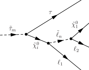
Figure 1: Schematic picture of stau decay.

The paper is organized as follows. In Section II we review stau mixing and the stau-neutralino Lagrangian with complex couplings. We calculate the amplitude squared for the entire stau decay in the spin-density matrix formalism Haber:1994pe . We construct the CP asymmetry from the normal tau polarization, and discuss its MSSM parameter dependence, as well its boost dependence for colliders like the ILC and LHC. In Section III, we numerically study the phase and parameter dependence of the asymmetry, and the stau and neutralino branching ratios. We comment on the impact of the ${\tilde{\tau}}_{2}$ decay in scenarios with nearly degenerate stau masses. We summarize and conclude in Section IV. The Appendices contain the definitions of momenta and spin vectors, the analytical expressions for the stau decay amplitudes in the spin-density matrix formalism, and formulae for the stau decay widths.

II Formalism

II.1 Stau mixing

In the complex MSSM, the stau mixing matrix in the $(\tilde{\tau}_{L},\tilde{\tau}_{R})$-basis is Haber:1984rc ; Bartl:2002uy

$$\mathcal{M}_{\tilde{\tau}}=\left(\begin{array}[]{cc}m^{2}_{\tilde{\tau}_{L}}&e^{-i\phi_{\tilde{\tau}}}m_{\tau}|\Lambda_{\tilde{\tau}}|\\ \\ e^{i\phi_{\tilde{\tau}}}m_{\tau}|\Lambda_{\tilde{\tau}}|&m^{2}_{\tilde{\tau}_{R}}\\ \end{array}\right).$$ (6)

CP violation is parameterized by the physical phase

$$\phi_{\tilde{\tau}} = {\rm arg}[\Lambda_{\tilde{\tau}}],$$ (7)

$$\Lambda_{\tilde{\tau}} = A_{\tau}-\mu^{*}\cot{\beta},$$ (8)

with the complex trilinear scalar coupling parameter $A_{\tau}$, the complex higgisino mass parameter $\mu$, and $\tan\beta=v_{1}/v_{2}$, the ratio of the vacuum expectation values of the two neutral Higgs fields. The left and right stau masses are

$$m^{2}_{\tilde{\tau}_{L}} = M^{2}_{{\tilde{L}}_{\tau}}+(-\frac{1}{2}+\sin^{2}\theta_{w})m^{2}_{Z}\cos(2\beta)+m^{2}_{\tau},$$ (9)

$$m^{2}_{\tilde{\tau}_{R}} = M^{2}_{{\tilde{E}}_{\tau}}-\sin^{2}\theta_{w}m^{2}_{Z}\cos(2\beta)+m^{2}_{\tau},$$ (10)

with the real soft SUSY breaking parameters $M^{2}_{{\tilde{L}_{\tau}},{\tilde{E}}_{\tau}}$, the electroweak mixing angle $\theta_{w}$, and the masses of the $Z$ boson $m_{Z}$, and of the tau lepton, $m_{\tau}$.

In the mass basis, the stop eigenstates are Haber:1984rc ; Bartl:2002uy

$$\left(\begin{array}[]{c}\tilde{\tau}_{1}\\ \tilde{\tau}_{2}\end{array}\right)=\mathcal{R}^{\tilde{\tau}}\left(\begin{array}[]{c}\tilde{\tau}_{L}\\ \tilde{\tau}_{R}\end{array}\right),$$ (11)

with the diagonalization matrix

$$\mathcal{R}^{\tilde{\tau}}=\left(\begin{array}[]{cc}e^{i\phi_{\tilde{\tau}}}\cos\theta_{\tilde{\tau}}&\sin\theta_{\tilde{\tau}}\\ -\sin\theta_{\tilde{\tau}}&e^{-i\phi_{\tilde{\tau}}}\cos\theta_{\tilde{\tau}}\end{array}\right),$$ (12)

and the stau mixing angle

$$\cos\theta_{\tilde{\tau}} = \frac{\displaystyle-m_{\tau}|\Lambda_{\tilde{\tau}}|}{\displaystyle\sqrt{m_{\tau}^{2}|\Lambda_{\tilde{\tau}}^{2}|+\left(m_{\tilde{\tau}_{1}}^{2}-m_{\tilde{\tau}_{2}}^{2}\right)^{2}}},$$ (13)

$$\sin\theta_{\tilde{\tau}} = \frac{\displaystyle m_{\tilde{\tau}_{L}}^{2}-m_{\tilde{\tau}_{1}}^{2}}{\displaystyle\sqrt{m_{\tau}^{2}|\Lambda_{\tilde{\tau}}^{2}|+\left(m_{\tilde{\tau}_{1}}^{2}-m_{\tilde{\tau}_{2}}^{2}\right)^{2}}}.$$ (14)

The stau mass eigenvalues are

$$m^{2}_{\tilde{\tau}_{1,2}} = \frac{1}{2}\bigg{[}\left(m_{\tilde{\tau}_{L}}^{2}+m_{\tilde{\tau}_{R}}^{2}\right)\mp$$ (15)

$$\phantom{\frac{1}{2}}\sqrt{\left(m_{\tilde{\tau}_{L}}^{2}-m_{\tilde{\tau}_{R}}^{2}\right)^{2}+4m_{\tilde{\tau}}^{2}|\Lambda_{\tilde{\tau}}|^{2}}~{}\bigg{]}.$$

II.2 Lagrangian and complex couplings

The relevant Lagrangian terms for the stau decay $\tilde{\tau}_{m}\to\tau\tilde{\chi}_{i}^{0}$ are Haber:1984rc ; Bartl:2002uy

$${\mathscr{L}}_{\tau\tilde{\tau}\tilde{\chi}^{0}}=g\,\bar{\tau}\,(a_{mi}^{\tilde{\tau}}\,P_{R}+b_{mi}^{\tilde{\tau}}\,P_{L})\,\tilde{\chi}_{i}^{0}\,\tilde{\tau}_{m}+{\rm h.c.},$$ (16)

with $P_{L,R}=(1\mp\gamma_{5})/2$, and the weak coupling constant $g=e/\sin\theta_{w}$, $e>0$. The couplings are defined as Bartl:2002uy

$$a_{mi}^{\tilde{\tau}}\equiv\sum^{2}_{n=1}\,(\mathcal{R}^{\tilde{\tau}}_{mn})^{\ast}\,{\cal A}_{in}^{\tau},\quad b_{mi}^{\tilde{\tau}}\equiv\sum^{2}_{n=1}\,(\mathcal{R}^{\tilde{\tau}}_{mn})^{\ast}\,{\cal B}_{in}^{\tau}.$$ (17)

The stau diagonalization matrix $\mathcal{R}^{\tilde{t}}$ is given in Eq. (2), and

$${\cal A}_{i}^{\tau}\equiv\left(\begin{array}[]{ccc}f_{\tau i}^{L}\\[5.69054pt] h_{\tau i}^{R}\end{array}\right),\qquad{\cal B}_{i}^{\tau}\equiv\left(\begin{array}[]{ccc}h_{\tau i}^{L}\\[5.69054pt] f_{\tau i}^{R}\end{array}\right).$$ (18)

In the photino, zino, higgsino basis ($\tilde{\gamma},\tilde{Z},\tilde{H}^{0}_{a},\tilde{H}^{0}_{b}$), we have

$$f_{\tau i}^{L} = \sqrt{2}\bigg{[}\frac{1}{\cos\theta_{w}}\left(\frac{1}{2}-\sin^{2}\theta_{w}\right)N_{i2}+\sin\theta_{w}N_{i1}\bigg{]},\qquad$$ (19)

$$f_{\tau i}^{R} = \sqrt{2}\sin\theta_{w}\left(\tan\theta_{w}N_{i2}^{*}-N_{i1}^{*}\right),$$ (20)

$$h_{\tau i}^{L} = (h_{\tau i}^{R})^{\ast}=-Y_{\tau}(N_{i3}^{\ast}\cos\beta+N_{i4}^{\ast}\sin\beta),$$ (21)

$$Y_{\tau} = \frac{m_{\tau}}{\sqrt{2}\,m_{W}\cos\beta},$$ (22)

with $m_{W}$ the mass of the $W$ boson, and $N$ the complex, unitary $4\times 4$ matrix that diagonalizes the neutralino mass matrix Haber:1984rc

$$N^{*}\cdot{\mathcal{M}}_{\tilde{\chi}^{0}}\cdot N^{\dagger}={\rm diag}(m_{\tilde{\chi}^{0}_{1}},\dots,m_{\tilde{\chi}^{0}_{4}}).$$ (23)

The interaction Lagrangian relevant for the neutralino decay $\tilde{\chi}_{i}^{0}\to\tilde{\ell}_{R,L}^{\pm}\ell^{\mp}$, for $\ell=e,\mu$ is Haber:1984rc

$${\mathscr{L}}_{\ell\tilde{\ell}\tilde{\chi}^{0}} = g\bar{\ell}f_{\ell i}^{L}P_{R}\tilde{\chi}_{i}^{0}\tilde{\ell}_{L}+g\bar{\ell}f_{\ell i}^{R}P_{L}\tilde{\chi}_{i}^{0}\tilde{\ell}_{R}+\mbox{h.c.},$$ (24)

with the couplings $f_{\ell i}^{L,R}$ given in Eqs. (19) and (20).

II.3 Tau spin density matrix

The unnormalized, $2\times 2$, hermitian, $\tau$ spin density matrix for stau decay, Eqs. (1) and (2), reads

$$\rho^{\lambda_{\tau}\lambda^{\prime}_{\tau}}\equiv\int\left(|\mathcal{M}|^{2}\right)^{\lambda_{\tau}\lambda^{\prime}_{\tau}}{{\rm d}\mathscr{L}\!\textsl{ips}},$$ (25)

with the amplitude $\mathcal{M}$, and the Lorentz invariant phase space element ${{\rm d}\mathscr{L}\!\textsl{ips}}$, for details see Appendix B. The $\tau$ helicities are denoted by $\lambda_{\tau}$ and $\lambda^{\prime}_{\tau}$. In the spin density matrix formalism Haber:1994pe , the amplitude squared is given by

$$\left(|\mathcal{M}|^{2}\right)^{\lambda_{\tau}\lambda^{\prime}_{\tau}}=|\Delta(\tilde{\chi}^{0}_{i})|^{2}|\Delta(\tilde{\ell})|^{2}\times$$ (26)

$$\sum_{\lambda_{i}\lambda_{i}^{\prime}}\rho_{D}(\tilde{\tau})^{\lambda_{\tau}\lambda_{\tau}^{\prime}}_{\lambda_{i}\lambda_{i}^{\prime}}\;\rho_{D_{1}}(\tilde{\chi}^{0}_{i})^{\lambda_{i}^{\prime}\lambda_{i}}\;D_{2}(\tilde{\ell}),$$

with the neutralino helicities $\lambda_{i},\,\lambda_{i}^{\prime}$. The amplitude squared decomposes into the remnants of the propagators

$$\Delta(j)=\dfrac{i}{s_{j}-m_{j}^{2}+im_{j}\Gamma_{j}},$$ (27)

with mass $m_{j}$, and width $\Gamma_{j}$ of particle $j=\tilde{\chi}^{0}_{i}$ or $\tilde{\ell}$, and the unnormalized spin density matrices for stau decay $\rho_{D}(\tilde{\tau})$, and neutralino decay $\rho_{D_{1}}(\tilde{\chi}^{0}_{i})$. The decay matrix of the spinless slepton is a factor since the polarizations of the final lepton and LSP are not accessible. The corresponding amplitude is denoted by $D_{2}(\tilde{\ell})$. Defining a set of spin basis vectors $s_{\tau}^{a}$ for the tau, see Eqs. (60) in Appendix A, and $s_{\tilde{\chi}^{0}_{i}}^{b}$ for the neutralino Kittel:2004rp , the spin density matrices can be expanded in terms of the Pauli matrices $\sigma$

$$\rho_{\rm D}(\tilde{\tau})^{\lambda_{\tau}\lambda_{\tau}^{\prime}}_{\lambda_{i}\lambda_{i}^{\prime}}={\rm D}\,\delta^{\lambda_{\tau}\lambda_{\tau}^{\prime}}\delta_{\lambda_{i}\lambda_{i}^{\prime}}+\Sigma_{\rm D}^{a}\,(\sigma^{a})^{\lambda_{\tau}\lambda_{\tau}^{\prime}}\delta_{\lambda_{i}\lambda_{i}^{\prime}}+$$

$$\Sigma_{\rm D}^{b}\,\delta^{\lambda_{\tau}\lambda_{\tau}^{\prime}}(\sigma^{b})_{\lambda_{i}\lambda_{i}^{\prime}}+\Sigma_{\rm D}^{ab}\,(\sigma^{a})^{\lambda_{\tau}\lambda_{\tau}^{\prime}}(\sigma^{b})_{\lambda_{i}\lambda_{i}^{\prime}},$$ (28)

$$\rho_{{\rm D}_{1}}({\tilde{\chi}}_{i}^{0})^{\lambda_{i}^{\prime}\lambda_{i}}={\rm D}_{1}\,\delta^{\lambda_{i}^{\prime}\lambda_{i}}+\Sigma_{{\rm D}_{1}}^{b}\,(\sigma^{b})^{\lambda_{i}^{\prime}\lambda_{i}},\phantom{spacespace}$$ (29)

with an implicit sum over $a,b=1,2,3$, respectively. The real expansion coefficients ${\rm D}$, ${\rm D_{1}}$, $\Sigma_{\rm D}^{a}$, $\Sigma_{\rm D}^{b}$, $\Sigma_{{\rm D}_{1}}^{b}$ and $\Sigma_{\rm D}^{ab}$ contain the physical information of the process. ${\rm D}$ denotes the unpolarized part of the amplitude for stau decay ${\tilde{\tau}}_{m}\to\chi^{0}_{i}\tau$ , ${\rm D_{1}}$ denotes the unpolarized part for neutralino decay $\chi^{0}_{i}\to{\tilde{\ell}}_{R}\ell_{1}$ , respectively. $\Sigma_{\rm D}^{a}$ gives the tau polarization, $\Sigma_{\rm D}^{b}$, and $\Sigma_{{\rm D}_{1}}^{b}$ describe the contributions from the neutralino polarization, and $\Sigma_{\rm D}^{ab}$ is the spin-spin correlation term, which contains the CP-sensitive parts. We give the expansion coefficients explicitly in Appendix C.

Inserting the density matrices, Eqs. (28) and (29), into Eq. (26), we get for the amplitude squared

$$(|\mathcal{M}|^{2})^{\lambda_{\tau}\lambda_{\tau}^{\prime}} = 2|\Delta({\tilde{\chi}^{0}}_{i})|^{2}|\Delta(\tilde{\ell})|^{2}\times$$ (30)

$$\Big{[}~{}({\rm D}{\rm D}_{1}+\Sigma_{\rm D}^{b}\Sigma_{{\rm D}_{1}}^{b})\delta^{\lambda_{\tau}\lambda_{\tau}^{\prime}}$$

$$+(\Sigma_{\rm D}^{a}{\rm D}_{1}+\Sigma_{\rm D}^{ab}\Sigma_{{\rm D}_{1}}^{b})(\sigma^{a})^{\lambda_{\tau}\lambda_{\tau}^{\prime}}\Big{]}{\rm D}_{2},\quad$$

with an implicit sum over $a,b=1,2,3$. The amplitude squared $(|\mathcal{M}|^{2})^{\lambda_{\tau}\lambda_{\tau}^{\prime}}$ is now decomposed into an unpolarized part (first summand), and into the part for the tau polarization (second summand), in Eq. (30). By using the completeness relations for the neutralino spin vectors, Eq. (62), the products in Eq. (30) can be written,

$$\Sigma^{b}_{\rm D}~{}\Sigma^{b}_{{\rm D}_{1}} = \,{}^{\;\,+}_{(-)}\frac{g^{4}}{2}\left(|a^{\tilde{\tau}}_{mi}|^{2}-|b^{\tilde{\tau}}_{mi}|^{2}\right)|f^{R}_{\ell i}|^{2}\times$$ (31)

$$\left[m_{\tilde{\chi}_{i}^{0}}^{2}(p_{\tau}\cdot p_{\ell_{1}})-(p_{\tilde{\chi}_{i}^{0}}\cdot p_{\tau})(p_{\ell_{1}}\cdot p_{\tilde{\chi}_{i}^{0}})\right],\quad$$

$$\Sigma^{ab}_{\rm D}~{}\Sigma^{b}_{{\rm D}_{1}} = \,{}^{\;\,+}_{(-)}\frac{g^{4}}{2}\left(|a^{\tilde{\tau}}_{mi}|^{2}+|b^{\tilde{\tau}}_{mi}|^{2}\right)|f^{R}_{\ell i}|^{2}m_{\tau}\times$$ (32)

$$\left[(s^{a}_{\tau}\cdot p_{\tilde{\chi}_{i}^{0}})(p_{\tilde{\chi}_{i}^{0}}\cdot p_{\ell_{1}})-m_{\tilde{\chi}_{i}^{0}}^{2}(s^{a}_{\tau}\cdot p_{\ell_{1}})\right]$$

$$\,{}^{\;\,+}_{(-)}g^{4}\mathfrak{Re}\{a^{\tilde{\tau}}_{mi}(b^{\tilde{\tau}}_{mi})^{\ast}\}|f^{R}_{\ell i}|^{2}m_{\tilde{\chi}_{i}^{0}}\times$$

$$\left[(p_{\tau}\cdot p_{\tilde{\chi}_{i}^{0}})(s^{a}_{\tau}\cdot p_{\ell_{1}})-(p_{\tau}\cdot p_{\ell_{1}})(s^{a}_{\tau}\cdot p_{\tilde{\chi}_{i}^{0}})\right]$$

$$\,{}^{\;\,+}_{(-)}g^{4}|f^{R}_{\ell i}|^{2}m_{\tilde{\chi}_{i}^{0}}\times$$

$$\mathfrak{Im}\{a^{\tilde{\tau}}_{mi}(b^{\tilde{\tau}}_{mi})^{\ast}\}[p_{\tilde{\tau}},~{}p_{\ell_{1}},~{}p_{\tau},~{}s^{a}_{\tau}].$$

The spin-spin correlation term $\Sigma^{ab}_{\rm D}~{}\Sigma^{b}_{{\rm D}_{1}}$, Eq. (32), explicitly depends on the imaginary part $\mathfrak{Im}\{a^{\tilde{\tau}}_{mi}(b^{\tilde{\tau}}_{mi})^{\ast}\}$ of the stau-tau-neutralino couplings, Eq. (16). Thus this term is manifestly CP-sensitive, i.e., it depends on the phases $\phi_{A_{\tau}}$, $\phi_{1}$, $\phi_{\mu}$ of the stau-tau-neutralino sector. The imaginary part is multiplied by the totally anti-symmetric (epsilon) product,

$$\mathcal{E}^{a}\equiv[p_{\tilde{\tau}},~{}p_{\ell_{1}},~{}p_{\tau},~{}s^{a}_{\tau}]\equiv\epsilon_{\mu\nu\rho\sigma}\,p_{\tilde{\tau}}^{\mu}\,p_{\ell_{1}}^{\nu}\,p_{\tau}^{\rho}\,s^{a,\sigma}_{\tau},$$ (33)

with the convention $\epsilon_{0123}=1$. Since each of the spatial components of the four-momenta $p$, or the spin vectors $s^{a}_{\tau}$, changes sign under a time transformation, $t\to-t$, the epsilon product $\mathcal{E}^{a}$ is T-odd. In the stau rest frame, $p_{\tilde{\tau}}^{\mu}=(m_{\tilde{\tau}},\mathbf{0})$, the epsilon product reduces to the T-odd triple product ${\mathcal{T}}^{a}$

$$[p_{\tilde{\tau}},~{}p_{\ell_{1}},~{}p_{\tau},~{}s^{a}_{\tau}]=m_{\tilde{\tau}}\;\,(\mathbf{p}_{\ell_{1}}\times\mathbf{p}_{\tau})\cdot\mathbf{s}^{a}_{\tau}\equiv m_{\tilde{\tau}}\,{\mathcal{T}}^{a}.$$ (34)

The task in the next section is to define an observable that projects out from the amplitude squared the part proportional to $\mathcal{E}^{a}$ (or ${\mathcal{T}}^{a}$), in order to probe the CP-sensitive coupling combination $\mathfrak{Im}\{a^{\tilde{\tau}}_{mi}(b^{\tilde{\tau}}_{mi})^{\ast}\}$.

II.4 Normal tau polarization and CP asymmetry

The $\tau$ polarization is given by the expectation value of the Pauli matrices $\sigma$$=(\sigma_{1},\sigma_{2},\sigma_{3})$ Renard:1981de

$$\mbox{\boldmath$\mathcal{P}$ }=\frac{{\rm Tr}\{\rho\mbox{\boldmath$\sigma$}\}}{{\rm Tr}\{\rho\}},$$ (35)

with the $\tau$ spin density matrix $\rho$, as given in Eq. (25). In our convention for the polarization vector $\mathcal{P}$ $=(\mathcal{P}_{1},\mathcal{P}_{2},\mathcal{P}_{3})$, the components $\mathcal{P}_{1}$ and $\mathcal{P}_{3}$ are the transverse and longitudinal polarizations in the plane spanned by ${\bf p}_{\ell_{1}}$ and ${\bf p}_{\tau}$, respectively, and $\mathcal{P}_{2}$ is the polarization normal to that plane. See our definition of the tau spin basis vectors $s_{\tau}^{a}$ in Appendix A.

The normal $\tau$ polarization is equivalently defined as

$$\mathcal{P}_{2} \equiv \frac{N(\uparrow)-N(\downarrow)}{N(\uparrow)+N(\downarrow)},$$ (36)

with the number of events $N$ with the $\tau$ spin up $(\uparrow)$ or down $(\downarrow)$, with respect to the quantization axis ${\bf p}_{\ell_{1}}\times{\bf p}_{\tau}$, see Eq. (60). The normal $\tau$ polarization can thus also be regarded as an asymmetry

$$\mathcal{P}_{2}=\frac{\sigma(\mathcal{T}>0)-\sigma(\mathcal{T}<0)}{\sigma(\mathcal{T}>0)+\sigma(\mathcal{T}<0)},$$ (37)

of the triple product

$$\mathcal{T}=({\bf p}_{\ell_{1}}\times{\bf p}_{\tau})\cdot{\mbox{\boldmath$\xi$}}_{\tau},$$ (38)

where $\xi$_τ is the direction of the $\tau$ spin vector for each event. The triple product $\mathcal{T}$ is included in the spin-spin correlation term $\Sigma^{ab}_{\rm D}~{}\Sigma^{b}_{{\rm D}_{1}}$, Eq. (32), cf. Eq. (34), and the asymmetry thus probes the term which contains the CP-sensitive coupling combination $\mathfrak{Im}\{a^{\tilde{\tau}}_{mi}(b^{\tilde{\tau}}_{mi})^{\ast}\}$.

Since under naive time reversal, $t\to-t$, the triple product $\mathcal{T}$ changes sign, the tau polarization $\mathcal{P}_{2}$, Eq. (37), is T-odd. Due to CPT invariance Luders:1954zz , $\mathcal{P}_{2}$ would thus be CP-odd at tree level. In general, $\mathcal{P}_{2}$ also has contributions from absorptive phases, e.g. from intermediate $s$-state resonances or final-state interactions, which do not signal CP violation. Although such absorptive contributions are a higher order effect, and thus expected to be small, they can be eliminated in the true CP asymmetry Bartl:2003gr

$${\mathcal{A}_{\tau}^{\rm CP}}=\frac{1}{2}(\mathcal{P}_{2}-\bar{\mathcal{P}}_{2}),$$ (39)

where $\bar{\mathcal{P}}_{2}$ is the normal tau polarization for the charged conjugated process $\tilde{\tau}_{m}^{\ast}\to\tau^{+}\tilde{\chi}_{i}^{0}$. For our analysis at tree level, where no absorptive phases are present, we find $\bar{\mathcal{P}}_{2}=-\mathcal{P}_{2}$, see the sign change in Eqs. (31) and (32), and thus ${\mathcal{A}_{\tau}^{\rm CP}}=\mathcal{P}_{2}$. We study ${\mathcal{A}_{\tau}^{\rm CP}}$ in the following, which is, however, equivalent to $\mathcal{P}_{2}$ at tree level.

Inserting now the explicit form of the density matrix $\rho$, Eq. (25), into Eq. (35), together with Eq. (30), we obtain the CP asymmetry

$${\mathcal{A}_{\tau}^{\rm CP}}=\mathcal{P}_{2}=\frac{\int\Sigma^{a=2,b}_{\rm D}~{}\Sigma^{b}_{{\rm D}_{1}}\,{{\rm d}\mathscr{L}\!\textsl{ips}}}{\int{\rm D}{\rm D}_{1}\,{{\rm d}\mathscr{L}\!\textsl{ips}}},$$ (40)

where we have used the narrow width approximation for the propagators in the phase space element ${{\rm d}\mathscr{L}\!\textsl{ips}}$, see Eq. (87). Note that in the denominator of ${\mathcal{A}_{\tau}^{\rm CP}}$, Eq. (40), the spin correlation terms vanish, $\int\Sigma^{b}_{\rm D}~{}\Sigma^{b}_{{\rm D}_{1}}\,{{\rm d}\mathscr{L}\!\textsl{ips}}=0$, see Eq. (31), when integrated over phase space. In the numerator only the spin-spin correlation term $\Sigma^{ab}_{\rm D}~{}\Sigma^{b}_{{\rm D}_{1}}$ for $a=2$ contributes, which contains the T-odd epsilon product $\mathcal{E}^{a}$, see Eq. (33).

II.5 Parameter dependence of the CP asymmetry

To qualitatively understand the dependence of the asymmetry ${\mathcal{A}_{\tau}^{\rm CP}}$, Eq. (40), on the MSSM parameters, we study in some detail its dependence on the $\tilde{\tau}_{m}$-$\tau$-$\tilde{\chi}_{i}^{0}$ couplings, $a^{\tilde{\tau}}_{mi}$ and $b^{\tilde{\tau}}_{mi}$, see Eq. (81). From the explicit form of the decay terms $\Sigma^{b}_{\rm D}~{}\Sigma^{b}_{{\rm D}_{1}}$ Eq. (31), and ${\rm D}$, ${\rm D}_{1}$, Eqs. (69), (73), respectively, we find that the asymmetry

$${\mathcal{A}_{\tau}^{\rm CP}} = \eta_{mi}\;\frac{m_{{\tilde{\chi}^{0}}_{i}}\int[p_{\tilde{\tau}},~{}p_{\ell_{1}},~{}p_{\tau},~{}s^{a=2}_{\tau}]\,{\rm d}\mathscr{L}\!\textsl{ips}}{(p_{{\tilde{\chi}}_{i}^{0}}\cdot p_{\tau})(p_{{\tilde{\chi}}_{i}^{0}}\cdot p_{\ell_{1}})\,\int{\rm d}\mathscr{L}\!\textsl{ips}},$$ (41)

with $(p_{{\tilde{\chi}}_{i}^{0}}\cdot p_{\tau})=(m_{\tilde{\tau}}^{2}-m_{\tilde{\chi}_{i}^{0}}^{2})/2$, and $(p_{\tilde{\chi}^{0}_{i}}\cdot p_{\ell_{1}})=(m_{\tilde{\chi}_{i}^{0}}^{2}-m_{\tilde{\ell}}^{2})/2$, is proportional to the decay coupling factor

$$\eta_{mi}=\frac{\mathfrak{Im}\{a^{\tilde{\tau}}_{mi}(b^{\tilde{\tau}}_{mi})^{\ast}\}}{\frac{1}{2}(|a^{\tilde{\tau}}_{mi}|^{2}+|b^{\tilde{\tau}}_{mi}|^{2})},$$ (42)

with $\eta_{mi}\in[-1,1]$. We thus expect maximal asymmetries for equal moduli of left and right couplings, $|a^{\tilde{\tau}}_{mi}|\approx|b^{\tilde{\tau}}_{mi}|$, which have a phase difference of about $\pi/2$, where the coupling factor can be maximal $\eta_{mi}=\pm 1$, see Eq. (42).

To study the dependence of $\eta$ on the CP phase $\phi_{\tilde{\tau}}$ of the stau sector, and the stau mixing angle $\theta_{\tilde{\tau}}$, we expand the imaginary part of the product of $\tilde{\tau}_{m}$-$\tau$-$\tilde{\chi}_{i}^{0}$ couplings

$$\mathfrak{Im}\{a^{\tilde{\tau}}_{mi}(b^{\tilde{\tau}}_{mi})^{\ast}\} = \mathfrak{Im}\Big{\{}|\mathcal{R}_{m1}|^{2}f^{L}_{\tau i}h^{R}_{\tau i}+|\mathcal{R}_{m2}|^{2}f^{\ast R}_{\tau i}h^{R}_{\tau i}$$ (43)

$$+ \mathcal{R}_{m1}\mathcal{R}_{m2}^{\ast}\big{[}(h^{R}_{\tau i})^{2}-f^{R}_{\tau i}f^{\ast L}_{\tau i}\big{]}\Big{\}},$$

in terms of the stau mixing matrix $\mathcal{R}$, the gauge couplings $f_{\tau i}^{L,R}$ and the higgs couplings $h_{\tau i}^{L,R}$. In particular, for a CP-conserving neutralino sector, $\phi_{1}=\phi_{\mu}=0$, we have

$$\mathfrak{Im}\{a^{\tilde{\tau}}_{mi}(b^{\tilde{\tau}}_{mi})^{\ast}\}=\,^{\;\,+}_{(-)}\sin\phi_{\tilde{\tau}}\sin(2\theta_{\tilde{\tau}})\frac{1}{2}\left[(h^{R}_{\tau i})^{2}-f^{R}_{\tau i}f^{L}_{\tau i}\right],$$

(44)

for $m=1$, and the sign in parentheses holds for $m=2$. Thus we expect a maximal $\eta$ and thus maximal asymmetries for maximal stau mixing, $\theta_{\tilde{\tau}}\approx\pm\pi/4$, and a maximal CP phase in the stau mixing matrix, $\phi_{\tilde{\tau}}\approx\pm\pi/2$. Note that, in particular, the dependence of $\phi_{\tilde{\tau}}$ on $\phi_{A_{\tau}}$ is strong for $|A_{\tau}|>|\mu|\tan\beta$. We will study numerically the phase and parameter dependence on ${\mathcal{A}_{\tau}^{\rm CP}}$ and $\eta$ further in Section III.

II.6 Boost dependence

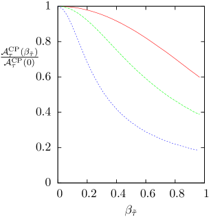
Figure 2: Boost distributions of the $\tau$ polarization asymmetry ${\mathcal{A}_{\tau}^{\rm CP}}$, Eq. (39), normalized by ${\mathcal{A}_{\tau}^{\rm CP}}(\beta_{\tilde{\tau}}=0)$, for three different sets of stau masses, $m_{\tilde{\tau}_{1,2}}\approx 200$ GeV (solid, red), $400$ GeV (dashed, green), and $1000$ TeV (dotted, blue), see text, for stau decay $\tilde{\tau}_{1}\to\tau\tilde{\chi}_{2}^{0}$, followed by $\tilde{\chi}_{2}^{0}\to\ell_{1}\tilde{\ell}_{R}$, and $\tilde{\ell}_{R}\to\tilde{\chi}^{0}_{1}\ell_{2}$ ($\ell=e$ or $\mu$), see Fig. 1, The SUSY parameters are given in Table 1.

The triple product asymmetry ${\mathcal{A}_{\tau}^{\rm CP}}$, Eq. (40), is not Lorentz invariant but depends on the boost of the decaying stau,

$$\beta_{\tilde{\tau}}=\dfrac{|{\bf p}_{\tilde{\tau}}|}{E_{\tilde{\tau}}}.$$ (45)

In Fig. 2, we show the boost dependence of the asymmetry ${\mathcal{A}_{\tau}^{\rm CP}}(\beta_{\tilde{\tau}})$, normalized by ${\mathcal{A}_{\tau}^{\rm CP}}(\beta_{\tilde{\tau}}=0)$. The SUSY parameters are given in Table 1, and we have chosen three sets of different $\tilde{\tau}$ soft-breaking parameters $\{M_{{\tilde{E}}_{\tau}},M_{{\tilde{L}}_{\tau}}\}=\{195,200\}$ GeV (solid, red); $\{395,400\}$ GeV (dashed, green); and $\{998,1000\}$ GeV (dotted, blue). The corresponding stau masses are $\{m_{\tilde{\tau}_{1}},m_{\tilde{\tau}_{2}}\}=\{194,209\}$; $\{395,404\}$; $\{998,1002\}$ GeV, respectively. The corresponding asymmetries in the stau rest frame are ${\mathcal{A}_{\tau}^{\rm CP}}(\beta_{\tilde{\tau}})=-66\%$; $-72\%$, $-71\%$. Note that we have chosen nearly degenerate stau masses which lead to an enhanced stau mixing and thus to maximal asymmetries; see also the discussion in Section III.

For the stau masses $\{m_{\tilde{\tau}_{1}},m_{\tilde{\tau}_{2}}\}=\{194,209\}$ GeV, the staus can be produced at the ILC with $\sqrt{s}=500$ GeV, and have a fixed boost of $\beta_{\tilde{\tau}}=0.63$. The corresponding asymmetry is then reduced to ${\mathcal{A}_{\tau}^{\rm CP}}=-53\%$ if the stau rest frame cannot be reconstructed. Typical ILC cross section for these masses are of the order of some $20$ fb Alwall:2007st .

If the staus are produced at the LHC, they will have a distinct boost distribution depending on their mass, which typically peaks at high values $\beta_{\tilde{\tau}}\approx 0.9$ for stau masses of the order of a few $100$ GeV up to a $1$ TeV, see e.g. Refs Deppisch:2009nj ; Deppisch:2010nc . Then the normal tau polarization in the laboratory frame is obtained by folding the boost dependent polarization ${\mathcal{A}_{\tau}^{\rm CP}}$ with the normalized stau boost distribution Deppisch:2009nj ,

$${\mathcal{A}_{\tau}^{\rm CP}}_{\rm lab}=\dfrac{1}{\sigma_{P}}\int_{0}^{1}\dfrac{{\rm d}\sigma_{P}}{{\rm d}\beta_{\tilde{\tau}}}{\mathcal{A}_{\tau}^{\rm CP}}(\beta_{\tilde{\tau}})\,{\rm d}\beta_{\tilde{\tau}},$$ (46)

with the production cross section $\sigma_{P}=\sigma(pp\to\tilde{\tau}^{+}\tilde{\tau}^{-})$. The typical reduction of the normal tau polarization ${\mathcal{A}_{\tau}^{\rm CP}}_{\rm lab}$ is of the order of two thirds of the asymmetry compared to that in the stau rest frame ${\mathcal{A}_{\tau}^{\rm CP}}(0)$. However, it has been recently shown (for similar asymmetries in stop decays at the LHC), that the rest frame can be partly reconstructed event by event using on-shell mass conditions, see Refs. MoortgatPick:2009jy . The LHC cross section for stau pair production, $\sigma(pp\to\tilde{\tau}_{1}^{+}\tilde{\tau}_{1}^{-})$, also sensitively depends on the stau masses, e.g., for our benchmark scenario in Table 1, we find cross sections up to $10$ fb at $\sqrt{s}=14$ TeV Alwall:2007st .

Table 1: Benchmark scenario. The mass parameters $M_{2}$, $|\mu|$, $A_{\tau}$, $M_{\tilde{E}}$, $M_{\tilde{L}}$ $M_{{\tilde{E}}_{\tau}}$, and $M_{{\tilde{L}}_{\tau}}$ are given in GeV.

${{\phi_{1}}_{\phantom{I}}}_{\phantom{I}}$		${{\phi_{\mu}}_{\phantom{I}}}_{\phantom{I}}$		${{\phi_{A_{\tau}}}_{\phantom{I}}}_{\phantom{I}}$		${M_{2}}_{\phantom{I}}$		${|\mu|}_{\phantom{I}}$		${A_{\tau}}_{\phantom{I}}$		${\tan\beta}_{\phantom{I}}$
0		0		$\pi/2$		250		250		2000		3
${M_{{\tilde{E}}_{\tau}}}_{\phantom{I}}$				${M_{{\tilde{L}}_{\tau}}}_{\phantom{I}}$				${M_{\tilde{E}}}_{\phantom{I}}$				${M_{\tilde{L}}}_{\phantom{I}}$
495				500				150				200

Table 2: Mass spectrum for the scenario in Table 1.

${\tilde{\ell}}$		$m$ [GeV]								$\tilde{\chi}$		$m$ [GeV]
${\tilde{e}}_{R},{\tilde{\mu}}_{R}$		155								${\tilde{\chi}}_{1}^{0}$		112
${\tilde{e}}_{L},{\tilde{\mu}}_{L}$		204								${\tilde{\chi}}_{2}^{0}$		190
${\tilde{\nu}}_{e},{\tilde{\nu}}_{\mu}$		192								${\tilde{\chi}}_{3}^{0}$		254
${\tilde{\nu}}_{\tau}$		497								${\tilde{\chi}}_{4}^{0}$		327
${\tilde{\tau}}_{1}$		495								${\tilde{\chi}}_{1}^{\pm}$		181
${\tilde{\tau}}_{2}$		504								${\tilde{\chi}}_{2}^{\pm}$		325

III Numerical results

We quantitatively study the tau polarization asymmetry, and the branching ratios for the two-body decay chain

$$\tilde{\tau}_{1}\to\tau+\tilde{\chi}_{2}^{0};\quad\tilde{\chi}_{2}^{0}\to\ell_{1}^{+}+\tilde{\ell}_{R}^{-};\quad\tilde{\ell}_{R}^{-}\to\tilde{\chi}^{0}_{1}+\ell_{2}^{-},$$ (47)

for $\ell=e,\mu$. The asymmetry probes the MSSM phases $\phi_{1}$, $\phi_{\mu}$ and $\phi_{A_{\tau}}$, of the neutralino and stau sector. We center our numerical discussion around a general MSSM benchmark scenario, see Table 1. We choose heavier soft breaking parameters in the stau sector than in the $\tilde{e},\tilde{\mu}$ sector, to enable the mass hierarchy

$$m_{\tilde{\tau}_{m}}>m_{\tilde{\chi}_{i}^{0}}>m_{\tilde{\ell}_{R}}>m_{\tilde{\chi}_{1}^{0}}.$$ (48)

Further we choose almost degenerate staus which enhances their mixing, leading to maximal asymmetries. We choose a large value of the trilinear scalar coupling parameter, $|A_{\tau}|>|\mu|\tan\beta$, to enhance the impact of $\phi_{A_{\tau}}$ in the stau sector. Finally, to reduce the number of MSSM parameters, we use the (GUT inspired) relation $|M_{1}|=5/3\,M_{2}\tan^{2}\theta_{w}$ Haber:1984rc for the gaugino mass parameters. The resulting masses of the staus, neutralinos and charginos are summarized in Table 2.

III.1 Phase dependence

For the benchmark scenario given in Table 1, we study the phase dependence of the asymmetry ${\mathcal{A}_{\tau}^{\rm CP}}$ in the stau rest frame. In Fig. 3, we show the dependence on the CP phases in the neutralino sector, $\phi_{1}$ and $\phi_{\mu}$. In Fig. 3, we show the dependence on the phases in the stau secotor $\phi_{A_{\tau}}$ and $\phi_{\mu}$. The asymmetry strongly depends on $\phi_{A_{\tau}}\approx\phi_{\tilde{\tau}}$, which we expect for $|A_{\tau}|\gg|\mu|\tan\beta$ as in our benchmark scenario, see Table 1. In particular for $\phi_{\mu}=0$ in Fig. 3, the asymmetry follows the approximation formula Eq. (44), and attains its maximal values at $\phi_{\tilde{\tau}}\approx\phi_{A_{\tau}}\approx\pm\pi/2$.

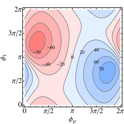
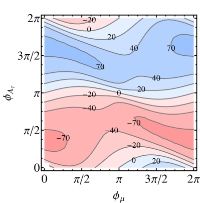
Figure 3: Phase dependence of (a) the $\tau$ polarization asymmetry ${\mathcal{A}_{\tau}^{\rm CP}}$, Eq. (39), in percent, in the $\phi_{1}$–$\phi_{\mu}$ plane (for $\phi_{A_{\tau}}=0$), and (b) in the $\phi_{A_{\tau}}$–$\phi_{\mu}$ plane (for $\phi_{1}=0$), in the stau rest frame. We consider the decay $\tilde{\tau}_{1}\to\tau\tilde{\chi}_{2}^{0}$, followed by $\tilde{\chi}_{2}^{0}\to\ell_{1}^{+}\tilde{\ell}_{R}^{-}$, and $\tilde{\ell}_{R}^{-}\to\tilde{\chi}^{0}_{1}\ell_{2}^{-}$ where $\ell=e$ or $\mu$, cf. Fig. 1. The other MSSM parameters are defined in Table 1.

III.2 $|A_{\tau}|$–$\tan\beta$ dependence and stau mixing

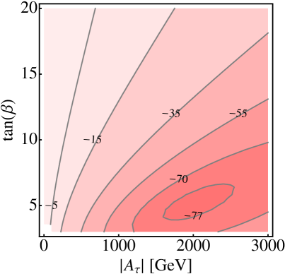
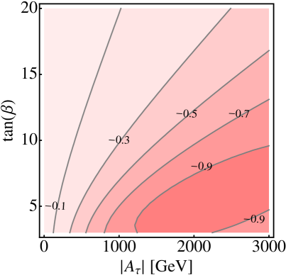
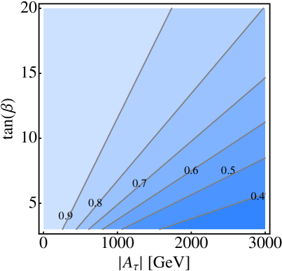
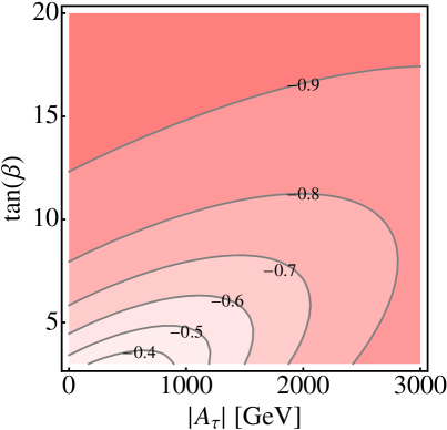
Figure 4: $|A_{\tau}|$–$\tan\beta$ dependence of (a) the $\tau$ polarization asymmetry ${\mathcal{A}_{\tau}^{\rm CP}}$, Eq. (39), in percent, in the stau rest frame (for the decay $\tilde{\tau}_{1}\to\tau\tilde{\chi}_{2}^{0}$, followed by $\tilde{\chi}_{2}^{0}\to\ell_{1}^{+}\tilde{\ell}_{R}^{-}$, and $\tilde{\ell}_{R}^{-}\to\tilde{\chi}^{0}_{1}\ell_{2}^{-}$ for $\ell=e$ or $\mu$, cf. Fig. 1), (b) the coupling factor $\eta$, Eq. (42), (c) the phase $\phi_{\tilde{\tau}}$ in the stau sector, Eq. (7), and (d) $\sin(2\theta_{\tilde{\tau}})$, with $\theta_{\tilde{\tau}}$ the stau mixing angle, Eqs. (13), (14). The plots are for $\phi_{A_{\tau}}=\pi/4,$ the other MSSM parameters are given in Table 1.

In Fig. 4, we show the $|A_{\tau}|$ and $\tan\beta$ dependence of the asymmetry ${\mathcal{A}_{\tau}^{\rm CP}}$ in the stau rest frame. We can observe that the asymmetry obtains its maximum, ${\mathcal{A}_{\tau}^{\rm CP}}\approx-77\%$, where also the coupling factor is maximal, $\eta\approx 0.95$, see Fig. 4. As discussed in Subsection II.5, the imaginary part of the product of the stau couplings $\mathfrak{Im}\{a^{\tilde{\tau}}_{mi}(b^{\tilde{\tau}}_{mi})^{\ast}\}$ is maximal for a maximal CP phase $\phi_{\tilde{\tau}}=\pi/2$ in the stau sector, which we show in Fig. 4. Note that the location of the maximum of ${\mathcal{A}_{\tau}^{\rm CP}}$ is not at maximal stau mixing, $\sin(\theta_{\tilde{\tau}})=1/\sqrt{2}\approx 0.7$, since $\eta\propto\sin(2\theta_{\tilde{\tau}})/(|a^{\tilde{\tau}}|^{2}+|b^{\tilde{\tau}}|^{2})$ starts to decrease for increasing $A_{\tau}$ and $\tan\beta$.

To study the stau mixing, we show the $M_{{\tilde{E}}_{\tau}}$–$M_{{\tilde{L}}_{\tau}}$ dependence of the asymmetry ${\mathcal{A}_{\tau}^{\rm CP}}$ in Fig. 5. In the entire $M_{{\tilde{E}}_{\tau}}$–$M_{{\tilde{L}}_{\tau}}$ plane, the CP phase in the stau sector is almost maximal, $\phi_{\tilde{\tau}}=0.61\pi$. However, the asymmetry obtains its maxima in the small corridor $M_{{\tilde{E}}_{\tau}}\approx M_{{\tilde{L}}_{\tau}}$, where the stau mixing is maximal, $\theta_{\tilde{\tau}}=\pi/4$.

III.3 $|\mu|$–$M_{2}$ dependence and branching ratios

We show the $|\mu|$–$M_{2}$ dependence of the asymmetry ${\mathcal{A}_{\tau}^{\rm CP}}$ in Fig. 5. The maxima of ${\mathcal{A}_{\tau}^{\rm CP}}$ are obtained where the coupling factor $\eta$ is also maximal, see Eq. (42).

In Fig. 6, we show the corresponding stau branching ratio, ${\rm BR}(\tilde{\tau}_{1}\to\tau\tilde{\chi}_{2}^{0})$, which can be as large as $40$%. Other competing channels can reach ${\rm BR}(\tilde{\tau}_{1}\to\tau\tilde{\chi}_{1}^{0})\approx 65\%$, and ${\rm BR}(\tilde{\tau}_{1}\to\nu_{\tau}\tilde{\chi}_{1(2)}^{\pm})\approx 20(10)\%$. The stau decay into the chargino $\tilde{\chi}_{1}^{\pm}$ is always open since typically the second lightest neutralino and the lightest chargino are almost degenerate, $m_{\tilde{\chi}_{2}^{0}}\approx m_{\tilde{\chi}_{1}^{\pm}}$. The neutralino branching ratio ${\rm BR}(\tilde{\chi}_{2}^{0}\to\ell\tilde{\ell}_{R})$, summed over $\ell=e,\mu$, is shown in Fig. 6, which reaches up to $100$%. The other important competing decay channels are ${\rm BR}(\tilde{\chi}_{2}^{0}\to\nu_{\ell}\tilde{\nu}_{\ell})$, and ${\rm BR}(\tilde{\chi}_{2}^{0}\to\ell\tilde{\ell}_{L})$, which open around $\mu\approx 250$ GeV and $\mu\approx 300$ GeV, respectively, for $M_{2}=250$ GeV. Note that in our benchmark scenario, see Table 1, we have ${\rm BR}(\tilde{\ell}_{R}\to\tilde{\chi}^{0}_{1}\ell)=1$.

III.4 Impact of $\tilde{\tau}_{2}$ decay

As we discussed in Section III.2, we find large asymmetries for nearly degenerate staus, where we naturally obtain a maximal stau mixing. However, then typically the asymmetries for $\tilde{\tau}_{1}$ and $\tilde{\tau}_{2}$ decay are similar in magnitude, but opposite in sign. For example in our benchmark scenario we find ${\mathcal{A}_{\tau}^{\rm CP}}=-71\%$ for $\tilde{\tau}_{1}$ decay, but ${\mathcal{A}_{\tau}^{\rm CP}}=+32\%$ for the decay of $\tilde{\tau}_{2}$. If the production and decay process of $\tilde{\tau}_{1}$ cannot be experimentally disentangled from that of $\tilde{\tau}_{2}$ properly, the two asymmetries might cancel. We show their sum in Fig. 7 in the $M_{{\tilde{E}}_{\tau}}$–$M_{{\tilde{L}}_{\tau}}$ plane. In Fig. 7, we show the corresponding stau mass splitting.

Note that also the stau branching ratios are similar in size; for example in our benchmark scenario we have ${\rm BR}(\tilde{\tau}_{1}\to\tau\tilde{\chi}_{2}^{0})=18\%$, and ${\rm BR}(\tilde{\tau}_{2}\to\tau\tilde{\chi}_{2}^{0})=30\%$. For the $M_{{\tilde{E}}_{\tau}}$–$M_{{\tilde{L}}_{\tau}}$ plane shown in Fig. 5, the decay branching ratio ${\rm BR}(\tilde{\tau}_{1}\to\tau\tilde{\chi}_{2}^{0})$ is at least $10\%$, and that of $\tilde{\tau}_{2}$ is larger by roughly a factor of $2$ to $4$.

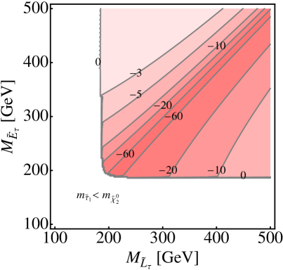
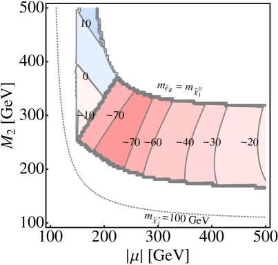
Figure 5: Dependence of the $\tau$ polarization asymmetry ${\mathcal{A}_{\tau}^{\rm CP}}$, Eq. (39), in percent, in the stau rest frame (for the decay $\tilde{\tau}_{1}\to\tau\tilde{\chi}_{2}^{0}$, followed by $\tilde{\chi}_{2}^{0}\to\ell_{1}^{+}\tilde{\ell}_{R}^{-}$, and $\tilde{\ell}_{R}^{-}\to\tilde{\chi}^{0}_{1}\ell_{2}^{-}$ for $\ell=e$ or $\mu$, see Fig. 1), on (a) the soft breaking parameters in the stau sector $M_{{\tilde{E}}_{\tau}}$, $M_{{\tilde{L}}_{\tau}}$, Eqs. (9), Eqs. (10). In (b) the dependence of ${\mathcal{A}_{\tau}^{\rm CP}}$ on the gaugino and higgsino parameters $|\mu|$, $M_{2}$. Below the contour $m_{\tilde{e}_{R}}=m_{\tilde{\chi}_{2}^{0}}$ the two-body decay $\tilde{\chi}_{2}^{0}\to\ell\tilde{\ell}_{R}$ is kinematically forbidden, above the contour $m_{\tilde{e}_{R}}=m_{\tilde{\chi}_{1}^{0}}$ the lightest neutralino is no longer the LSP since $m_{\tilde{e}_{R}}<m_{\tilde{\chi}_{1}^{0}}$. Below the contour $m_{\tilde{\chi}_{1}^{\pm}}=100$ GeV the lightest chargino is lighter than $100$ GeV. The MSSM parameters are given in Table 1.

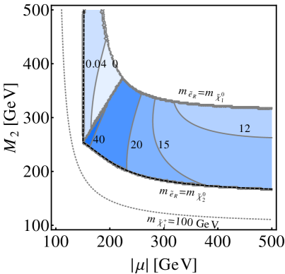
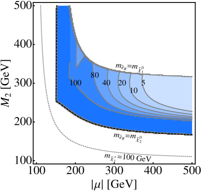
Figure 6: Contour lines in the $|\mu|$–$M_{2}$ plane of (a) the stau branching ratio ${\rm BR}(\tilde{\tau}_{1}\to\tau\tilde{\chi}_{2}^{0})$ in percent, and (b) the neutralino branching ratio ${\rm BR}(\tilde{\chi}_{2}^{0}\to\ell\tilde{\ell}_{R})$, in percent, summed over both lepton flavors $\ell=e$, $\mu$ and charges, for the MSSM parameters as given in Table 1. Below the contours $m_{\tilde{e}_{R}}=m_{\tilde{\chi}_{2}^{0}}$ in Figs. 6, 6, the two-body decay $\tilde{\chi}_{2}^{0}\to\ell\tilde{\ell}_{R}$ is kinematically forbidden, above the contours $m_{\tilde{e}_{R}}=m_{\tilde{\chi}_{1}^{0}}$ the lightest neutralino is no longer the LSP since $m_{\tilde{e}_{R}}<m_{\tilde{\chi}_{1}^{0}}$. Below the contours $m_{\tilde{\chi}_{1}^{\pm}}=100$ GeV the lightest chargino is lighter than $100$ GeV.

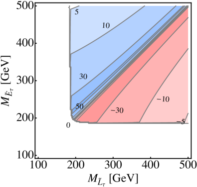
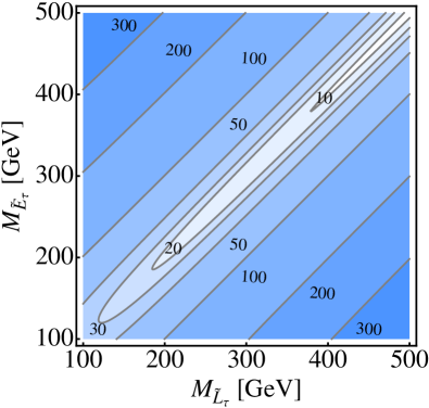
Figure 7: Contour lines of (a) the sum of the $\tau$ polarization asymmetries ${\mathcal{A}_{\tau}^{\rm CP}}$, Eq. (39), in percent, for the decays $\tilde{\tau}_{1}\to\tau\tilde{\chi}_{2}^{0}$ and $\tilde{\tau}_{2}\to\tau\tilde{\chi}_{2}^{0}$, each in the stau rest frame and followed by $\tilde{\chi}_{2}^{0}\to\ell_{1}^{+}\tilde{\ell}_{R}^{-}$, $\tilde{\ell}_{R}^{-}\to\tilde{\chi}^{0}_{1}\ell_{2}^{-}$, for $\ell=e$ or $\mu$, see Fig. 1, and (b) the stau mass splitting $m_{\tilde{\tau}_{2}}-m_{\tilde{\tau}_{1}}$ in GeV. Both plots are shown in the plane of the soft breaking parameters of the stau sector, $M_{{\tilde{E}}_{\tau}}$–$M_{{\tilde{L}}_{\tau}}$, see Eqs. (9), (10). The other MSSM parameters are given in Table 1.

IV Summary and conclusions

We have analyzed the normal tau polarization and the corresponding CP asymmetry in the two-body decay chain of a stau

$$\tilde{\tau}_{1}\to\tau+{\tilde{\chi}}_{2}^{0}.$$ (49)

The CP-sensitive parts appear only in the spin-spin correlations, which can be probed by the subsequent neutralino decay

$${\tilde{\chi}}_{2}^{0}\to\ell_{1}+{\tilde{\ell}}_{R};\quad{\tilde{\ell}}_{R}\to{\tilde{\chi}}_{1}^{0}+\ell_{2},$$ (50)

for $\ell=e,\mu$. The T-odd tau polarization normal to the plane spanned by the $\tau$ and $\ell_{1}$ momenta, can then be used to define a CP-odd tau polarization asymmetry. It is based on a triple product, which probes the CP phases of the trilinear scalar coupling parameter $A_{\tau}$, the higgsino mass parameter $\mu$, and the U(1) gaugino mass parameter $M_{1}$.

We have analyzed the analytical and numerical dependence of the asymmetry on these parameters in detail. In particular, for nearly degenerate staus where the stau mixing is strong, the asymmetry obtains its maxima and can be larger than $70\%$. The normal tau polarization can thus be considered as an ideal CP observable to probe the CP phases in the stau and neutralino sector of the MSSM.

Since the CP-sensitive parts appear only in the subsequent stau decay products the stau production process can be separated. Thus both, ILC, and LHC collider studies are possible. Concerning the kinematical dependence, the asymmetry is not Lorentz invariant, since it is based on a triple product. At the LHC, staus are produced with a distinct boost distribution. Evaluated in the laboratory frame, the resulting tau polarization asymmetries get typically reduced by a factor of two thirds, compared to the stau rest frame.

We want to stress that a thorough experimental analysis, addressing background processes, detector properties, and event rate reconstruction efficiencies, will be needed in order to explore the measurability of CP phases in the stau sector at the LHC or ILC. We hope that our work motivates such a study.

Appendix A Momenta and spin vectors

For the stau decay $\tilde{\tau}_{m}\to\tau\tilde{\chi}_{i}^{0}$, we choose the coordinate frame in the laboratory (lab) system, such that the momentum of decaying $\tilde{\tau}$ points in the $z$-direction.

$$p^{\mu}_{\tilde{\tau}} = (E_{\tilde{\tau}},0,0,|{\mathbf{p}}_{\tilde{\tau}}|),$$ (51)

$$p^{\mu}_{\tau} = E_{\tau}(1,\sin\theta_{\tau},0,\cos\theta_{\tau}),$$ (52)

with the decay angle $\theta_{\tau}=\varangle({\mathbf{p}}_{\tilde{\tau}},{\mathbf{p}}_{\tau})$, and

$$E_{\tau} \approx |{\mathbf{p}}_{\tau}|\approx\frac{(m_{\tilde{\tau}}^{2}-m_{\tilde{\chi}^{0}_{i}}^{2})}{2(E_{\tilde{\tau}}-|{\mathbf{p}}_{\tilde{\tau}}|\cos\theta_{\tau})},$$ (53)

in the limit $m_{\tau}\to 0$. The momenta of the leptons from the subsequent neutralino decay $\tilde{\chi}_{i}^{0}\to\ell_{1}\tilde{\ell}$; $\tilde{\ell}\to\tilde{\chi}_{1}^{0}\ell_{2}$ (1), can be parameterized by

$$p^{\mu}_{\ell_{1}} = E_{\ell_{1}}(1,\sin\theta_{1}\cos\phi_{1},\sin\theta_{1}\sin\phi_{1},\cos\theta_{1}),$$ (54)

$$p^{\mu}_{\ell_{2}} = E_{\ell_{2}}(1,\sin\theta_{2}\cos\phi_{2},\sin\theta_{2}\sin\phi_{2},\cos\theta_{2}),$$ (55)

with the energies

$$E_{\ell_{1}} = \frac{m_{\tilde{\chi}^{0}_{i}}^{2}-m_{\tilde{\ell}}^{2}}{2(E_{\tilde{\chi}^{0}_{i}}-|{\mathbf{p}}_{\tilde{\chi}^{0}_{i}}|\cos\theta_{D_{1}})},$$ (56)

$$E_{\ell_{2}} = \frac{m_{\tilde{\ell}}^{2}-m_{\tilde{\chi}^{0}_{i}}^{2}}{2(E_{\tilde{\ell}}-|{\mathbf{p}}_{\tilde{\ell}}|\cos\theta_{D_{2}})},$$ (57)

and the decay angles $\theta_{D_{1}}=\varangle({\mathbf{p}}_{\tilde{\chi}^{0}_{i}},{\mathbf{p}}_{\ell_{1}})$, $\theta_{D_{2}}=\varangle({\mathbf{p}}_{\tilde{\ell}},{\mathbf{p}}_{\ell_{2}})$, that is,

$$\cos\theta_{D_{1}} = \frac{({\mathbf{p}}_{\tilde{\tau}}-{\mathbf{p}}_{\tau})\cdot\hat{\mathbf{p}}_{\ell_{1}}}{|{\mathbf{p}}_{\tilde{\tau}}-{\mathbf{p}}_{\tau}|},$$ (58)

$$\cos\theta_{D_{2}} = \frac{({\mathbf{p}}_{\tilde{\tau}}-{\mathbf{p}}_{\tau}-{\mathbf{p}}_{\ell_{1}})\cdot\hat{\mathbf{p}}_{\ell_{2}}}{|{\mathbf{p}}_{\tilde{\tau}}-{\mathbf{p}}_{\tau}-{\mathbf{p}}_{\ell_{1}}|},$$ (59)

with the unit momentum vector $\hat{\mathbf{p}}={\mathbf{p}}/|{\mathbf{p}}|$. We define the tau spin vectors by

$$s_{\tau}^{1,\mu} = \left(0,\frac{{\mathbf{s}}_{\tau}^{2}\times{\mathbf{s}}_{\tau}^{3}}{|{\mathbf{s}}_{\tau}^{2}\times{\mathbf{s}}_{\tau}^{3}|}\right),\qquad s_{\tau}^{2,\mu}=\left(0,\frac{{\mathbf{p}}_{\ell_{1}}\times{\mathbf{p}}_{\tau}}{|{\mathbf{p}}_{\ell_{1}}\times{\mathbf{p}}_{\tau}|}\right),$$

$$s_{\tau}^{3,\mu} = \frac{1}{m_{\tau}}\left(|{\bf{p}}_{\tau}|,\frac{E_{\tau}}{|{\bf{p}}_{\tau}|}{\bf{p}}_{\tau}\right).$$ (60)

The spin vectors $s^{a}_{\tau},$ $a=1,2,3,$ for the tau, and $s^{b}_{\tilde{\chi}_{i}^{0}},$ $b=1,2,3,$ for the neutralino $\tilde{\chi}^{0}_{i}$, fulfil completeness relations

$$\sum_{a}s_{\tau}^{a,\,\mu}s_{\tau}^{a,\,\nu} = -g^{\mu\nu}+\frac{p_{\tau}^{\mu}p_{\tau}^{\nu}}{m_{\tau}^{2}},$$ (61)

$$\sum_{b}s_{\tilde{\chi}_{i}^{0}}^{b,\,\mu}s_{\tilde{\chi}_{i}^{0}}^{b,\,\nu} = -g^{\mu\nu}+\frac{p_{\tilde{\chi}_{i}^{0}}^{\mu}p_{\tilde{\chi}_{i}^{0}}^{\nu}}{m_{\tilde{\chi}_{i}^{0}}^{2}},$$ (62)

and they form orthonormal sets

$$s_{\tau}^{a}\cdot s_{\tau}^{c} = -\delta^{ac},\qquad s_{\tau}^{a}\cdot\hat{p}_{\tau}=0,$$ (63)

$$s_{\tilde{\chi}^{0}_{i}}^{b}\cdot s_{\tilde{\chi}^{0}_{i}}^{c} = -\delta^{bc},\qquad s_{\tilde{\chi}^{0}_{i}}^{b}\cdot\hat{p}_{\tilde{\chi}^{0}_{i}}=0,$$ (64)

with $\hat{p}^{\mu}=p^{\mu}/m$. Note that the asymmetry ${\mathcal{A}_{\tau}^{\rm CP}}$, Eq. (40), does not depend on the explicit form of the neutralino spin vectors, since they are summed in the amplitude squared, see Eq. (31), using the completeness relation.

Appendix B Phase space

The Lorentz invariant phase-space element for the stau decay chain, see Eqs. (1) - (2), can be decomposed into two-body phase-space elements Bycki

$${\rm d}\mathscr{L}\!\textsl{ips}(s_{\tilde{\tau}};\,p_{\ell_{1}},p_{\ell_{2}},p_{\tilde{\chi}_{1}^{0}})=\dfrac{1}{(2\pi)^{2}}\displaystyle{\rm d}\mathscr{L}\!\textsl{ips}(s_{\tilde{\tau}};\,p_{\tau},p_{{\tilde{\chi}^{0}_{i}}})$$

$$\times{\rm d}s_{\tilde{\chi}^{0}_{i}}\,{\rm d}\mathscr{L}\!\textsl{ips}(s_{\tilde{\chi}^{0}_{i}};\,p_{\ell_{1}},p_{\tilde{\ell}})\,{\rm d}s_{\tilde{\ell}}\,{\rm d}\mathscr{L}\!\textsl{ips}(s_{\tilde{\ell}};\,p_{\ell_{2}},p_{{\tilde{\chi}}_{1}^{0}}).\quad$$ (65)

The different contributions are

$${\rm d}\mathscr{L}\!\textsl{ips}(s_{\tilde{\tau}};\,p_{\tau},p_{\tilde{\chi}^{0}_{i}}) = \dfrac{1}{4\pi}\dfrac{|{\bf p}_{\tau}|^{2}}{m_{\tilde{\tau}}^{2}-m_{\tilde{\chi}^{0}_{i}}^{2}}\sin\theta_{\tau}\,{\rm d}\theta_{\tau},\quad$$ (66)

$${\rm d}\mathscr{L}\!\textsl{ips}(s_{\tilde{\chi}^{0}_{i}};\,p_{\ell_{1}},p_{\tilde{\ell}}) = \dfrac{1}{2(2\pi)^{2}}\dfrac{|{\bf p}_{\ell_{1}}|^{2}}{m_{\tilde{\chi}^{0}_{i}}^{2}-m_{\tilde{\ell}}^{2}}{\rm d}\Omega_{1},$$ (67)

$${\rm d}\mathscr{L}\!\textsl{ips}(s_{\tilde{\ell}};\,p_{\ell_{2}},p_{{\tilde{\chi}}_{1}^{0}}) = \dfrac{1}{2(2\pi)^{2}}\dfrac{|{\bf p}_{\ell_{2}}|^{2}}{m_{\tilde{\ell}}^{2}-m_{{\tilde{\chi}}_{1}^{0}}^{2}}{\rm d}\Omega_{2},$$ (68)

with $s_{j}=p_{j}^{2}$ and ${\rm d}\Omega_{j}=\sin\theta_{j}\,{\rm d}\theta_{j}\,{\rm d}\phi_{j}$.

Appendix C Density matrix formalism

The coefficients of the stau decay matrix, Eq. (28), are

$${\rm D} = \frac{g^{2}}{2}\left(|a_{mi}^{\tilde{\tau}}|^{2}+|b_{mi}^{\tilde{\tau}}|^{2}\right)(p_{\tilde{\chi}^{0}_{i}}\cdot p_{\tau})$$ (69)

$$-g^{2}\mathfrak{Re}\{a_{mi}^{\tilde{\tau}}\,(b_{mi}^{\tilde{\tau}})^{\ast}\}m_{\tilde{\chi}^{0}_{i}}m_{\tau},$$

$$\Sigma_{\rm D}^{a} = \,{}^{\;\,-}_{(+)}\frac{g^{2}}{2}\left(|a^{\tilde{\tau}}_{mi}|^{2}-|b^{\tilde{\tau}}_{mi}|^{2}\right)m_{\tau}(p_{\tilde{\chi}_{i}^{0}}\cdot s^{a}_{\tau}),$$ (70)

$$\Sigma_{\rm D}^{b} = \,{}^{\;\,-}_{(+)}\frac{g^{2}}{2}\left(|a^{\tilde{\tau}}_{mi}|^{2}-|b^{\tilde{\tau}}_{mi}|^{2}\right)m_{\tilde{\chi}^{0}_{i}}(p_{\tau}\cdot s_{\tilde{\chi}^{0}_{i}}^{b}),$$ (71)

$$\Sigma_{\rm D}^{ab} = \frac{g^{2}}{2}\left(|a^{\tilde{\tau}}_{mi}|^{2}+|b^{\tilde{\tau}}_{mi}|^{2}\right)(s^{a}_{\tau}\cdot s^{b}_{{\tilde{\chi}_{i}^{0}}})m_{\tau}m_{\tilde{\chi}_{i}^{0}}$$ (72)

$$+g^{2}\mathfrak{Re}\{a^{\tilde{\tau}}_{mi}(b^{\tilde{\tau}}_{mi})^{\ast}\}\times$$

$$\left[(s^{a}_{\tau}\cdot p_{\tilde{\chi}_{i}^{0}})(s^{b}_{\tilde{\chi}_{i}^{0}}\cdot p_{\tau})-(s^{a}_{\tau}\cdot s^{b}_{\tilde{\chi}_{i}^{0}})(p_{\tilde{\chi}_{i}^{0}}\cdot p_{\tau})\right]$$

$$-g^{2}\mathfrak{Im}\{a^{\tilde{\tau}}_{mi}(b^{\tilde{\tau}}_{mi})^{\ast}\}[s^{a}_{\tau},~{}p_{\tau},~{}s^{b}_{\tilde{\chi}_{i}^{0}},~{}p_{\tilde{\chi}_{i}^{0}}].$$

The formulas are given for the decay of a negatively charged stau, $\tilde{\tau}_{m}\to\tau^{-}\tilde{\chi}_{i}^{0}$. The signs in parentheses hold for the charge conjugated decay $\tilde{\tau}_{m}^{\ast}\to\tau^{+}\tilde{\chi}_{i}^{0}$.

Note that the terms proportional to $m_{\tau}$ in Eqs. (69), (70), and (72), are negligible at high particle energies $E\gg m_{\tau}$, in particular $\Sigma_{\rm D}^{a}$ can be neglected.

The coefficients of the $\tilde{\chi}_{1}^{0}$ decay matrix, Eq. (29), are Kittel:2004rp

$${\rm D}_{1} = \frac{g^{2}}{2}|f_{\ell i}^{R}|^{2}(m_{\tilde{\chi}_{i}^{0}}^{2}-m_{\tilde{\ell}}^{2}),$$ (73)

$$\Sigma_{{\rm D}_{1}}^{b} = \,{}^{\;\,+}_{(-)}g^{2}|f_{\ell i}^{R}|^{2}m_{\tilde{\chi}^{0}_{i}}(s_{\tilde{\chi}^{0}_{i}}^{b}\cdot p_{\ell_{1}}),$$ (74)

and the selectron decay factor is

$${\rm D}_{2} = g^{2}|f_{\ell_{1}}^{R}|^{2}(m_{\tilde{\ell}}^{2}-m_{\chi_{1}^{0}}^{2}).$$ (75)

The signs in parentheses hold for the charge conjugated processes, that is $\tilde{\chi}^{0}_{i}\to\ell_{1}^{-}\tilde{\ell}_{R}^{+}$ in Eq. (74).

For the decay into a left slepton $\tilde{\chi}^{0}_{i}\to\ell_{1}^{+}\tilde{\ell}_{L}^{-}$, Eqs. (73), (74), and (75) read Kittel:2004rp

$${\rm D}_{1} = \frac{g^{2}}{2}|f^{L}_{\ell i}|^{2}(m_{\tilde{\chi}_{i}^{0}}^{2}-m_{\tilde{\ell}}^{2}),$$ (76)

$$\Sigma^{b}_{{\rm D}_{1}} = \,{}^{\;\,-}_{(+)}g^{2}|f^{L}_{\ell i}|^{2}m_{\tilde{\chi}_{i}^{0}}(s^{b}_{\tilde{\chi}_{i}^{0}}\cdot p_{\ell_{1}}),$$ (77)

$${\rm D}_{2} = g^{2}|f^{L}_{\ell 1}|^{2}(m_{\tilde{\ell}}^{2}-m_{\tilde{\chi}_{1}^{0}}^{2}),$$ (78)

respectively. The expressions for Eqs. (31) and (32) have to be changed accordingly. The sign in parenthesis in Eq. (77) holds for the charge conjugated process $\tilde{\chi}^{0}_{i}\to\ell_{1}^{-}\tilde{\ell}_{L}^{+}$.

Appendix D Stau decay widths

The partial decay width for the decay $\tilde{\tau}_{m}\to\tau\tilde{\chi}_{i}^{0}$ in the stau rest frame is Bartl:2002uy

$$\Gamma(\tilde{\tau}_{m}\to\tau\tilde{\chi}_{i}^{0})=\frac{m^{2}_{\tilde{\tau}}-m^{2}_{\tilde{\chi}^{0}_{i}}}{4\pi m^{3}_{\tilde{\tau}}}\,D,$$ (79)

with the decay function $D$ given in Eqs. (69), and the approximation $m_{\tau}=0$. For the decay $\tilde{\tau}_{m}\to\nu_{\tau}\tilde{\chi}_{j}^{\pm}$ the width is Bartl:2002uy

$$\Gamma(\tilde{\tau}_{m}\to\nu_{\tau}\tilde{\chi}_{j}^{\pm})=\frac{(m^{2}_{\tilde{\tau}}-m^{2}_{\tilde{\chi}^{\pm}_{j}})^{2}}{16\pi m^{3}_{\tilde{\tau}}}g^{2}|l^{\tilde{\tau}}_{mj}|^{2},$$ (80)

with the stau-chargino-neutrino coupling Haber:1984rc ; Bartl:2002uy

$$l_{mj}^{\tilde{\tau}}=-({\mathcal{R}}^{\tilde{\tau}}_{m1})^{\ast}\,U_{j1}+Y_{\tau}\,({\mathcal{R}}^{\tilde{\tau}}_{m2})^{\ast}\,U_{j2},$$ (81)

and the stau diagonalization matrix ${\mathcal{R}}^{\tilde{\tau}}$, Eq. (12), the Yukawa coupling $Y_{\tau}$, Eq. (22), and the matrix $U$, that diagonalizes the chargino matrix Haber:1984rc ,

$$U^{\ast}\cdot{\mathcal{M}}_{\tilde{\chi}^{\pm}}\cdot V^{\dagger}={\rm diag}(m_{\tilde{\chi}^{\pm}_{1}},m_{\tilde{\chi}^{\pm}_{2}}).$$ (82)

The stau decay width for the entire decay chain, Eqs. (1) - (2), is then given by

$$\Gamma(\tilde{\tau}\to\tau\ell_{1}\ell_{2}{\tilde{\chi}}_{1}^{0})=$$ (84)

$$= \frac{1}{2m_{\tilde{\tau}}}\int\,|\mathcal{M}|^{2}\,{\rm d}\mathscr{L}\!\textsl{ips}(s_{\tilde{\tau}};\,p_{\tau},p_{\ell_{1}},p_{\ell_{2}},p_{\tilde{\chi}_{1}^{0}})$$

$$= \Gamma(\tilde{\tau})\times{\rm BR}(\tilde{\tau}\to\tau\tilde{\chi}_{i}^{0})\times{\rm BR}(\tilde{\chi}_{i}^{0}\to\ell_{1}\tilde{\ell})$$

$$\times{\rm BR}(\tilde{\ell}\to\ell_{2}\tilde{\chi}_{1}^{0}),$$

with the phase-space element ${\rm d}\mathscr{L}\!\textsl{ips}$, as given in the Appendix A, the amplitude squared

$$|\mathcal{M}|^{2} = 4|\Delta(\tilde{\chi}^{0}_{i})|^{2}|\Delta(\tilde{\ell})|^{2}\,D\,D_{1}\,D_{2},$$ (86)

obtained from Eqs. (30) by summing the tau helicities $\lambda_{\tau}$, $\lambda_{\tau}^{\prime}$. The neutralino branching ratios are given, for example, in Ref. Kittel:2004rp , and we assume ${\rm BR}(\tilde{\ell}\to\ell_{2}\tilde{\chi}_{1}^{0})=1$. We use the narrow width approximation for the propagators

$$\int|\Delta(j)|^{2}\,{\rm d}s_{j}=\dfrac{\pi}{m_{j}\Gamma_{j}},$$ (87)

which is justified for $\Gamma_{j}/m_{j}\ll 1$, which holds in our case with $\Gamma_{j}\lesssim\mathcal{O}(1~{}{\rm GeV})$. Note, however, that in principle the naive $\mathcal{O}(\Gamma/m)$-expectation of the error can easily receive large off-shell corrections of an order of magnitude, and more, in particular at threshold, or due to interferences with other resonant, or non-resonant processes narrowwidth .

References

-
(1)
BELLE Collab.,
A. Abashian et al.,
Phys. Rev. Lett. 86, 2509 (2001),
hep-ex/0102018;
BABAR Collab., B. Aubert et al., Phys. Rev. Lett. 86, 2515 (2001), hep-ex/0102030. - (2) A. D. Sakharov, Zh. Eksp. Teor. Fiz. Pis’ma 5, 32 (1967), JETP Lett. 91B, 24 (1967).
-
(3)
H. E. Haber and G. L. Kane,
Phys. Rept. 117 (1985) 75;
H. P. Nilles, Phys. Rept. 110 (1984) 1;
M. Drees, R. Godbole and P. Roy, “Theory and phenomenology of sparticles: An account of four-dimensional N=1 supersymmetry in high energy physics,” Hackensack, USA: World Scientific (2004). -
(4)
For a recent review of the CP-violation constraints within the MSSM, see
Y. Li, S. Profumo and M. Ramsey-Musolf, JHEP 1008, 062 (2010) [arXiv:1006.1440 [hep-ph]]. -
(5)
T. Ibrahim and P. Nath,
Phys. Rev. D 57 (1998) 478
[Erratum-ibid. D 58 (1998 ERRAT,D60,079903.1999 ERRAT,D60,119901.1999) 019901]
[arXiv:hep-ph/9708456];
Phys. Lett. B 418 (1998) 98
[arXiv:hep-ph/9707409];
[Erratum-ibid. D 60 (1999) 099902]
[arXiv:hep-ph/9807501];
Phys. Rev. D 61 (2000) 093004
[arXiv:hep-ph/9910553];
M. Brhlik, G. J. Good and G. L. Kane, Phys. Rev. D 59 (1999) 115004 [arXiv:hep-ph/9810457];
S. Yaser Ayazi and Y. Farzan, Phys. Rev. D 74, 055008 (2006) [arXiv:hep-ph/0605272]. -
(6)
see, e.g.,
A. Bartl, T. Gajdosik, W. Porod, P. Stockinger and H. Stremnitzer,
Phys. Rev. D 60 (1999) 073003
[arXiv:hep-ph/9903402];
A. Bartl, T. Gajdosik, E. Lunghi, A. Masiero, W. Porod, H. Stremnitzer and O. Vives, Phys. Rev. D 64 (2001) 076009 [arXiv:hep-ph/0103324];
L. Mercolli and C. Smith, Nucl. Phys. B 817, 1 (2009) [arXiv:0902.1949 [hep-ph]];
V. D. Barger, T. Falk, T. Han, J. Jiang, T. Li and T. Plehn, Phys. Rev. D 64 (2001) 056007 [arXiv:hep-ph/0101106]. -
(7)
A. Bartl, W. Majerotto, W. Porod and D. Wyler,
Phys. Rev. D 68 (2003) 053005
[arXiv:hep-ph/0306050];
K. A. Olive, M. Pospelov, A. Ritz and Y. Santoso, Phys. Rev. D 72 (2005) 075001 [arXiv:hep-ph/0506106];
J. R. Ellis, J. S. Lee and A. Pilaftsis, JHEP 0810 (2008) 049 [arXiv:0808.1819 [hep-ph]];
S. A. Abel, A. Dedes and H. K. Dreiner, JHEP 0005 (2000) 013 [arXiv:hep-ph/9912429]. -
(8)
S. Y. Choi, A. Djouadi, M. Guchait, J. Kalinowski, H. S. Song and
P. M. Zerwas,
Eur. Phys. J. C 14 (2000) 535
[arXiv:hep-ph/0002033];
J. L. Kneur and G. Moultaka, Phys. Rev. D 61 (2000) 095003, arXiv:hep-ph/9907360. -
(9)
A. Pilaftsis et al.,
Phys. Lett. B 435 (1998) 88,
arXiv:hep-ph/9805373;
D. A. Demir et al., Phys. Rev. D 60 (1999) 055006, arXiv:hep-ph/9807336;
A. Pilaftsis and C. E. M. Wagner, Nucl. Phys. B 553 (1999) 3, arXiv:hep-ph/9902371;
S. Y. Choi, M. Drees, and J. S. Lee, Phys. Lett. B 481 (2000) 57, arXiv:hep-ph/0002287;
J. L. Kneur and G. Moultaka, Phys. Rev. D 59 (1999) 015005, arXiv:hep-ph/9807336. -
(10)
A. Bartl, S. Hesselbach, K. Hidaka, T. Kernreiter and W. Porod,
Phys. Rev. D 70 (2004) 035003
[arXiv:hep-ph/0311338];
K. Rolbiecki, J. Tattersall and G. Moortgat-Pick, arXiv:0909.3196 [hep-ph]. -
(11)
H. Eberl, T. Gajdosik, W. Majerotto and B. Schrausser,
Phys. Lett. B 618 (2005) 171
[arXiv:hep-ph/0502112];
E. Chistova, H. Eberl, W. Majerotto, and S. Kraml, Nucl. Phys. B 639 (2002) 263, arXiv:hep-ph/0205227;
E. Chistova, H. Eberl, W. Majerotto, and S. Kraml, JHEP 12 (2002) 021, arXiv:hep-ph/0211063;
M. Frank and I. Turan, Phys. Rev. D 76 (2007) 016001, arXiv:hep-ph/0703184;
M. Frank and I. Turan, Phys. Rev. D 76 (2007) 076008 [arXiv:0708.0026 [hep-ph]]. - (12) E. Christova, H. Eberl, E. Ginina and W. Majerotto, Phys. Rev. D 79, 096005 (2009) [arXiv:0812.4392 [hep-ph]].
- (13) E. Christova, H. Eberl, E. Ginina and W. Majerotto, JHEP 0702 (2007) 075 [arXiv:hep-ph/0612088].
-
(14)
A. Pilaftsis,
Nucl. Phys. B 504, 61 (1997)
[arXiv:hep-ph/9702393];
S. Y. Choi, J. Kalinowski, Y. Liao and P. M. Zerwas, Eur. Phys. J. C 40, 555 (2005) [arXiv:hep-ph/0407347];
H. K. Dreiner, O. Kittel and F. von der Pahlen, JHEP 0801, 017 (2008) [arXiv:0711.2253 [hep-ph]];
O. Kittel and F. von der Pahlen, JHEP 0808, 030 (2008) [arXiv:0806.4534 [hep-ph]];
M. Nagashima, K. Kiers, A. Szynkman, D. London, J. Hanchey and K. Little, Phys. Rev. D 80, 095012 (2009) [arXiv:0907.1063 [hep-ph]]. -
(15)
For studies with neutralino 3-body decays at the ILC, see
Y. Kizukuri and N. Oshimo, Phys. Lett. B 249 (1990) 449;
S. Y. Choi, H. S. Song and W. Y. Song, Phys. Rev. D 61 (2000) 075004 [arXiv:hep-ph/9907474];
For further studies with neutralino 2-body and 3-body decays at the ILC, see
A. Bartl, H. Fraas, O. Kittel and W. Majerotto, Phys. Rev. D 69 (2004) 035007 [arXiv:hep-ph/0308141];
A. Bartl, H. Fraas, O. Kittel and W. Majerotto, Eur. Phys. J. C 36 (2004) 233 [arXiv:hep-ph/0402016];
J. A. Aguilar-Saavedra, Nucl. Phys. B 697 (2004) 207 [arXiv:hep-ph/0404104];
A. Bartl, H. Fraas, S. Hesselbach, K. Hohenwarter-Sodek and G. A. Moortgat-Pick, JHEP 0408 (2004) 038 [arXiv:hep-ph/0406190];
S. Y. Choi, B. C. Chung, J. Kalinowski, Y. G. Kim and K. Rolbiecki, Eur. Phys. J. C 46 (2006) 511 [arXiv:hep-ph/0504122];
For studies with chargino 2-body decays at the ILC, see
A. Bartl, H. Fraas, O. Kittel and W. Majerotto, Phys. Lett. B 598 (2004) 76 [arXiv:hep-ph/0406309];
O. Kittel, A. Bartl, H. Fraas and W. Majerotto, Phys. Rev. D 70 (2004) 115005 [arXiv:hep-ph/0410054];
For studies with chargino 3-body decays at the ILC, see
Y. Kizukuri and N. Oshimo, arXiv:hep-ph/9310224;
A. Bartl, H. Fraas, S. Hesselbach, K. Hohenwarter-Sodek, T. Kernreiter and G. Moortgat-Pick, Eur. Phys. J. C 51 (2007) 149 [arXiv:hep-ph/0608065]. -
(16)
For recent reviews see, for example,
G. Moortgat-Pick, K. Rolbiecki, J. Tattersall and P. Wienemann, arXiv:0910.1371 [hep-ph];
O. Kittel, arXiv:0904.3241 [hep-ph]. -
(17)
S. Abdullin et al. [CMS Collaboration],
J. Phys. G 28 (2002) 469
[arXiv:hep-ph/9806366];
ATLAS collab., ATLAS detector and physics performance. Technical design report. Vol. 2, CERN-LHCC-99-15;
G. Weiglein et al. [LHC/LC Study Group], arXiv:hep-ph/0410364. -
(18)
J. Brau et al. [ILC Collaboration],
arXiv:0712.1950 [physics.acc-ph];
J. A. Aguilar-Saavedra et al. [ECFA/DESY LC Physics Working Group], arXiv:hep-ph/0106315;
T. Abe et al. [American Linear Collider Working Group], arXiv:hep-ex/0106055;
K. Abe et al. [ACFA Linear Collider Working Group], arXiv:hep-ph/0109166;
J. A. Aguilar-Saavedra et al., Eur. Phys. J. C 46 (2006) 43 [arXiv:hep-ph/0511344]. -
(19)
Y. K. Semertzidis,
Nucl. Phys. Proc. Suppl. 131 (2004) 244
[arXiv:hep-ex/0401016];
J. R. Ellis, S. Ferrara and D. V. Nanopoulos, Phys. Lett. B 114 (1982) 231;
W. Buchmuller and D. Wyler, Phys. Lett. B 121 (1983) 321;
F. del Aguila, M. B. Gavela, J. A. Grifols and A. Mendez, Phys. Lett. B 126 (1983) 71 [Erratum-ibid. B 129 (1983) 473];
D. V. Nanopoulos and M. Srednicki, Phys. Lett. B 128 (1983) 61;
M. Dugan, B. Grinstein and L. J. Hall, Nucl. Phys. B 255 (1985) 413;
C. S. Huang and W. Liao, Phys. Rev. D 62 (2000) 016008 [arXiv:hep-ph/0001174]. - (20) S. Y. Choi, M. Drees and B. Gaissmaier, Phys. Rev. D 70 (2004) 014010 [arXiv:hep-ph/0403054].
- (21) F. Deppisch and O. Kittel, JHEP 0909, 110 (2009) [Erratum-ibid. 1003, 091 (2010)] [arXiv:0905.3088 [hep-ph]].
-
(22)
G. Moortgat-Pick, K. Rolbiecki, J. Tattersall and P. Wienemann,
JHEP 1001, 004 (2010)
[arXiv:0908.2631 [hep-ph]];
G. Moortgat-Pick, K. Rolbiecki and J. Tattersall, arXiv:1008.2206 [hep-ph]. - (23) A. Bartl, E. Christova, K. Hohenwarter-Sodek and T. Kernreiter, Phys. Rev. D 70 (2004) 095007 [arXiv:hep-ph/0409060].
- (24) J. Ellis, F. Moortgat, G. Moortgat-Pick, J. M. Smillie and J. Tattersall, Eur. Phys. J. C 60, 633 (2009) [arXiv:0809.1607 [hep-ph]].
- (25) A. Bartl, E. Christova, K. Hohenwarter-Sodek and T. Kernreiter, JHEP 0611 (2006) 076 [arXiv:hep-ph/0610234].
- (26) F. F. Deppisch and O. Kittel, JHEP 1006, 067 (2010) [arXiv:1003.5186 [hep-ph]].
- (27) A. Bartl, H. Fraas, T. Kernreiter and O. Kittel, Eur. Phys. J. C 33 (2004) 433 [arXiv:hep-ph/0306304].
-
(28)
A. Bartl, T. Kernreiter and O. Kittel,
Phys. Lett. B 578 (2004) 341
[arXiv:hep-ph/0309340];
O. Kittel, arXiv:hep-ph/0311169. - (29) H. Dreiner, O. Kittel and A. Marold, arXiv:1001.4714 [hep-ph].
- (30) H. E. Haber, Proceedings of the 21st SLAC Summer Institute on Particle Physics, eds. L. DeProcel, Ch. Dunwoodie, Stanford 1993, 231. [arXiv:hep-ph/9405376].
- (31) A. Bartl, K. Hidaka, T. Kernreiter and W. Porod, Phys. Lett. B 538 (2002) 137 Phys. Rev. D 66 (2002) 115009 [arXiv:hep-ph/0207186].
- (32) O. Kittel, [arXiv:hep-ph/0504183].
- (33) F. M. Renard, “Basics Of Electron Positron Collisions,” Dreux, France: Editions Frontieres (1981).
-
(34)
G. Luders,
Kong. Dan. Vid. Sel. Mat. Fys. Med. 28N5 (1954) 1;
W. Pauli, “Niels Bohr and the development of physics,” New York, USA: Mc Graw-Hill (1955);
R. Jost, Helv. Phys. Acta 30 (1957) 409;
R. Jost, Helv. Phys. Acta 36 (1963) 77;
R. F. Streater and A. S. Wightman, “PCT, spin and statistics, and all that,” Redwood City, USA: Addison-Wesley (1989) (Advanced book classics). - (35) J. Alwall et al., JHEP 0709, 028 (2007) [arXiv:0706.2334 [hep-ph]].
- (36) J. M. Fr’ere, D. R. T. Jones, and S. Rabi, Nucl. Phys. B222 (1983) 11; M. Claudson, L. J. Hall, and I. Hinchliffe, Nucl. Phys. B228 (1983) 501; C. Kounnas, A. B. Lahanas, D. V. Nanopoulos, and M. Quir’os, Nucl. Phys. B236 (1984) 438; J. F. Gunion, H. E. Haber, and M. Sher, Nucl. Phys. B306 (1988) 1.
-
(37)
E. Byckling, K. Kajantie,
“Particle Kinematics,”
London, England: John Wiley& Sons (1973);
G. Costa et al., TEPP “Kinematics and Symmetries”, Bd.1, ed. M. Nicolić, Paris, France: Institut national de physique nucléaire et de physique des particules (1979). -
(38)
K. Hagiwara et al.,
Phys. Rev. D 73 (2006) 055005
[arXiv:hep-ph/0512260];
D. Berdine, N. Kauer and D. Rainwater, Phys. Rev. Lett. 99 (2007) 111601 [arXiv:hep-ph/0703058;
N. Kauer, Phys. Lett. B 649 (2007) 413 [arXiv:hep-ph/0703077]; JHEP 0804 (2008) 055 [arXiv:0708.1161 [hep-ph]];
C. F. Uhlemann and N. Kauer, Nucl. Phys. B 814 (2009) 195 [arXiv:0807.4112 [hep-ph]];
M. A. Gigg and P. Richardson, arXiv:0805.3037 [hep-ph].