OB Stars in Stochastic Regimes

Abstract

The highest-mass stars have the lowest frequency in the stellar IMF, and they are also the most easily observed stars. Thus, the counting statistics for OB stars provide important tests for the fundamental nature and quantitative parameters of the IMF. We first examine some local statistics for the stellar upper-mass limit itself. Then, we examine the parameter space and statistics for extremely sparse clusters that contain OB stars, in the SMC. We find that thus far, these locally observed counting statistics are consistent with a constant stellar upper-mass limit. The sparse OB star clusters easily fall within the parameter space of Monte Carlo simulations of cluster populations. If the observed objects are representative of their cluster birth masses, their existence implies that the maximum stellar mass is largely independent of the parent cluster mass.

¹University of Michigan, Department of Astronomy, Ann Arbor, MI   48109-1042, USA

²Institute of Astronomy, Madingley Road, Cambridge CB3 0HA, UK

1 Introduction

Since massive stars are exceedingly rare, any local, empirical determination of their statistical properties is necessarily a stochastic problem. This applies to determining the slope of the initial mass function (IMF) and stellar upper-mass limit. While the properties of massive stars are inferred from models for both stellar atmospheres and stellar evolution, we can begin to set constraints on the statistical properties of the population once we believe we can make consistent, systematic estimates of the stellar properties. However, it is important to bear in mind the systematic uncertainties inherent in these determinations (Massey, these Proceedings). Here, I will examine a few stochastic analyses of local observations of the OB star population.

2 UP: The Stellar Upper-Mass Limit

If the IMF truly behaves as a probability density function, which is indeed the way that we ordinarily assume that it does, then in principle we can collect data from many different clusters and combine them to increase the size of our sample to beat down stochastic noise. We applied this technique to evaluate the stellar upper-mass limit (Oey & Clarke 2005), using data from local OB associations. Massey et al. (1995) obtained uniform, high-quality spectroscopic classifications of the upper IMF in a number of OB associations in the Milky Way and Magellanic Clouds. To evaluate the upper-mass limit, we are interested only in clusters having ages $\lesssim 3$ Myr, which are young enough so that we are observing these systems before the most massive stars have expired as supernovae (SNe). Eight objects studied by Massey et al. (1995) qualify: IC 1805, Berkeley 86, NGC 7380, NGC 1893, NGC 2244, Tr 14/16, LH 10, and LH 117/118. These clusters contain, respectively, 24, 10, 11, 19, 12, 82, 65, and 40 stars having masses $\geq 10$ M_⊙, for a total of 263 stars. In addition to this sample, Massey & Hunter (1998) used the same techniques to obtain the census of the upper IMF in the R136a super star cluster in the 30 Doradus complex in the LMC, using HST/STIS spectroscopy. Their strong lower limit for the number of stars having masses $\geq 10$ M_⊙ is 650. Combining the samples of ordinary OB associations and R136a yields a grand total of 913 stars.

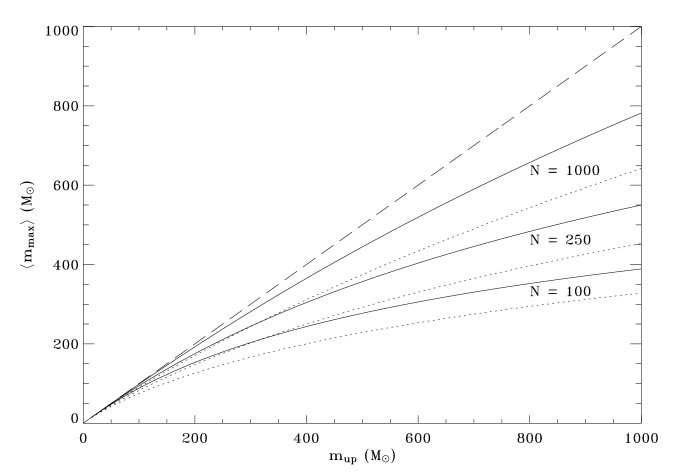
Figure 1.: Expected maximum mass $\langle m_{\rm max}\rangle$ vs upper-mass limit $m_{\rm up}$ of the parent distribution, for ensembles of $N_{*}=100,$ 250, and 1000 stars having masses $\geq 10\rm M_{\odot}$. Dotted lines assume the parent IMF has the form of a truncated Salpeter power law, and solid lines assume the form in equation 2. The dashed line shows the locus for $\langle m_{\rm max}\rangle=m_{\rm up}$.

The maximum stellar mass in the entire sample is around 120 – 150 M_⊙. We can compare this with the average expected maximum mass for an IMF with a Salpeter (1955) power-law slope $\gamma=2.35$, for an assumed upper-mass limit $m_{\rm up}$ of the parent distribution, and a given number of stars $N_{*}$ in the ensemble. As before, $N_{*}$ includes only stars of mass $m\geq 10$ M_⊙. The expected maximum mass $\langle m_{\rm max}\rangle$ is given by:

$$\langle m_{\rm max}\rangle=m_{\rm up}-\int_{0}^{m_{\rm up}}\Biggl{[}\int_{0}^{M}\phi(m)\ dm\Biggr{]}^{N}\ dM\quad.$$ (1)

Figure 1 shows the average expected $\langle m_{\rm max}\rangle$ as a function of $m_{\rm up}$ for three different values of $N_{*}$ (dotted lines). For a true upper-mass limit $m_{\rm up}=1000$ M_⊙, an ensemble having $N_{*}=250$ has an expected $\langle m_{\rm max}\rangle\sim 450$ M_⊙; an ensemble having $N_{*}=1000$ has $\langle m_{\rm max}\rangle\sim 650$ M_⊙. These values of $N_{*}$ are similar to those for our observed combined samples of Milky way and LMC associations, excluding and including R136a. We note that the values of $\langle m_{\rm max}\rangle$ do have some dependence on the assumed form of the parent IMF. The dotted lines in Figure 1 show the results from equation 1 for a simple Salpeter power-law truncated at $m_{\rm up}$. However, if we adopt a “softer” truncation of the form,

$$n(m)\ dm\propto\Biggl{[}\Biggl{(}\frac{m}{m_{\rm up}}\Biggr{)}^{-\gamma}-1\Biggr{]}\ dm\quad,$$ (2)

then instead equation 1 yields the solid lines in Figure 1.

In any case, as far as we know, no stars approaching these expected $m_{\rm max}$ values on the order of a few hundred M_⊙ are known to be observed, and the example calculations assume a true $m_{\rm up}$ of merely 1000 M_⊙, much less infinity. Indeed, inverting the argument, the observed values of $m_{\rm max}\sim 150$ M_⊙ imply that the parent $m_{\rm up}$ has a similar value. Elmegreen (2000) used this reasoning to estimate that if $m_{\rm up}=\infty$, then somewhere in the Milky Way, there should be a star having $m_{\rm max}$ = 10,000 M_⊙. No star remotely approaching this mass is suggested to have been seen.

However, given that the preceding is based on only 9 clusters, we may worry that, because of stochasticity, these may not be representative of the massive star population. We can quantify the degree to which we might be this unlucky by evaluating the probabilities $p(m_{\rm max})$ of obtaining the observed $m_{\rm max}$ seen in each cluster, for an assumed $m_{\rm up}$. Under normal circumstances, we should be uniformly lucky and unlucky, and so these $p(m_{\rm max})$ should represent a uniform distribution when $m_{\rm up}$ corresponds to its actual value in the parent distribution. Figure 2 shows the histograms of $p(m_{\rm max})$ for assumed $m_{\rm up}=10^{4}$, 200, 150, and 120 M_⊙. The probabilities $P$ that these histograms are drawn from uniform distributions for these respective cases are $P<0.002,\ <0.02,\ 0.12,$ and $<0.47$. Thus we confirm that, only when $m_{\rm up}$ has values similar to the observed $m_{\rm max}$, do we see significance in $P$, demonstrating that $m_{\rm up}$ in this particular sample is indeed around 150 M_⊙ at the significance implied by $P$. We note that Aban et al. (2006) point out that the statistical estimator for the maximum value of a truncated, inverse power-law distribution is indeed the maximum value in the dataset, corresponding to the observed $m_{\rm max}$.

It is especially remarkable that this apparent value of $m_{\rm up}\sim 150$ M_⊙ is seen over a great range in star-forming conditions. It holds for both ordinary OB associations in both the Milky Way, a massive, spiral galaxy; and the LMC, a lower-mass, irregular galaxy with presumably a lower-pressure ISM. At the same time, the same upper-mass limit applies in the R136a super star cluster, an extreme environment in the LMC. And Figer (2005) finds the same upper-mass limit in the Arches cluster near the Galactic Center, which is another extreme, yet very different, environment. We caution that these results are based on the inferred stellar masses for these systems, taken at face value, and assuming that the highest-mass stars have not yet expired.

Koen (2006) used the same dataset for R136a (Massey & Hunter 1998) to evaluate $m_{\rm up}$ and the IMF slope $\gamma$ from the cumulative stellar mass function. The cumulative distribution more clearly reveals the existence of a truncated $m_{\rm up}$. Koen simultaneously fit $m_{\rm up}$ and $\gamma$ for both sets of masses provided by Massey & Hunter, based on two different calibrations for spectral type to stellar effective temperature. The fit was carried out with both a least-squares method and a maximum likelihood method. Across all four cases, the results again are largely consistent with a Salpeter slope and $m_{\rm up}\sim 150$ M_⊙. Fixing $m_{\rm up}=\infty$ results in a very steep slope, $\gamma\sim 4$ to 5, strongly inconsistent with the Salpeter value. An infinite $m_{\rm up}$ is eliminated with a probability of $<0.0005$ and $<0.002$ for the least-squares and maximum-likelihood methods, respectively, consistent with our results (Oey & Clarke 2005).

3 Sparse OB Star Groups

Figure 2.: Histograms of $p(m_{\rm max})$ for assumed $m_{\rm up}=10^{4}$, 200, 150 and 120 M_⊙, as shown. For unbiased conditions, $p(m_{\rm max})$ should show a uniform distribution.

Given the apparent robustness of the upper-mass limit in a variety of local environments, we seek to examine other extreme circumstances. An especially interesting case is field OB stars. While a substantial fraction of these are likely to be runaway stars ejected from clusters, many may well be members of small, low-mass clusters. Oey et al. (2004) demonstrated that individual SMC field OB stars, as defined by a friends-of-friends algorithm, do fall smoothly on a continuous power-law distribution in the number of stars per cluster $N_{*}$, which is akin to the cluster mass function. This supports the scenario that most field OB stars are members of low-mass clusters.

We obtained F555W and F814W SNAP observations of eight, apparently isolated OB stars from among these SMC field stars, using the HST ACS camera (Lamb et al. 2010). Applying both a stellar density analysis and a friends-of-friends algorithm, we confirmed that three of these objects have stellar density enhancements, corresponding to sparse stellar groups. An additional object registered a positive signal for companions using the friends-of-friends algorithm, but not the stellar density analysis. The remaining four stars appear isolated to within the detection limit of F814W = 22 mag. Radial velocity observations subsequently revealed two of these stars to be runaway stars. This leaves two stars remaining as candidates for in-situ isolated, field OB stars.

We constructed Monte-Carlo simulations of cluster populations to examine the parameter space occupied by our observed, sparse OB star groups. We first adopted a cluster mass function (MF) given by a simple power-law distribution:

$$N(M_{\rm cl})\ dM_{\rm cl}\propto M_{\rm cl}^{-2}\ dM_{\rm cl}\quad,$$ (3)

where $N(M_{\rm cl})$ is the number of clusters in the mass range $M_{\rm cl}$ to $M_{\rm cl}+dM_{\rm cl}$. Each cluster drawn from this distribution is then populated with a stellar IMF drawn from a Kroupa (2001) IMF, which has the form,

$$n(m)\ dm\left\{\begin{array}[]{ll}m^{-1.3}\ dm\ ,\quad 0.08{\rm M_{\odot}}\leq m<0.5\ {\rm M_{\odot}}\\ m^{-2.35}\ dm\ ,\quad 0.5{\rm M_{\odot}}\leq m<150\ {\rm M_{\odot}}\end{array}\right.$$ (4)

We adopt a default model having a power-law index of –2 for the cluster MF (equation 3), and lower-mass limit of $M_{\rm cl,lo}=20$ M_⊙. This model best reproduces the frequency of single-O star clusters in the SMC and Milky Way (see Lamb et al. 2010).

Figure 3$a$ shows the mass ratio distribution of the second-highest to highest mass stars $m_{\rm max,2}/m_{\rm max}$ vs $m_{\rm max}$ in these simulations. Only clusters having a single OB star, defined in this figure as having mass $m\geq 18$ M_⊙ are shown. Our observed objects are overplotted with the black squares, showing upper limits for the apparently isolated objects. We see that while our observed objects appear to fall in a densely-populated region of the parameter space, the simulations peter out at the lowest values of $m_{\rm max,2}/m_{\rm max}$, since the probability of drawing an extremely low mass ratio is tiny. All of our data fall within the lowest 20th percentile in $m_{\rm max,2}/m_{\rm max}$, and these frequencies also result when our clusters are simulated based on cluster membership number $N_{*}$ instead of a MF (Figure 3$b$). This model analogously uses the form $N_{*}^{-2}$, the Kroupa IMF, and a lower limit of $N_{\rm*,lo}=40$ stars, which is equivalent to $M_{\rm cl,lo}$ used above. That our objects all fall in this low-frequency regime is partly due to our selection of apparently isolated OB stars as the HST targets. We note that the simulations reproduce this regime fairly easily.

Figure 4 shows the relation between the $m_{\rm max}$ and $M_{\rm cl}$ for the simulations based on the cluster mass function (equation 3), now showing all clusters having at least one OB star. Since there is no relation imposed between the $m_{\rm max}$ and $M_{\rm cl}$, the simulations occupy a large parameter space. The solid lines show the 10th, 25th, 50th, 75th, and 90th percentiles of $m_{\rm max}$ for a given $M_{\rm cl}$, and the dashed line shows the mean, equivalent to equation 1. Our observed objects are shown with the black squares as before, with $M_{\rm cl}$ computed by assuming that a fully populated IMF exists below the detection threshold of $\sim 1.5\ {\rm M_{\odot}}$. Open diamonds show the sample of observed clusters compiled by Weidner et al. (2010).

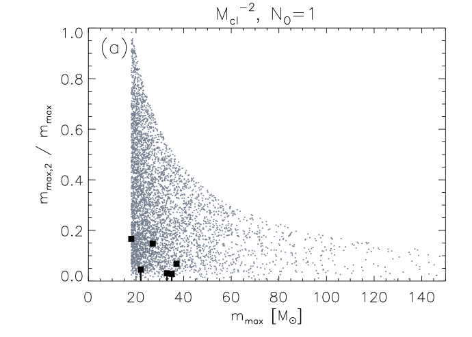
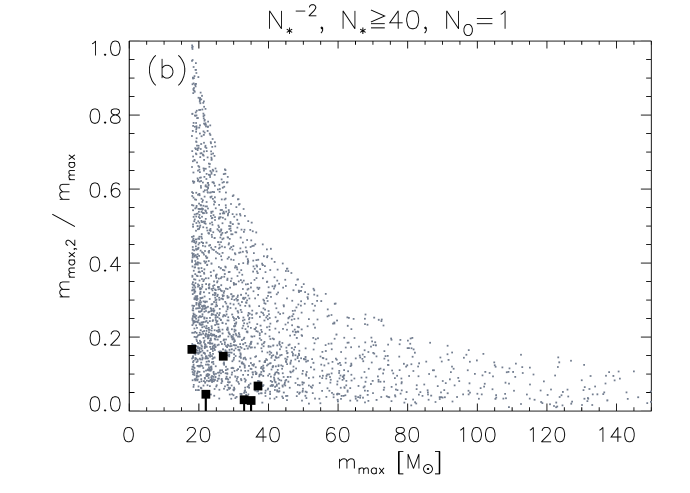
Figure 3.: Mass ratio of the two highest-mass stars vs $m_{\rm max}$ for cluster simulations based on a cluster MF (panel $a$; top) and on a cluster membership function (panel $b$; bottom). Only simulated clusters having a single OB star are shown, with gray points. Black squares correspond to our observed sparse O star groups, with three objects showing upper limits.

We see that for almost all of our observed objects, 90% of the simulated clusters have lower $m_{\rm max}$ for a given $M_{\rm cl}$, whereas the sample from Weidner et al. (2010) is largely at the opposite extreme. Our data, taken at face value, are in substantial conflict with the premise of a well-defined $m_{\rm max}$ – $M_{\rm cl}$ relation, proposed by Weidner & Kroupa (2005). The observed data show a scatter spanning two orders of magnitude in $M_{\rm cl}$ for the $m_{\rm max}$ in our sparse OB groups. While it is essential to understand the consequences of cluster dynamical evolution, this range in values, which is also consistent with the unconstrained simulations, strongly suggests that a $m_{\rm max}$ – $M_{\rm cl}$ relation is weak at best, as also found by Maschberger & Clarke (2008). Testi et al. (1999) discovered sparse groups around Galactic Herbig Ae/Be stars, which are newly formed objects, and thus their parent systems are unlikely to be strongly depleted by dynamical evaporation. Our observations extend such findings to OB stars.

The existence of a relation between $m_{\rm max}$ and $M_{\rm cl}$ is widely debated. A clear relation would strongly impact the integrated galaxy IMF (IGIMF; Weidner & Kroupa 2005), affecting interpretations of stellar populations, star-formation histories, and inferred galaxy evolution. Moreover, competitive accretion theories for star formation predict the existence of such a relation: $m_{\rm max}\propto M_{\rm cl}^{2/3}$ (Bonnell et al. 2004). It is therefore of great interest to further investigate whether sparse OB star groups are representative of their birth conditions.

4 Summary

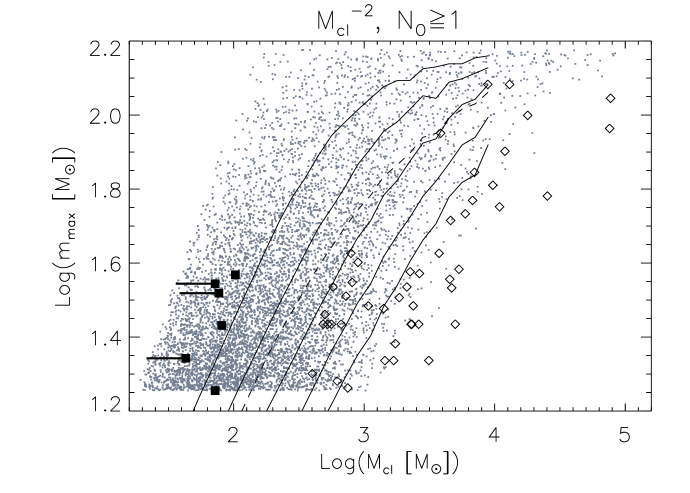
Figure 4.: $m_{\rm max}$ vs $M_{\rm cl}$ in simulations based on a cluster MF, for all objects with one or more OB stars. Our observed objects and the sample compiled by Weidner et al. (2010) are shown in black squares and open diamonds, respectively. Solid lines show the 10th, 25th, 50th, 75th, and 90th percentiles of $m_{\rm max}$, and the dashed line shows the mean.

With samples of uniformly derived OB star masses, we can begin to quantitatively evaluate the properties of the stellar upper IMF, based on a stochastic understanding of its nature. We demonstrated the existence of a stellar upper-mass limit $m_{\rm up}\sim 150$ M_⊙ for a Salpeter slope, using data for the massive star census in a sample of ordinary Milky Way and LMC OB associations, and the super star cluster R136a in 30 Doradus (Oey & Clarke 2005). Based the probability of observing the highest-mass stars in their respective clusters, we confirmed the existence of a strong deficit above this value of $m_{\rm up}$. Koen (2006) examined the cumulative distribution function of the stellar masses, and by jointly fitting $m_{\rm up}$ together with a power-law distribution for R136a, he confirmed a value for $m_{\rm up}\sim 150$ M_⊙ and a Salpeter-like slope as the best-fit values for these parameter estimations. The variety of environments in which this value of the upper-mass limit applies is remarkable: ordinary OB associations, the R136a super star cluster, and the Galactic Center environment.

To further examine the robustness of this upper-mass limit, we searched for low-mass companions around eight SMC field OB stars with HST/ACS. We confirmed the existence of sparse groups associated with 3 – 4 of these field massive stars, while 2 targets are runaway OB stars, and 2 – 3 remain candidates for isolated OB stars that formed in situ (Lamb et al. 2010). We generate Monte Carlo simulations of cluster populations based on simple power-law sampling for both cluster and stellar masses, and we find that the cluster lower-mass limit is most consistent with the frequency of SMC and Galactic field O stars at $M_{\rm cl,lo}\sim 20$ M_⊙ or $N_{\rm*,lo}\sim 40$ for a Kroupa IMF. Our sparse OB groups all fall in the lowest 20th percentile in $m_{\rm max,2}$/$m_{\rm max}$, regardless of whether the clusters are populated by $M_{\rm cl}$ or by $N_{*}$.

Our sparse OB groups generally fall in the highest 10th percentile of $m_{\rm max}$ for a given $M_{\rm cl}$, at an opposite extreme from the sample of objects compiled by Weidner et al. (2010), which fall in the locus of the most massive objects, at a given $m_{\rm max}$, in our simulations. Taken at face value, our results therefore contradict the existence of a well-defined relation between $m_{\rm max}$ and $M_{\rm cl}$. If our sample is not predominantly the result of dynamical evaporation, then this finding may pose difficulties for the predicted steepening of the IGIMF based on a suggested $m_{\rm max}$ – $M_{\rm cl}$ relation (e.g., Weidner & Kroupa 2005) and competitive accretion theories for star formation (Bonnell et al. 2004), which also rely on the existence of such a relation.

Acknowledgments

This work was supported by NASA HST-GO-10629.01 and NSF grant AST-0907758.

References

- Aban et al. (2006) Aban, I. B., Meerschaert, M. M., & Panorska, A. 2006, J. Am. Stat. Assoc, 101, 270
- Bonnell et al. (2004) Bonnell, I. A., Vine, S. G., & Bate, M. R. 2004, MNRAS, 349, 735
- Elmegreen (2000) Elmegreen, B. G. 2000, ApJ, 539, 342
- Figer (2005) Figer, D. F. 2005, Nat, 434, 192
- Koen (2006) Koen, C. 2006, MNRAS, 365, 590
- Kroupa (2001) Kroupa, P. 2001, MNRAS, 322, 231
- Lamb et al. (2010) Lamb, J. B., Oey, M. S., & Werk, J. K. 2010, ApJ, submitted
- Maschberger & Clarke (2008) Maschberger, T., & Clarke, C. J. 2008, MNRAS, 391, 711
- Massey & Hunter (1998) Massey, P., & Hunter, D. A. 1998, ApJ, 493, 180
- Massey et al. (1995) Massey, P., Johnson, K. E., & Degioia-Eastwood, K. 1995, ApJ, 454, 151
- Oey & Clarke (2005) Oey, M. S., & Clarke, C. J. 2005, ApJ, 620, L43
- Oey et al. (2004) Oey, M. S., King, N. L., & Parker, J. W. 2004, AJ, 127, 1632
- Salpeter (1955) Salpeter, E. E. 1955, ApJ, 121, 161
- Testi et al. (1999) Testi, L., Palla, F., & Natta, A. 1999, A&A, 342, 515
- Weidner & Kroupa (2005) Weidner, C., & Kroupa, P. 2005, ApJ, 625, 754
- Weidner et al. (2010) Weidner, C., Kroupa, P., & Bonnell, I. A. D. 2010, MNRAS, 401, 275