Linking haloes to galaxies: how many halo properties are needed?

Abstract

Recent studies emphasize that an empirical relation between the stellar mass of galaxies and the mass of their host dark matter subhaloes can predict the clustering of galaxies and its evolution with cosmic time. In this paper we study the various assumptions made by this methodology using a semi-analytical model (SAM). To this end, we randomly swap between the locations of model galaxies within a narrow range of subhalo mass ($M_{\rm infall}$). We find that shuffled samples of galaxies have different auto-correlation functions in comparison with the original model galaxies. This difference is significant even if central and satellite galaxies are allowed to follow a different relation between $M_{\rm infall}$ and stellar mass, and can reach a factor of $\sim 2$ for massive galaxies at redshift zero. We analyze three features within SAMs that contribute to this effect: a) The relation between stellar mass and subhalo mass evolves with redshift for central galaxies, affecting satellite galaxies at the time of infall. b) In addition, the stellar mass of galaxies falling into groups and clusters at high redshift is different from the mass of central galaxies at the same time. c) The stellar mass growth for satellite galaxies after infall can be significant and depends on the infall redshift and the group mass. All of the above ingredients modify the stellar mass of satellite galaxies in a way that is more complicated than a dependence on the subhalo mass only. By using two different SAMs, we show that the above is true for differing models of galaxy evolution, and that the effect is sensitive to the treatment of dynamical friction and stripping of gas in satellite galaxies. We find that by using the fof group mass at redshift zero in addition to $M_{\rm infall}$, an empirical model is able to accurately reproduce the clustering properties of galaxies. On the other hand, using the infall redshift as a second parameter does not yield as good results because it is less correlated with stellar mass. Our analysis indicates that environmental processes that affect galaxy evolution are important for properly modeling the clustering and abundance of galaxies.

1 Introduction

The current paradigm for the formation of structure in the Universe predicts that galaxies form and evolve inside of dark matter haloes. This working assumption makes the relation between the properties of galaxies and their host haloes a fundamental probe for various aspects of galaxy formation and cosmology. Galaxy properties such as stellar mass, star formation rate, color, and clustering are all intimately linked to the host halo mass. Consequently, there have been many recent attempts to quantify the relation between the mass of galaxies and their host halo mass (hereafter the ‘mass relation’).

Observational constraints on the mass relation were derived by weak lensing (e.g. Mandelbaum et al., 2006), satellite dynamics (e.g. Conroy et al., 2007) and large group catalogs of galaxies (Yang et al., 2009). All these are able to provide constraints on the stellar-halo mass relation for $10^{12}-10^{14}M_{\odot}$ haloes. At lower halo masses there are currently no useful direct observational constraints. Nonetheless, the abundance of low mass haloes is important for constraining the nature of dark matter (see, e.g. Bode et al., 2001; Macciò & Fontanot, 2010).

From the theoretical perspective, there are two main approaches for studying the relationship between stellar and halo masses. A straightforward way is to use existing models and extract the mass relation as a secondary result. This approach was demonstrated using hydrodynamical simulations (e.g. Sawala et al., 2010), and semi-analytical models (Wang et al., 2006; Moster et al., 2010). These two methodologies result in very different mass relations: hydrodynamical simulations predict higher stellar mass for a given halo mass, especially for low mass haloes. It is not clear whether the origin of this discrepancy is the different set of assumptions adopted by each model, the different observational data which are used to constrain the models, or some specific physical ingredients.

A different approach is to use the stellar-halo mass relation as the main assumption, and to verify it against a variety of observations. This approach is more useful for a systematic analysis of the mass relation, and for carefully testing the necessary ingredients needed to explain it. The halo occupation distribution (HOD) was historically the first approach to follow this line of thought (see Berlind & Weinberg, 2002; Tinker et al., 2005; Zehavi et al., 2005, and references therein). It assigns per each halo a specific number of galaxies of a given type. By tuning the parameters of the number and location distributions, these models are able to reproduce the abundance and clustering properties of galaxies. Thus, the relation between haloes and galaxies can be constrained using a relatively simple set of assumptions, and the halo mass is a sufficient parameter for fixing the properties of its galaxies.

Various studies have shown that the HOD approach can be simplified even more using information on the substructure within haloes, i.e., the subhalo mass (Kravtsov et al., 2004; Vale & Ostriker, 2004; Conroy et al., 2006; Shankar et al., 2006; Guo et al., 2010; Moster et al., 2010). In this approach, each subhalo can host only one galaxy. The galaxy mass is linked to the subhalo mass at the last time the subhalo was central within its fof group (hereafter $M_{\rm infall}$). The specific relation between stellar mass and $M_{\rm infall}$ is then fixed by matching the abundance of galaxies and $M_{\rm infall}$. This method is therefore termed ‘abundance matching’ (ABM; models based on the ABM approach will be termed ABMs in what follows). Using subhalo samples from large cosmological $N$-body simulations, ABMs are able to reproduce the auto-correlation function of galaxies surprisingly well. The main difference between the HOD and the ABM approach is thus that HOD uses the fof mass for determining stellar masses, while the ABM approach uses the subhalo mass, which is limited to contributions from smaller scales of dark matter.

By fixing the stellar mass according to $M_{\rm infall}$ only, ABMs assume various simplifications to the statistics of galaxy formation. First, they neglect the redshift where the galaxy became a satellite. This redshift should affect the stellar mass because the mass relation evolves with redshift. Second, the stellar mass gained by satellite galaxies after infall is assumed to be independent of clustering. Third, ABMs do not allow a galaxy’s large-scale environment to modify its stellar mass (Croton et al., 2007). However, it seems that these simplifications do not force the models to violate the clustering properties of galaxies. It is not clear if this is due to the low sensitivity of the auto-correlation function to these assumptions, or because multiple effects conspire to cancel each other and leave the auto-correlation function unchanged.

In this paper we will test the ABM assumptions using detailed semi-analytical models (hereafter SAMs). We will test whether the stellar mass function and clustering of galaxies in the SAMs depend only on $M_{\rm infall}$. It will be shown that SAMs do not follow the above assumptions made by ABM models. The inclusion of more detailed physics, and the fact that SAMs follow the evolution of each individual galaxy, affects the auto correlation functions of the model galaxies. The success of ABMs thus poses important questions on the processes which govern galaxy formation. Is it possible that the simple ABM approach mimic the observed clustering better than the more sophisticated models? Or is their success purely a coincidence?

In order to compare ABMs to SAMs we will use the technique of shuffling between the location of model galaxies. This method was introduced by Croton et al. (2007), as a tool to quantify the effect of large-scale environment on the stellar mass of galaxies. These authors found that environment of the host fof halo can contribute up to $\sim 10$ per cent variation in the correlation function of galaxies. Here we adopt a similar technique in order to test the role of $M_{\rm infall}$ in shaping the stellar mass of galaxies and their correlation function. The effect we find is an order of magnitude larger than the one found by Croton et al. (2007) at least for high mass galaxies. This is because Croton et al. (2007) test the HOD model, and not ABM, which means that they shuffle galaxies between fof groups and not between subhaloes.

One of the targets of this paper is to suggest possible ingredients for more detailed ABM studies. We would like to find which ingredients might contribute to the clustering of galaxies, independent of the specific model chosen here. This will allow future ABM studies to fully explore the parameter space. For this reason, we use models that span a large range of possible physical recipes. The two basic SAMs we use in the work are taken from Neistein & Weinmann (2010), which discusses six different specific models spanning a large range of galaxy formation scenarios.

This paper is organized as follows. In section 2 we describe the two different methodologies used in this work, namely ABMs and SAMs. The shuffling test, which reveals deviations between ABMs and SAMs, is discussed in section 3. Section 4 is devoted to a more systematic analysis of the various differences between the two methodologies. In section 5 we then suggest an extension to ABMs that is able to reproduce the results of SAMs. Lastly, we summarize the results and discuss them in section 6.

This paper is based on the cosmological model with $(\Omega_{\rm m},\,\Omega_{\Lambda},\,h,\,\sigma_{8})=(0.25,\,0.75,\,0.73,\,0.9)$, which is the model adopted by the Millennium simulation used here (Springel et al., 2005). Mass units are $M_{\odot}$ unless otherwise noted; Log designates Log₁₀.

2 Methodologies

2.1 Abundance matching

Abundance matching models (ABMs) link the stellar mass of a galaxy to its host subhalo mass using a simple and empirical methodology. The ingredients of the models can be summarized as follows:

1. Subhalo selection and mass definition: here we choose which subhaloes are allowed to host galaxies, and how their mass is defined. As a result, the abundance of subhaloes and their locations are set.

2. Assume a one-to-one relation between the subhalo mass and the stellar mass of its galaxy: $m_{\rm star}-M_{\rm infall}$. More complex models allow scatter, or use different relations for satellite and central galaxies.

3. Solve for the $m_{\rm star}-M_{\rm infall}$ relation, in order to reproduce the observed stellar mass function.

For simplicity, we discuss ABMs which are aimed at producing a population of galaxies at $\emph{z}=0$ only. Such models are usually tested against the auto-correlation function of galaxies at $\emph{z}=0$ (see §2.2.4 below). For a detailed review of ABMs and the various uncertainties involved see Behroozi et al. (2010). In this section we further explain the various ingredients of ABMs and specify the actual model assumed here.

We first define the subhalo mass, $M_{\rm infall}$, which will be used later in order to fix the stellar mass of galaxies:

$$M_{\rm infall}=\left\{\begin{array}[]{ll}M_{h}&\textrm{if central within its {fof~{}}group}\\ &\\ M_{h,p}(\emph{z}_{\rm infall})&\textrm{otherwise}\end{array}\right.$$ (1)

Here $\emph{z}_{\rm infall}$ is the lowest redshift at which the main progenitor of the subhalo $M_{h}$ was the central of its fof group, and $M_{h,p}$ is the main progenitor mass at this redshift. We select all the subhaloes from the Millennium simulation (Springel et al., 2005, see section 2.2.1) at $\emph{z}=0$. Unlike many ABMs, we also consider subhaloes that are not identified at $\emph{z}=0$ if their galaxies survive within the SAM and did not have enough time to merge with the central galaxy. Even though these subhaloes are only identified at high redshift, their $M_{\rm infall}$ can still be computed according to Eq. 1.

The basic assumption of ABMs (e.g. Conroy et al., 2006) is listed in item (ii) above: the stellar mass of a galaxy depends solely on $M_{\rm infall}$. Most ABMs assign a unique $m_{\rm star}$ value per each subhalo mass. However, several studies allow a scatter in the mass relation, and Wang et al. (2006) use different relations for central galaxies versus satellite galaxies (the mass relations are adopted from the results of a SAM in this last case). In this work we mainly discuss the most detailed ABM approach, where the $m_{\rm star}-M_{\rm infall}$ relation includes scatter, and might be different for satellite galaxies. We will show that even when using this extended approach, the SAM behaviour is different from ABMs.

Once the assumption on the nature of the $m_{\rm star}-M_{\rm infall}$ relation has been made, the last step in constructing the model is to find a relation $m_{\rm star}-M_{\rm infall}$ that will reproduce the observed abundance of $m_{\rm star}$. If all the subhaloes from item (i) are populated with galaxies according to this relation, the resulting set of galaxies would have the observed stellar mass function by construction. The $m_{\rm star}-M_{\rm infall}$ relation can be thus obtained if one assumes that it follows some general functional shape, where the free parameters are constrained by matching the $m_{\rm star}$ abundance. A different solution can be obtained by solving for the numerical values for $m_{\rm star}-M_{\rm infall}$ in each mass bin separately. In this work we do not assume any functional shape a-priori, but rather adopt the same $m_{\rm star}-M_{\rm infall}$ relation as in the SAMs.

Although ABMs seem to adopt a rather simplified set of assumptions, it turns out that the clustering properties of galaxies fit the observational data well. This is encouraging, as clustering is the main test of the model (stellar mass functions are reproduced by construction). In addition, it was shown by Wang et al. (2006) that the results of a specific SAM agrees quite well with this approach. All of these tests indicate that ABMs provide a reasonable solution to the relation between halo mass and stellar mass. It is not clear, however, whether this relation is the only possible solution.

2.2 The Semi-analytical models

In this section we briefly describe the SAM formalism being used in this work for modeling the evolution of galaxies. For more details the reader is referred to Neistein & Weinmann (2010) (hereafter NW10). A version of the code used in this work is available for public usage through the internet (at http://www.mpa-garching.mpg.de/galform/sesam).

2.2.1 Merger trees

We use merger trees extracted from the Millennium $N$-body simulation (Springel et al., 2005). This simulation was run using the cosmological parameters $(\Omega_{\rm m},\,\Omega_{\Lambda},\,h,\,\sigma_{8})=(0.25,\,0.75,\,0.73,\,0.9)$, with a particle mass of $8.6\times 10^{8}\,\,h^{-1}{M_{\odot}}$ and a box size of 500 $h^{-1}$Mpc. The merger trees used here are based on subhaloes identified using the subfind algorithm (Springel et al., 2001). They are defined as the bound density peaks inside fof groups (Davis et al., 1985). More details on the simulation and the subhalo merger-trees can be found in Springel et al. (2005) and Croton et al. (2006). The mass of each subhalo (referred to as $M_{h}$ in what follows) is determined according to the number of particles it contains. Within each fof group the most massive subhalo is termed the central subhalo of its group.

2.2.2 Quiescent evolution

Each galaxy is modeled by a 4-component vector,

$${\bf m}=\left(\begin{array}[]{c}m_{\rm star}\\ m_{\rm cold}\\ m_{\rm hot}\\ m_{\rm eject}\end{array}\right)\,,$$ (6)

where $m_{\rm star}$ is the mass of stars, $m_{\rm cold}$ is the mass of cold gas, $m_{\rm hot}$ is the mass of hot gas distributed within the host subhalo, and $m_{\rm eject}$ is the mass of gas which is located out of the subhalo and is not able to cool directly into the cold phase. We use the term ‘quiescent evolution’ to mark all the evolutionary processes of a galaxy except those related to mergers.

It can be shown (see NW10) that most of the quiescent processes included in SAMs can be written in a compact form by using linear differential equations. We therefore adopt the following model for the quiescent evolution:

$$\dot{{\bf m}}={\bf A}{\bf m}+{\bf B}\dot{M}_{h}\,,$$ (7)

where $\dot{M}_{h}$ is the growth rate of the subhalo mass due to smooth accretion (i.e., mass which does not come within other subhaloes), and

$${\bf A}=\left(\begin{array}[]{cccc}0&(1-R)f_{\rm s}&0&0\\ 0&-(1-R)f_{\rm s}-f_{\rm d}f_{\rm s}&f_{\rm c}&0\\ 0&f_{\rm d}f_{\rm s}-f_{\rm e}f_{\rm s}&-f_{\rm c}&f_{\rm re}\\ 0&f_{\rm e}f_{\rm s}&0&-f_{\rm re}\end{array}\right)$$ (12)

$${\bf B}=\left(\begin{array}[]{c}0\\ 0\\ 0.17\\ 0\end{array}\right)\,\,.$$ (17)

In short, $f_{\rm s},\,f_{\rm c},\,f_{\rm d},\,f_{\rm e},\,f_{\rm re}$ are all functions of subhalo mass and redshift, and correspond to the efficiencies of star-formation, cooling, feedback, ejection, and reincorporation respectively. $R$ is the constant recycling factor, which has the values of $0.43$ or $0.5$ in all the models used in this work.

2.2.3 Satellite galaxies: dynamical friction, stripping, and bursts

Satellite galaxies are defined as all galaxies inside a fof group except the main galaxy inside the central (most massive) subhalo. Once the subhalo corresponding to a given galaxy cannot be resolved anymore, it is considered as having merged into the most massive subhalo which has the same descendant (the ‘target’ subhalo). Due to the effect of dynamical friction, the galaxy is then assumed to spiral towards the center of the target subhalo, and merge with the central galaxy in that subhalo after a (potentially significant) delay time. We thus divide galaxies into three different types:

$$\textrm{galaxy type}=\left\{\begin{array}[]{ll}0&\textrm{if central within its {fof~{}}group}\\ 1&\textrm{if central within its subhalo (`satellite')}\\ 2&\textrm{otherwise (`satellite')}\end{array}\right.$$ (18)

Galaxies of type 0 and 1 can serve as merging targets for type 2 galaxies. A type 2 galaxy is not following the evolution of its original host subhalo, as its subhalo is not identified anymore. Consequently, type 2 galaxies do not have a well defined location given by the simulation data. We estimate the location of these galaxies by using the location of the most bound particle of the last identified subhalo. This method was used before by e.g. Croton et al. (2006); Guo et al. (2010).

In our model, the time it takes the galaxy to fall into the central galaxy is determined by dynamical friction, and is not directly related to the true evolution of the location of the most bound particle with respect to its target. At the last time the dark matter subhalo of a satellite galaxy is resolved we compute its distance from the target subhalo ($r_{\rm sat}$), and estimate the dynamical friction time using the formula of Binney & Tremaine (1987),

$$t_{\rm df}=\alpha_{\rm df}\cdot\,\frac{1.17V_{v}r_{\rm sat}^{2}}{Gm_{\rm sat}\ln\left(1+M_{h}/m_{\rm sat}\right)}\,.$$ (19)

Here $M_{h}$ is the mass of the target subhalo and $V_{v}$ is its virial velocity. The value of $m_{\rm sat}$ should correspond to the mass of the satellite galaxy which is affected by the dynamical friction process. We use two options for $m_{\rm sat}$ as listed below:

$$m_{\rm sat}=\left\{\begin{array}[]{ll}m_{\rm star}+m_{\rm cold}+M_{h,min}&(a)\\ M_{h}&(b)\,\,.\end{array}\right.$$ (20)

Here $M_{h,min}$ is the minimum subhalo mass of the Millennium simulation ($1.72\times 10^{10}\,h^{-1}{M_{\odot}}$), and $M_{h}$ is the last subhalo mass identified, just before the subhalo has merged into a bigger one. In addition to the freedom in choosing $m_{\rm sat}$, a free parameter, $\alpha_{\rm df}$, was added to Eq. 19 in order to easily modify the dynamical friction time. When a satellite falls into a larger subhalo together with its central galaxy we update $t_{\rm df}$ and the target subhalo, for both objects according to the new central galaxy.

While satellite galaxies move within their fof group, they suffer from mass loss due to tidal stripping. Only the ejected and hot gas of the satellite can be stripped in our model. We assume that this stripping has an exponential dependence on time, using the same time scale for all galaxies. In order to model this stripping we modify ${\bf A}$ by subtracting a constant $\alpha_{h}$ from two of its elements:

$${\bf A}_{sat}(3,3) = -f_{\rm c}-\alpha_{h}$$ (21)

$${\bf A}_{sat}(4,4) = -f_{\rm re}-\alpha_{h}\,.$$

This constant suggests an exponential decrease in the amount of hot and ejected gas. However, the actual dependence of these components on time is more complicated due to contributions from other processes, as seen in Eq. 17.

When satellite galaxies finally merge we assume that a SF burst is triggered. We follow Mihos & Hernquist (1994); Somerville et al. (2001); Cox et al. (2008) and model the amount of stars produced by

$$\Delta m_{\rm star}=\alpha_{b}\left(\frac{m_{1}}{m_{2}}\right)^{\alpha_{c}}(m_{1,{\rm cold}}+m_{2,{\rm cold}})\,.$$ (22)

Here $m_{i}$ are the baryonic masses of the progenitor galaxies (cold gas plus stars), $m_{i,{\rm cold}}$ is their cold gas mass, and $\alpha_{b}$, $\alpha_{c}$ are constants.

2.2.4 Correlation functions

In this paper we study the clustering properties of various models using the projected auto-correlation function, $w_{p}(r_{p})$, termed CF hereafter. Observational data were obtained from the full SDSS DR7 release, using 1/Vmax weighting, in the same method as described in Li et al. (2006) and presented in Guo et al. (2010). Errors are estimated from a set of 80 mock SDSS surveys mimicking cosmic variance effects. The CFs are split into five stellar mass bins, and are plotted as error-bars in Fig. 1 (the same data points are used throughout this work).

In order to compute $w_{p}(r_{p})$ for the models, we use only two coordinates for the location of model galaxies (i.e. $r_{x},r_{y}$, omitting the $r_{z}$ dependence). We then count the number of galaxy pairs, $N_{p}$, within the same stellar mass bin, and at a given separation $r_{p}$ ($r_{p}=\sqrt{r_{x}^{2}+r_{y}^{2}}$). The CF is computed from $N_{p}$ using:

$$w_{p}(r_{p})=\left[\frac{L^{2}}{N^{2}}\frac{N_{p}}{V_{p}}-1\right]L\,.$$ (23)

Here $V_{p}$ is the 2-dimensional area covered by the bin $r_{p}$, $N$ is the total number of galaxies in the sample, and $L$ is the size of the simulation box in $h^{-1}$Mpc. The resulting $w_{p}(r_{p})$ has units of $h^{-1}$Mpc. In order to save computational time, we compute CFs only for a random subset of 10 per cent of the galaxies within the lower three mass bins (we use all galaxies for the two most massive bins). We checked that there is no difference between the CF computed using the partial sample and the full sample from the Millennium simulation used here.

2.2.5 Specific models

Table 1: The different SAM models used in this paper. The models are divided into two groups, $A$ & $B$. Within each group the specific models are the same except the details given in this table. Different $m_{\rm sat}$ mass estimates for computing dynamical friction are given in Eq. 20. Model $A4$ evolves satellite galaxies according to Weinmann et al. (2010)

Name	$\alpha_{h}^{-1}$ [Gyr]	$\alpha_{\rm df}$	$m_{\rm sat}$	Other
$A0$	4	3	a
$A1$	0	3	a	no stellar growth for satellites
$A2$	0.01	2	b
$A4$	4 (for type 2)	0.3	b	Weinmann et al. (2010)
$B0$	0.01	2	b
$B1$	0	2	b	no stellar growth for satellites
$B2$	4	3	a

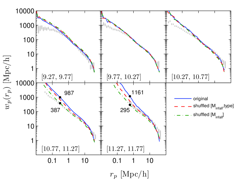
Figure 1: The projected auto-correlation functions derived for model $A0$. Each panel corresponds to galaxies with stellar masses as indicated by the range of Log$M_{\odot}$. Solid lines show the results of the original model, dashed lines are plotted using shuffling within [$M_{\rm infall}$,type], dashed-dotted lines represent shuffling within [$M_{\rm infall}$] only. See §3 for more information about the shuffling procedure. The observational data are using SDSS DR7 with the same technique as in Li et al. (2006), and are shown as error bars. In the two most massive bins we add labels for the y-axis values of the corresponding line. Poisson errors for the model results are smaller than 10 percent for all points, and would not be visible in this plot.

We choose to examine the results of two models which were originally presented in NW10. Other models from NW10 have similar results and are not adding a significant information to this work. We use model II from NW10, in which SF, feedback, and mergers are treated in a similar way as in standard SAMs. Three main modifications to usual SAMs are adopted in this model: i) There is no ejection of gas out of the subhalo ($m_{\rm eject}\equiv 0$); ii) the SF law does not include a threshold in cold gas density; iii) Cooling rates ($f_{\rm c}$) are tuned to reproduce a large set of observational data. This model will be termed model $A0$ in this paper. The second model being used here is the one based on De Lucia & Blaizot (2007) (model 0 in NW10), and is termed model $B0$.

There are a few differences between the results of models $A0$ and $B0$ that are important for the following sections. The stellar mass functions of these models are very different (see Fig. 10 in the Appendix). Model $A0$ fits the observed stellar mass functions for $\emph{z}<3$, while model $B0$ shows significant deviations at low and high masses. We will see below that this difference affects the relation between the subhalo mass and stellar mass, and the CFs. The treatment of satellite galaxies is also different between these models. The dynamical friction and stripping time-scales are longer in model $A0$. Consequently, satellite galaxies survive longer, and are able to form a significant amount of stars after joining the group. Longer dynamical friction time-scales also result in more galaxies of type 2 in model $A0$.

As we will show later in this work, the results of the CFs are sensitive to the treatment of dynamical friction and gas stripping in satellite galaxies. In order to further investigate these effects we run a few variations of the original models. Models $A1$,$B1$ are the same as models ‘0’ except that satellite galaxies are not allowed to grow in their stellar mass. We artificially shut down all modes of SF and do not allow merging into galaxies of type 1 & 2. These models mimic extremely fast stripping mechanisms.

In models $A2$,$B2$ we exchange the recipes of dynamical friction and stripping between models $A0$ & $B0$, showing the effect of these ingredients on the results. This will help us disentangle between the effects of quiescent evolution, and treatment of satellites.

Lastly, in model $A4$, we use a prescription for the evolution of satellite galaxies as proposed by Weinmann et al. (2010). In this model gas stripping follows the stripping of the subhalo mass (as calculated from the $N$-body simulation), where the first quantity to be stripped is $m_{\rm eject}$. Only when $m_{\rm eject}$ reaches zero does stripping of the hot gas start. For type 2 galaxies, we use exponential stripping of hot gas, using $\alpha_{h}$ defined in Eq. 2.2.3 above. Model $A4$ was developed in order to match in detail the properties of satellite galaxies, and is thus the most physically motivated model here, in terms of environmental effects within the halo. When tuning the dynamical friction time scale in Model $A4$ we have tried to better reproduce the observed CFs (see Fig.9 in the Appendix).

Table 1 summarizes the various models used in this work.

3 The shuffling test

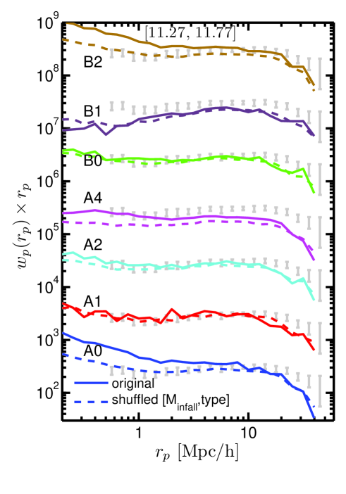
Figure 2: The projected auto-correlation function for the models listed in Table 1. Only galaxies with stellar mass $11.27\leq m_{\rm star}\leq 11.77$ Log$M_{\odot}$ are selected (corresponding to the most massive stellar bin in Fig. 1). Solid lines are the original (un-shuffled) CFs. Dashed lines show the shuffling results of each model (shuffling is preformed within galaxies of the same $M_{\rm infall}$ and type). The CFs of different models are multiplied by powers of 10 for clarity.

We want to check whether SAMs include some clustering information that is lost by the assumptions of ABM. A simple test to this problem is to adopt the same $m_{\rm star}-M_{\rm infall}$ relation as in the SAM, and use it within an ABM application. Such a test was done by Wang et al. (2006). Here we choose to use the shuffling procedure for testing ABMs against SAMs. In general, we will randomly re-distribute the location of SAM galaxies with the same $M_{\rm infall}$. In this way we mimic an ABM model with the same subhaloes as used in the SAM, and with exactly the same distribution of $m_{\rm star}$ per a given $M_{\rm infall}$. Information about the clustering of galaxies that is not related to $M_{\rm infall}$ should be eliminated by this procedure, and its effect on the CFs can be easily tested without modeling the specific $m_{\rm star}-M_{\rm infall}$ relation. Moreover, it will be easy to see how different modifications of SAMs behave under shuffling, and to add constraints on the shuffled groups.

We first run the SAMs and construct a catalog of galaxies at $\emph{z}=0$. For each galaxy we save its location at $\emph{z}=0$, its type (0/1/2, see Eq. 18), its host $M_{\rm infall}$, the infall redshift $\emph{z}_{\rm infall}$, and the host fof group mass at $\emph{z}=0$, $M_{\rm 200}$. We then split the population of galaxies into groups of the same $M_{\rm infall}$. Within each group of galaxies we randomly re-distribute the stellar masses at the group locations. In order to further explore the clustering properties of SAMs, we will refer in this work to a few versions of shuffling:

• Shuffling within [$M_{\rm infall}$]

• Shuffling within [$M_{\rm infall}$,type]

• Shuffling within [$M_{\rm infall}$,type,$\emph{z}_{\rm infall}$]

• Shuffling within [$M_{\rm infall}$,type,$M_{\rm 200}$]

In each case we split the catalog of galaxies into groups where the values of the variables listed in square brackets are the same . The shuffling is then implemented in each group separately. When computing the CF for massive galaxies, we always run 20 different random realizations of shuffling, and plot the average CF values.

In Fig. 1 we compare the CFs of model $A0$ against two basic shuffling tests. When we shuffle between all galaxies of the same $M_{\rm infall},$ the resulting difference in the CF is very large. It reaches a factor of $\sim 4$ in the most massive bin, and a factor of $\sim 2.5$ in the second most massive bin. These large differences indicate that treating satellite and central galaxies with the same $m_{\rm star}-M_{\rm infall}$ relation does not agree with SAMs. We will show below that the $m_{\rm star}-M_{\rm infall}$ relation for central galaxies is very similar to that for satellites in all of the models used here when considering low-mass galaxies. This is probably the reason why the CFs at the low mass bins do not show a change after shuffling. In this paper we do not attempt to reproduce the observed CFs (except for model $A4$ as explained above), but rather compare the results of different models. Thus, the observational data presented in Fig. 1 are only meant to provide a basis for comparison between the models. There is probably no special meaning to the fact that the shuffled samples better agree with the observed CFs.

Interestingly, the model shows significant change in the CF at the higher stellar mass bin, even when performing shuffling within $[M_{\rm infall}$,type$]$. This difference reaches a factor of $\sim 2$ at small scales. More minor differences are apparent in the other mass bins, at the level of 15 to 40 per cent. These differences indicate that the SAM contains clustering information that depends on something other than $M_{\rm infall}$ and galaxy type.

We have tested the effect of shuffling within $[M_{\rm infall}$,type$]$ on all the models listed in Table 1 and found that variations between the different models are relevant mainly for the most massive stellar mass bin. We therefore show the CFs for this bin, and for all the models, in Fig. 2. Some models do not show any difference between the original and the shuffled samples, while other models exhibit substantial differences. Consequently, model $A0$ is not unique in showing differences in CFs due to shuffling. Although model $B0$ does not include any change in the CFs (in agreement with Wang et al., 2006), changing the dynamical friction and stripping time-scales in model $B2$ introduces a change in the CFs due to shuffling.

In order to find the reason for the behaviour of the shuffled catalogs we first did the following tests:

1. We shuffled only galaxies with one specific type, leaving all other type of galaxies unchanged. The results of this test are that only galaxies of type 1 & 2 contribute to the shuffling difference. Central (type 0) galaxies do not change their clustering properties because of shuffling. We will therefore examine below mechanisms which affect the evolution of satellite galaxies.

2. We tested different definitions of the host subhalo mass instead of $M_{\rm infall}$: the maximum mass in the history of the subhalo, and the mass at the first infall identified by the simulation (our usual definition of $M_{\rm infall}$ is at the lowest redshift where the subhalo was identified as central, i.e. the last infall). All these definitions give rise to the same CF sensitivity under shuffling.

In the next section we will discuss the various differences between SAMs and ABMs in order to better understand the possible reasons for the effect of shuffling on the CFs.

4 Differences between ABM & SAM

The results of the shuffling test shown in the previous section indicate that galaxies produced by ABMs cluster differently than SAM galaxies. In order to further study this effect we closely follow each of the assumptions made by ABMs and see if it is fulfilled by our SAMs. Our motivation is to study second order effects, which are currently not being used by ABMs, that contribute to the clustering properties of galaxies.

4.1 Mass function of subhaloes

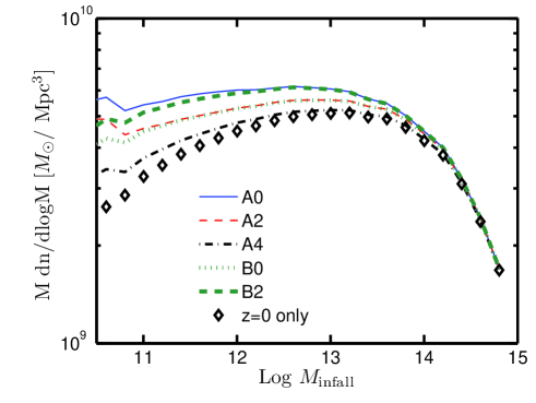
Figure 3: The abundance of subhaloes with mass $M_{\rm infall}$, obtained by assigning $M_{\rm infall}$ for each galaxy from the SAM catalog at $\emph{z}=0$. For type 2 galaxies, we assign $M_{\rm infall}$ according to the subhalo in which these galaxies were last identified as type 1 or 0. Different line types correspond to different specific SAMs, as listed in Table 1. The diamond symbols show the abundance of $M_{\rm infall}$ for subhaloes which are identified at $\emph{z}=0$ only.

ABMs often consider subhaloes which are identified at the inspected redshift only (i.e. at $\emph{z}=0$). Although modern high-resolution cosmological simulations seem to resolve substructure well enough (Conroy et al., 2006; Moster et al., 2010; Guo et al., 2010), there is still some uncertainty whether this resolution is adequate (Guo et al., 2010). On the other hand, SAMs follow galaxies even if their host subhalo has already merged into a bigger one. This is done by allowing galaxies to survive an additional time inside their host halo according to dynamical friction estimates (see §2.2.3). As a result, the number of galaxies at $\emph{z}=0$ in the SAMs might be significantly higher than the number of subhaloes at the same redshift, where the additional galaxies are all marked as type 2.

In order to quantify this effect we assign $M_{\rm infall}$ for each galaxy in the SAM catalog at $\emph{z}=0$, as was explained in section 2.1. For type 2 galaxies we use $M_{\rm infall}$ according to the subhalo when the galaxy was last identified as type 0 or 1. The resulting mass functions for all the models are plotted in Fig. 3. It is evident that all of the SAMs contain a non-negligible number of type 2 galaxies at $\emph{z}=0$. In models that use a long dynamical friction time scale, the difference is bigger, and can be significant even at masses that are two orders of magnitude above the minimum mass of the simulation.

Although the difference in the number of galaxies is sometimes small in comparison to the total population, these type 2 galaxies might still affect the CF. In particular, such galaxies are usually located close to the central galaxies of their fof group, and thus contribute to the CF at small scales, where a small number of galaxies can make a significant difference. The effect can be seen by comparing the CF of model $A0$ against model $A4$ (Fig. 2). These models mainly differ in the way dynamical friction is modeled, resulting in a significant change in the CF at small scales.

The shuffling test done here does not change the number of type 2 galaxies so different mass functions of $M_{\rm infall}$ do not affect this test directly. This can be seen when comparing Fig. 2 and 3, there is no obvious correlation between models that are sensitive to shuffling and models with high abundance of $M_{\rm infall}$.

4.2 Redshift dependence

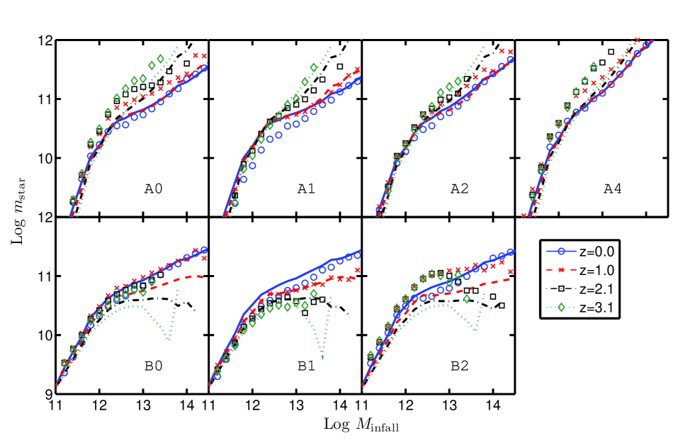
Figure 4: The $m_{\rm star}-M_{\rm infall}$ relation for the various models used in this work and for different redshifts. Each panel shows results from a specific model as listed in Table 1. All the values of $m_{\rm star}$ were derived by computing the average per a given $M_{\rm infall}$ mass bin. Lines show $m_{\rm star}$ for type 0 galaxies which are selected at the indicated redshift. Symbols show $m_{\rm star}$ for type 1 & 2 galaxies identified at $\emph{z}=0$, split according to their infall redshift $\emph{z}_{\rm infall}$. For type 1 & 2 galaxies, we allow $\emph{z}_{\rm infall}$ to deviate in $\Delta\emph{z}=\pm 0.2$ from the indicated z label ($\Delta\emph{z}=\pm 0.5$ for $\emph{z}=3$).

In Fig. 4 we show the $m_{\rm star}-M_{\rm infall}$ relation for the SAMs used here for various redshifts. Clearly, the relation between stellar mass and subhalo mass depends on redshift for central galaxies, as was found by previous ABM studies (e.g., Conroy & Wechsler, 2009). This dependence is mainly related to the evolution of the stellar mass functions with redshift. At the massive end, the average $m_{\rm star}-M_{\rm infall}$ relation is also affected by the scatter in $m_{\rm star}$ for a given value of $M_{\rm infall}$. For low mass galaxies, all the models show little or no evolution with redshift, in contrast to the relation derived by Conroy & Wechsler (2009). This might be a consequence of the different stellar mass functions used by these authors. A different important point to note is that the $A$ models show very different behaviour than the $B$ models. This difference is an outcome of the stellar mass function and its evolution with redshift. The $B$ models produce too many small mass and high mass galaxies, so their $m_{\rm star}-M_{\rm infall}$ relations are probably incorrect.

The dependence on redshift, which is rather obvious for central galaxies (smooth lines in Fig. 4), is also important for satellite galaxies identified at $\emph{z}=0$. In Fig. 4 we plot the average $m_{\rm star}$ for satellite galaxies with different $\emph{z}_{\rm infall}$ as symbols. In the $A$ models, galaxies with higher infall redshift have higher current stellar mass, while the $B$ models show the opposite trend. This effect is not included in current ABMs when matching the $m_{\rm star}-M_{\rm infall}$ relation at redshift zero. Shuffling between satellite galaxies of the same $M_{\rm infall}$ will mix galaxies of different $\emph{z}_{\rm infall}$, an effect that might change the CF and contribute to the differences shown in Fig. 2.

We note that the average $m_{\rm star}$ per a given $\emph{z}_{\rm infall}$ seen in Fig. 4 does not provide enough information in order to quantify the effect of shuffling, as it does not include information on the number of galaxies per each $\emph{z}_{\rm infall}$. The population of satellite galaxies is dominated by low values of $\emph{z}_{\rm infall}$, so only values of $\emph{z}_{\rm infall}\lesssim 1$ are relevant. This issue will be further examined in section 5.

4.3 Evolution at early times

In the previous section we discussed the correlation between $\emph{z}_{\rm infall}$ and $m_{\rm star}$ for satellite galaxies, and for a given $M_{\rm infall}$. However, the average $m_{\rm star}$ for satellite galaxies at $\emph{z}=0$ with a specific $\emph{z}_{\rm infall}=\emph{z}_{0}$ is different from the $m_{\rm star}$ of central galaxies at the same $\emph{z}_{0}$. This is seen by comparing lines and symbols in Fig. 4. As a result, one cannot use the $m_{\rm star}-M_{\rm infall}$ relation that was derived for central galaxies at high-redshift (e.g., Conroy & Wechsler, 2009), in order to model the $m_{\rm star}-M_{\rm infall}$ for satellites at $\emph{z}=0$ with various $\emph{z}_{\rm infall}$. Here we will explore one reason for this effect, namely the difference in $m_{\rm star}$ at the time of infall. In the next section we will study the growth in $m_{\rm star}$ after $\emph{z}_{\rm infall}$.

For a distinct fof halo, it is well established that the large-scale over-density of its environment is correlated with the halo formation history. According to this ‘environmental effect’, haloes of a given mass living in denser environments are formed earlier (this is also termed the ‘assembly bias’: Gao et al., 2005; Harker et al., 2006; Wechsler et al., 2006). The effect introduces a weak correlation between the stellar mass of galaxies in the SAMs and the environment of their host fof halo (Croton et al., 2007). As galaxies identified just before $\emph{z}_{\rm infall}$ live in denser environments than the average central galaxy, this effect might generate a difference in $m_{\rm star}$ between all central galaxies and future satellite galaxies. Moreover, for satellite galaxies that fall into a larger halo at high-z, the environment is correlated to the mass of the target fof group at $\emph{z}=0$. Thus, we expect that $m_{\rm star}$ will be correlated with the group mass $M_{\rm 200}$ and not only with $M_{\rm infall}$.

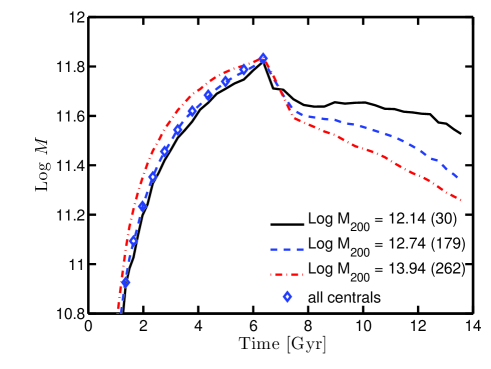
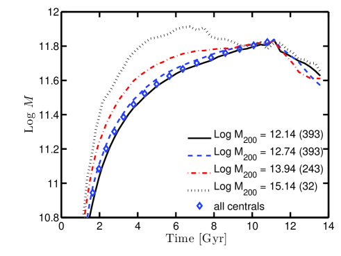
Figure 5: Main-progenitor histories of subhaloes with the same infall mass and redshift, split by their host mass at $\emph{z}=0$, $M_{\rm 200}$. Each panel includes histories for a given values of $\emph{z}_{\rm infall}$ and $M_{\rm infall}$. We track the main-progenitor histories starting $\emph{z}=0$, so only subhaloes which survive until $\emph{z}=0$ are included. Diamond symbols show the averaged main-progenitor histories for all central subhaloes which have the same mass at the infall redshift. Each $M_{\rm 200}$ bin includes values within 0.2 dex in Log$M_{\odot}$, where the number of main-progenitor histories used in each bin is given in parentheses. All values are taken from the full Millennium simulation. Time is in Gyr since the big-bang.

We first test this effect for the underlying dark-matter evolution, using subhaloes from the Millennium simulation. In Fig. 5 we show the main-progenitor histories of subhaloes with the same $M_{\rm infall}$ and $\emph{z}_{\rm infall}$. We split the average histories into different subsets of equal $M_{\rm 200}$ (the host of these subhaloes at $\emph{z}=0$). Also plotted in the same figure are the average histories of central subhaloes identified at the same $\emph{z}_{\rm infall}$. Indeed, merger-histories at early times are correlated to the $M_{\rm 200}$ mass at $\emph{z}=0$, especially if the infall redshift is low. This effect is very similar to the environmental effect mentioned above, where subhaloes that fall into more massive $M_{\rm 200}$ form earlier (i.e., the redshift which corresponds to half the current mass is higher).

In order to test the effect of $M_{\rm 200}$ on early formation histories of galaxies, we stop all modes of SF and merging for satellite galaxies in models $A1$ and $B1$. In all other aspects these models are the same as models $A0$ and $B0$. Consequently, in models $A1$ and $B1$, the stellar mass of satellite galaxies at $\emph{z}=0$ is identical to their mass at $\emph{z}_{\rm infall}$. The reader is referred again to Fig. 4, where the $m_{\rm star}-M_{\rm infall}$ relation is plotted for models $A1$ and $B1$. Not surprisingly, the stellar mass of satellite galaxies is already different at $\emph{z}_{\rm infall}$ from the stellar mass of central galaxies. This difference can reach 70 per cent in model $A1$ for the average value of $m_{\rm star}$, at $M_{\rm infall}\sim 3\times 10^{12}M_{\odot}$.

The effect of $M_{\rm 200}$ on $m_{\rm star}$ at early epochs can modify the CFs, and might contribute to the effect of shuffling discussed in section 3. The reason that there is no change in the CF due to shuffling in models $A1$ and $B1$ might be that the effect of environment is maximal in these models, which seems to cancel the contribution of other effects going in the opposite direction. We will discuss this issue further in section 5.

4.4 Stellar mass growth after infall

The amount of stellar mass gained by galaxies of type 1 & 2 after $\emph{z}_{\rm infall}$ can be seen in Fig. 4, when comparing the various models to models $A1$,$B1$. Models with slow gas stripping within satellite galaxies ($A0$, $A4$ & $B2$) show a significant increase of mass after infall, while models with fast stripping show only a minor change ($B0$ & $A2$). In models with slow stripping mechanism, more hot gas is available for cooling, and consequently more cold gas can reach the disk and form stars. Both observational and theoretical studies indicate that slow stripping is the preferred scenario for modeling the environmental evolution of galaxies within their host halo (McCarthy et al., 2008; Font et al., 2008; Khochfar & Ostriker, 2008; Weinmann et al., 2010).

In model $A4$ we use stripping of hot gas which is proportional to the dark-matter stripping. This scenario was found by Weinmann et al. (2010) to reproduce the fraction of passive satellite galaxies as a function of group mass and distance from the group center. In this case, the stripping rate will be correlated to the dark-matter evolution. From Fig. 5 it seems that the dark-matter evolution of subhaloes after $\emph{z}_{\rm infall}$ is affected by $M_{\rm 200}$, the group mass at $\emph{z}=0$. This is probably a natural consequence of the tidal interaction within the group. As a result of the above, the amount of $m_{\rm star}$ gained after infall should correlate with $M_{\rm 200}$ in this model. On the other hand, it may be expected that galaxies with higher $\emph{z}_{\rm infall}$ will have more time to increase their $m_{\rm star}$, so correlation with $\emph{z}_{\rm infall}$ is also expected.

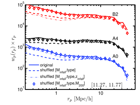
Figure 6: The CFs for various models using a range in $m_{\rm star}$ as indicated in units of Log$M_{\odot}$. For each model we run a few different shuffling tests, where the groups of shuffled galaxies are constrained to have the same set of properties: $M_{\rm infall}$ and galaxy type (dashed lines); $M_{\rm infall}$, galaxy type, and $\emph{z}_{\rm infall}$ (dashed-dotted lines); $M_{\rm infall}$, galaxy type, and $M_{\rm 200}$ (diamonds). An ABM model using two parameters for fixing the stellar mass of galaxies, namely $M_{\rm infall}$ and $M_{\rm 200}$, is shown to reproduce the CFs of the SAM galaxies.

5 ABM with an additional parameter

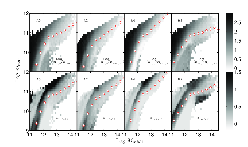
Figure 7: The behaviour of $M_{\rm 200}$ and $\emph{z}_{\rm infall}$ as a function of $M_{\rm infall}$ and $m_{\rm star}$ for satellite galaxies (type 1 & 2). Upper panels: median values of Log $M_{\rm 200}/M_{\rm infall}$; Lower panels: median values $\emph{z}_{\rm infall}$. Color coding is set to span 95 per cent of the population of $\emph{z}_{\rm infall}$ and $M_{\rm 200}/M_{\rm infall}$. Each panel shows results for one model as indicated. For the list of all models please see Table 1. Median values are computed for bins with more than 10 galaxies. Diamonds show the median $m_{\rm star}$ for all galaxies in the same $M_{\rm infall}$ bin.

In section 3 we saw that SAMs include additional clustering information which is not reproduced by a dependence on $M_{\rm infall}$ only. This was demonstrated by the different CF results when performing shuffling. We then learned that a single $m_{\rm star}-M_{\rm infall}$ relation cannot reproduce accurately the behaviour of satellite galaxies. It is not easy to disentangle the different reasons for the deviation in the $m_{\rm star}-M_{\rm infall}$ relation, and their affect on the CFs. This will require studying SAMs which include only one deviation per a model. For example, we would need to develop a SAM in which there is no redshift evolution in the mass relation, but satellite galaxies do increase their stellar mass function after infall. Here we choose to present a more modest test. Instead of modifying the SAMs, we will present a modification of ABMs which is able mimic the behaviour of SAMs better.

The target of this section is to present a more detailed version of ABMs which is relatively simple to use, and is able to fit the CF of SAMs. This is achieved by adding an additional parameter to ABMs, so the stellar mass of a galaxy is fixed not only by $M_{\rm infall}$ and the galaxy type, but also according to an additional ingredient. According to the previous section, there are two parameters which naturally affect the stellar mass of satellite galaxies: the infall redshift ($\emph{z}_{\rm infall}$), and the group mass at redshift zero ($M_{\rm 200}$). These parameters are correlated because of the hierarchical build-up of haloes (galaxies inside more massive groups tend to have a higher $\emph{z}_{\rm infall}$). Consequently, it is hard to separate the effect of each parameter on the models.

An important criterion for choosing the second parameter is the behaviour of the shuffled CFs. In order to check this issue, we present two additional shuffling tests. For each of the parameters tested ($p=\emph{z}_{\rm infall}$,$M_{\rm 200}$) we divide the catalog of galaxies into groups of the same $M_{\rm infall}$, type, and $p$ values as discussed in section 3. The location of galaxies are shuffled within these new groups. The resulting CFs are shown in Fig. 6. For all the models tested here, using the group mass, $M_{\rm 200}$, results in no change in the CF after shuffling. This means that SAMs have no additional clustering information except the dependence on $M_{\rm infall}$, $M_{\rm 200}$, and galaxy type. Consequently, ABMs that would use $M_{\rm 200}$ to fix the stellar mass in addition to $M_{\rm infall}$ would be able to reproduce the results of SAMs. Such models might have more freedom and could span more possible $m_{\rm star}-M_{\rm infall}$ relations.

Naively, one may expect that the main variation in the $m_{\rm star}-M_{\rm infall}$ relation should be due to the the additional dependence of satellite mass on $\emph{z}_{\rm infall}$. However, this parameter does not allow ABMs to better follow the CF of SAMs. In Fig. 6, adding $\emph{z}_{\rm infall}$ as a second parameter makes the CF of model $B2$ to deviate even more from the original CF. Adding $\emph{z}_{\rm infall}$ to model $A0$ improves the CF, but it does not reach the accuracy achieved by using $M_{\rm 200}$. The failure of $\emph{z}_{\rm infall}$ to improve ABMs is surprising, as it naturally affects the stellar mass of satellite galaxies. However, it seems that its correlation with stellar mass is weaker than the correlation between $M_{\rm 200}$ and stellar mass.

We have examined various statistical aspects of the effect of $M_{\rm 200}$ and $\emph{z}_{\rm infall}$ on $m_{\rm star}$ (per a given $M_{\rm infall}$). The main obstacle in presenting a clear-cut evidence for why $M_{\rm 200}$ works better than $\emph{z}_{\rm infall}$ is the different abundance of satellite galaxies as a function of $\emph{z}_{\rm infall}$ and $M_{\rm 200}$. For example, most satellite galaxies have $\emph{z}_{\rm infall}<1$ (see e.g. Gao et al., 2004), but have a different unique range in $M_{\rm 200}/M_{\rm infall}$. A clear comparison should take this number distribution into account. We therefore plot in Fig. 7 the median values of $M_{\rm 200}$ and $\emph{z}_{\rm infall}$ per each bin in $m_{\rm star}$ and $M_{\rm infall}$. When comparing $M_{\rm 200}$ against $\emph{z}_{\rm infall}$, the number of galaxies per each bin remains the same. However, we note that most of the galaxies are concentrated around the median $m_{\rm star}$ values (diamond symbols).

Fig. 7 shows the reason for the success of $M_{\rm 200}$ as a second parameter. The dependence of $m_{\rm star}$ on $M_{\rm 200}$ (for a given $M_{\rm infall}$) is roughly monotonic and smooth. For a given $M_{\rm infall}$, the values of $M_{\rm 200}$ span nicely the scatter in $m_{\rm star}$. A different behaviour is seen for $\emph{z}_{\rm infall}$. The relation between $m_{\rm star}$ and $\emph{z}_{\rm infall}$ for a given $M_{\rm infall}$ is not monotonic. This means that the dependence of $m_{\rm star}$ on $\emph{z}_{\rm infall}$ is in general not unique, so very different $m_{\rm star}$ correspond to the same $\emph{z}_{\rm infall}$. For example, consider model $B2$ (lower-right panel): shuffling galaxies with the same $M_{\rm infall}\sim 10^{13}$ and $\emph{z}_{\rm infall}\sim 1$ will result in swapping galaxies between very different stellar masses (the dark regions). As can be seen from the upper panel, the swapped galaxies live inside different fof groups, so this shuffling will affect the CF significantly. This is probably the reason why $\emph{z}_{\rm infall}$ does not improve the shuffled CF in model $B2$. We note that the range in $m_{\rm star}$ used for testing the shuffled CFs in Fig. 6 corresponds to $M_{\rm infall}\gtrsim 10^{12}M_{\odot}$. As the number of subhaloes of a given $M_{\rm infall}$ decreases quickly with increasing $M_{\rm infall}$; the CF in this mass range is mostly affected by $M_{\rm infall}\sim 10^{12}M_{\odot}$.

6 Summary and discussion

In this work we have studied the relation between the mass of subhaloes ($M_{\rm infall}$) and the stellar mass of galaxies. A simple model for this relation is crucial for summarizing the basic concepts of galaxy formation physics. It can then be used to model the correlation function of galaxies, their stellar mass function, star-formation rates, and merging processes. The abundance matching approach (ABM) is aiming at constraining this mass relation directly, without the need to rely on the assumptions of a specific model. This constraint is important because other theoretical methodologies depend strongly on the detailed physics assumed, and are usually not able to match the observational constraints accurately. It is therefore necessary to study the assumptions made by the ABM approach, and their effect on the mass relation above.

In this paper we have tested the basic assumptions of ABM models using a set of Semi-Analytical Models (SAMs) developed by Neistein & Weinmann (2010). We examined the relation between stellar mass and $M_{\rm infall}$ within the SAMs at different redshifts, and for satellite versus central galaxies. It was shown that a single $m_{\rm star}-M_{\rm infall}$ relation is not able to capture accurately the full complexity of SAMs, due to complex behaviour of satellite galaxies. First, the stellar mass of these galaxies behaves differently at early times due to an environmental effect acting on their host haloes (the ‘assembly bias’; Gao et al., 2005; Harker et al., 2006). Satellite galaxies falling into more massive groups have different dark-matter merger-histories, and are more massive even before falling into their group. Second, the mass of satellite galaxies depends on the infall redshift ($\emph{z}_{\rm infall}$, defined as the time they became satellites). This is because they roughly follow the global behaviour of central galaxies. Third, satellite galaxies acquire a significant amount of stellar mass after $\emph{z}_{\rm infall}$, especially if the model assumes slow gas stripping mechanisms. This growth can reach a factor of $\sim 2$ in stellar mass, for galaxies with $\emph{z}_{\rm infall}=1$.

We have used the shuffling technique, where the location of all model galaxies that have the same $M_{\rm infall}$ and galaxy type (central/satellite) are swapped randomly. Assuming that the stellar mass of galaxies depends only on the host subhalo mass ($M_{\rm infall}$), is equivalent to using a shuffled sample of galaxies. In order to check the effect of this assumption on the clustering properties of galaxies, we compared the auto correlation functions (CFs) of the original SAMs against the shuffled catalogs. We found that shuffled catalogs of galaxies can have different CFs, depending on the specific model being tested. The shuffled CFs are very different if we assume the same $m_{\rm star}-M_{\rm infall}$ relation for satellite and central galaxies, reaching a factor of $\sim 4$ at scales below 1 Mpc. However, even when using a different $m_{\rm star}-M_{\rm infall}$ relation for central and satellite galaxies, this difference can reach a factor of 2 in the CF of the most massive galaxies.

The results shown here are based on a few specific SAMs and might not reflect the ‘true’ physical Universe. It might be that the assumptions adopted by ABM models are correct, and SAMs introduce more complexity than what is needed. However, it might be that the ‘true’ model includes a different set of assumptions, or is more extreme in violating the assumptions tested here. A different limitation of this work is that the results of the auto-correlation functions obtained here are based on the Millennium simulation. This simulation assumes $\sigma_{8}=0.9$, which is higher than the latest favorable estimates. As a result, the relation between the model CFs and the observed data is of less interest to this study. We did not aim at providing a model which reproduce the observed values of both the stellar mass function and the CFs.

We have checked two additional parameters which could be adopted by future ABM models in order to better reproduce the results of SAMs. For the SAMs used here, assuming that the stellar mass depends on $M_{\rm infall},\,M_{\rm 200}$ and galaxy type is enough to reproduce the CF of galaxies ($M_{\rm 200}$ is the fof group mass at redshift zero). The other natural parameter, $\emph{z}_{\rm infall}$ does not provide a good match to the clustering of SAMs probably because it is less correlated with the stellar mass. Using $M_{\rm 200}$ as a second parameter makes ABM models more similar to HODs, in which all the properties of galaxies are fixed by the group mass.

Our results may be relevant for interpreting the observed environmental dependencies of galaxies. While various results stress the importance of late evolution on the properties of satellite galaxies (e.g. Kauffmann et al., 2004), we find evidence for the influence of early evolution. At a fixed $M_{\rm infall}$, galaxies ending up in massive clusters undergo a more rapid growth of their dark matter halo at early times, which may influence their observed properties at late times, like their morphology or star formation rate.

Studies like van den Bosch et al. (2008) and Weinmann et al. (2009) investigate the impact of environment by comparing satellite and central galaxies at fixed stellar mass today. van den Bosch et al. (2008) argue that this is reasonable, as most satellites fall in late, and thus no large difference in the evolution of stellar mass between central and satellite galaxies since this time is expected. However, as we have shown here, the progenitors of today’s satellites and the progenitors of today’s centrals may be different already at redshifts before the time of infall. Depending on the exact nature and magnitude of this effect, it may complicate the direct comparison between central and satellite galaxies. In a future work we intend to study the differences in stellar mass between satellite and central galaxies in more detail, making use of the two parameter ABM approach suggested in this work.

Appendix

In this Appendix we provide more CF plots for models $B0$ and $A4$ (Figs. 8, 9). We also plot the stellar mass function for all the models used in this work against the observational data in Fig. 10.

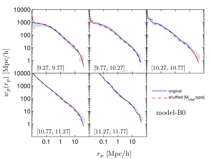
Figure 8: The projected auto-correlation functions derived for model $B0$. Each panel corresponds to galaxies with stellar masses as indicated, in units of Log$M_{\odot}$. Solid lines show the results of the original model, dashed lines are plotted using shuffling within [$M_{\rm infall}$,type]. The observational data are using SDSS DR7 with the same technique as in Li et al. (2006), and are shown as error bars.

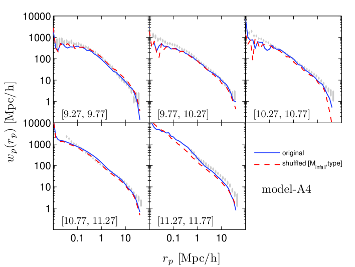
Figure 9: Similar to Fig. 8, but for model $A4$.

Figure 10: Stellar mass functions of galaxies at various redshifts, for our different models as indicated in the top left panel and as summarized in table 1. The observational data is plotted with gray symbols. At all redshifts higher than zero we convolve the model stellar masses with a Gaussian error distribution, with standard deviation of 0.25 dex. At $\emph{z}=0$ we use observations by Li & White (2009, circles), Baldry et al. (2008, crosses), Panter et al. (2007, pluses). Note that other observational studies predict a slightly different function (e.g. Bernardi et al., 2010). At high-z we use the following observations: Bundy et al. (2006, $\emph{z}=0.75-1$, circles), Borch et al. (2006, $\emph{z}=0.8-1$, crosses), Pérez-González et al. (2008, $\emph{z}=0.8-1$, $\emph{z}=1.6-2$, $\emph{z}=2.5-3$, plus signs), Fontana et al. (2006, $\emph{z}=0.8-1$, $\emph{z}=1.6-2$, $\emph{z}=2-3$, stars), Drory et al. (2004, $\emph{z}=0.8-1$, upward-pointing triangles), Drory et al. (2005, $\emph{z}=0.75-1.25$, $\emph{z}=1.75-2.25$, $z=2.25-3$, diamonds and squares), Marchesini et al. (2009, $\emph{z}=1.3-2$, $\emph{z}=2-3$, right-pointing triangles). Model stellar mass functions are plotted at $\emph{z}=0$, 1, 1.5, 2.5 according to the label on each panel. We treat the specific IMF chosen in each measurement as part of the observational ‘uncertainty’ and do not convert them into the same IMF.

References

- Baldry et al. (2008) Baldry I. K., Glazebrook K., Driver S. P., 2008, MNRAS, 388, 945
- Behroozi et al. (2010) Behroozi P. S., Conroy C., Wechsler R. H., 2010, ApJ, 717, 379
- Berlind & Weinberg (2002) Berlind A. A., Weinberg D. H., 2002, ApJ, 575, 587
- Bernardi et al. (2010) Bernardi M., Shankar F., Hyde J. B., Mei S., Marulli F., Sheth R. K., 2010, MNRAS, 404, 2087
- Binney & Tremaine (1987) Binney J., Tremaine S., 1987, Galactic dynamics
- Bode et al. (2001) Bode P., Ostriker J. P., Turok N., 2001, ApJ, 556, 93
- Borch et al. (2006) Borch A., et al., 2006, A&A, 453, 869
- Bundy et al. (2006) Bundy K., et al., 2006, ApJ, 651, 120
- Conroy et al. (2007) Conroy C., Prada F., Newman J. A., Croton D., Coil A. L., Conselice C. J., Cooper M. C., Davis M., Faber S. M., Gerke B. F., Guhathakurta P., Klypin A., Koo D. C., Yan R., 2007, ApJ, 654, 153
- Conroy & Wechsler (2009) Conroy C., Wechsler R. H., 2009, ApJ, 696, 620
- Conroy et al. (2006) Conroy C., Wechsler R. H., Kravtsov A. V., 2006, ApJ, 647, 201
- Cox et al. (2008) Cox T. J., Jonsson P., Somerville R. S., Primack J. R., Dekel A., 2008, MNRAS, 384, 386
- Croton et al. (2006) Croton D. J., et al., 2006, MNRAS, 365, 11
- Croton et al. (2007) Croton D. J., Gao L., White S. D. M., 2007, MNRAS, 374, 1303
- Davis et al. (1985) Davis M., Efstathiou G., Frenk C. S., White S. D. M., 1985, ApJ, 292, 371
- De Lucia & Blaizot (2007) De Lucia G., Blaizot J., 2007, MNRAS, 375, 2
- Drory et al. (2004) Drory N., Bender R., Feulner G., Hopp U., Maraston C., Snigula J., Hill G. J., 2004, ApJ, 608, 742
- Drory et al. (2005) Drory N., Salvato M., Gabasch A., Bender R., Hopp U., Feulner G., Pannella M., 2005, ApJ, 619, L131
- Font et al. (2008) Font A. S., Bower R. G., McCarthy I. G., Benson A. J., Frenk C. S., Helly J. C., Lacey C. G., Baugh C. M., Cole S., 2008, MNRAS, 389, 1619
- Fontana et al. (2006) Fontana A., Salimbeni S., Grazian A., Giallongo E., Pentericci L., Nonino M., Fontanot F., Menci N., Monaco P., Cristiani S., Vanzella E., de Santis C., Gallozzi S., 2006, A&A, 459, 745
- Gao et al. (2005) Gao L., Springel V., White S. D. M., 2005, MNRAS, 363, L66
- Gao et al. (2004) Gao L., White S. D. M., Jenkins A., Stoehr F., Springel V., 2004, MNRAS, 355, 819
- Guo et al. (2010) Guo Q., White S., Boylan-Kolchin M., De Lucia G., Kauffmann G., Lemson G., Li C., Springel V., Weinmann S., 2010, ArXiv e-prints: 1006.0106
- Guo et al. (2010) Guo Q., White S., Li C., Boylan-Kolchin M., 2010, MNRAS, 404, 1111
- Harker et al. (2006) Harker G., Cole S., Helly J., Frenk C., Jenkins A., 2006, MNRAS, 367, 1039
- Kauffmann et al. (2004) Kauffmann G., White S. D. M., Heckman T. M., Ménard B., Brinchmann J., Charlot S., Tremonti C., Brinkmann J., 2004, MNRAS, 353, 713
- Khochfar & Ostriker (2008) Khochfar S., Ostriker J. P., 2008, ApJ, 680, 54
- Kravtsov et al. (2004) Kravtsov A. V., Berlind A. A., Wechsler R. H., Klypin A. A., Gottlöber S., Allgood B., Primack J. R., 2004, ApJ, 609, 35
- Li et al. (2006) Li C., Kauffmann G., Jing Y. P., White S. D. M., Börner G., Cheng F. Z., 2006, MNRAS, 368, 21
- Li & White (2009) Li C., White S. D. M., 2009, MNRAS, 398, 2177
- Macciò & Fontanot (2010) Macciò A. V., Fontanot F., 2010, MNRAS, 404, L16
- Mandelbaum et al. (2006) Mandelbaum R., Seljak U., Kauffmann G., Hirata C. M., Brinkmann J., 2006, MNRAS, 368, 715
- Marchesini et al. (2009) Marchesini D., van Dokkum P. G., Förster Schreiber N. M., Franx M., Labbé I., Wuyts S., 2009, ApJ, 701, 1765
- McCarthy et al. (2008) McCarthy I. G., Frenk C. S., Font A. S., Lacey C. G., Bower R. G., Mitchell N. L., Balogh M. L., Theuns T., 2008, MNRAS, 383, 593
- Mihos & Hernquist (1994) Mihos J. C., Hernquist L., 1994, ApJ, 431, L9
- Moster et al. (2010) Moster B. P., Somerville R. S., Maulbetsch C., van den Bosch F. C., Macciò A. V., Naab T., Oser L., 2010, ApJ, 710, 903
- Neistein & Weinmann (2010) Neistein E., Weinmann S. M., 2010, MNRAS, 405, 2717 (NW10)
- Panter et al. (2007) Panter B., Jimenez R., Heavens A. F., Charlot S., 2007, MNRAS, 378, 1550
- Pérez-González et al. (2008) Pérez-González P. G., Rieke G. H., Villar V., Barro G., Blaylock M., Egami E., Gallego J., Gil de Paz A., Pascual S., Zamorano J., Donley J. L., 2008, ApJ, 675, 234
- Sawala et al. (2010) Sawala T., Guo Q., Scannapieco C., Jenkins A., White S. D. M., 2010, ArXiv e-prints, 1003.0671
- Shankar et al. (2006) Shankar F., Lapi A., Salucci P., De Zotti G., Danese L., 2006, ApJ, 643, 14
- Somerville et al. (2001) Somerville R. S., Primack J. R., Faber S. M., 2001, MNRAS, 320, 504
- Springel et al. (2005) Springel V., White S. D. M., Jenkins A., Frenk C. S., Yoshida N., Gao L., Navarro J., Thacker R., Croton D., Helly J., Peacock J. A., Cole S., Thomas P., Couchman H., Evrard A., Colberg J., Pearce F., 2005, Nature, 435, 629
- Springel et al. (2001) Springel V., White S. D. M., Tormen G., Kauffmann G., 2001, MNRAS, 328, 726
- Tinker et al. (2005) Tinker J. L., Weinberg D. H., Zheng Z., Zehavi I., 2005, ApJ, 631, 41
- Vale & Ostriker (2004) Vale A., Ostriker J. P., 2004, MNRAS, 353, 189
- van den Bosch et al. (2008) van den Bosch F. C., Aquino D., Yang X., Mo H. J., Pasquali A., McIntosh D. H., Weinmann S. M., Kang X., 2008, MNRAS, 387, 79
- Wang et al. (2006) Wang L., Li C., Kauffmann G., De Lucia G., 2006, MNRAS, 371, 537
- Wechsler et al. (2006) Wechsler R. H., Zentner A. R., Bullock J. S., Kravtsov A. V., Allgood B., 2006, ApJ, 652, 71
- Weinmann et al. (2009) Weinmann S. M., Kauffmann G., van den Bosch F. C., Pasquali A., McIntosh D. H., Mo H., Yang X., Guo Y., 2009, MNRAS, 394, 1213
- Weinmann et al. (2010) Weinmann S. M., Kauffmann G., von der Linden A., De Lucia G., 2010, MNRAS, 406, 2249
- Yang et al. (2009) Yang X., Mo H. J., van den Bosch F. C., 2009, ApJ, 695, 900
- Zehavi et al. (2005) Zehavi I., et al., 2005, ApJ, 630, 1