$N$-Dark-Dark Solitons in the Generally Coupled Nonlinear Schrödinger Equations

Abstract

$N$-dark-dark solitons in the generally coupled integrable NLS equations are derived by the KP-hierarchy reduction method. These solitons exist when nonlinearities are all defocusing, or both focusing and defocusing nonlinearities are mixed. When these solitons collide with each other, energies in both components of the solitons completely transmit through. This behavior contrasts collisions of bright-bright solitons in similar systems, where polarization rotation and soliton reflection can take place. It is also shown that in the mixed-nonlinearity case, two dark-dark solitons can form a stationary bound state.

Keywords: Coupled nonlinear Schrödinger equations, KP hierarchy, dark-dark solitons, $\tau$ function.

1 Introduction

In studies of nonlinear wave dynamics in physical systems, nonlinear Schrödinger (NLS)-type equations play a prominent role. It is known that a weakly nonlinear one-dimensional wave packet in a generic physical system is governed by the NLS equation [1]. Hence this equation appears frequently in nonlinear optics and water waves [2, 3, 4]. Recently, it has been shown that the nonlinear interaction of atoms in Bose-Einstein condensates is governed by a NLS-type equation as well (called Gross-Pitaevskii equation in the literature) [5]. In these physical systems, the nonlinearity can be focusing or defocusing (i.e., the nonlinear coefficient can be positive or negative), depending on the physical situations [4] or the types of atoms in Bose-Einstein condensates [5]. When two wave packets in a physical system or two types of atoms in Bose-Einstein condensates interact with each other, their interaction then is governed by two coupled NLS equations [2, 3, 6, 7, 8, 9, 10, 11]. The single NLS equation is exactly integrable [12]. It admits bright solitons in the focusing case, and dark solitons in the defocusing case. Its bright $N$-soliton solutions were given in [12], and its dark $N$-soliton solutions can be found in [13]. The coupled NLS equations are also integrable when the nonlinear coefficients have the same magnitudes [14, 15, 16]. In these integrable cases, if all nonlinear terms are of focusing type (i.e., the nonlinear coefficients are all positive), the coupled NLS equations are the focusing Manakov model which admits bright-bright solitons [14]. If all nonlinear terms are of defocusing type (i.e., the nonlinear coefficients are all negative), the coupled NLS equations are the defocusing Manakov model which admits bright-dark and dark-dark solitons [17, 18, 19]. If the focusing and defocusing nonlinearities are mixed (i.e., the nonlinear coefficients have opposite signs), these coupled NLS equations admit bright-bright solitons [16, 20] and bright-dark solitons [21]. Existence of dark-dark solitons in this mixed case has not been investigated yet.

Soliton interaction in these integrable generally coupled NLS equations is a fascinating subject. In the focusing Manakov model, an interesting phenomenon is that bright solitons change their polarizations (i.e. relative energy distributions among the two components) after collision [14]. In the coupled NLS equations with mixed nonlinearities, energy can also transfer from one soliton to another after collision [20]. In addition, solitons can be reflected off by each other as well [16]. In the defocusing Manakov model, two bright-dark solitons can form a stationary bound state, a phenomenon which does not occur for scalar bright or dark solitons [17]. All these interesting interaction behaviors can be described by multi-soliton solutions in the underlying integrable system. In the focusing Manakov model, $N$-bright-bright solitons were derived in [14] by the inverse scattering transform method. In the mixed-nonlinearity model, two- and three-bright-bright solitons and two-bright-dark solitons were derived in [20, 21] by the Hirota method, and $N$-bright-bright solitons were derived in [16] by the Riemann-Hilbert method. In the defocusing Manakov model, $N$-bright-dark solitons were derived in [17], and degenerate two-dark-dark solitons were derived in [18], both by the Hirota method.

So far, progress on dark-dark solitons in the integrable generally coupled NLS equations is very limited. While dark-dark solitons in the defocusing Manakov model were derived in [18], we will show that their two- and higher-dark-dark solitons are actually degenerate and reducible to scalar dark solitons. In [19], the inverse scattering transform method was developed for dark solitons in the defocusing Manakov model. But, as we will show in this paper, their analysis can not yield general dark-dark solitons either due to their choices of the boundary conditions. To date, general multi-dark-dark solitons in the coupled NLS equations have never been reported yet (to our knowledge). As we will see, these general multi-dark-dark solitons are not easy to obtain due to non-trivial parameter constraints which must be met.

In this paper, we comprehensively analyze dark-dark solitons and their dynamics in the generally coupled integrable NLS equations. First, we show that these coupled NLS equations can be obtained as a reduction of the Kadomtsev-Petviashvili (KP) hierarchy. Then using $\tau$-function solutions of the KP hierarchy, we derive the general $N$-dark-dark solitons in terms of Gram determinants. These dark-dark solitons exist in both the defocusing Manakov model and the mixed-nonlinearity model. Recalling that bright-bright solitons exist in the mixed-nonlinearity model as well [16, 18], we see that the coupled NLS equations with mixed nonlinearities are the rare integrable systems which admit both bright-bright and dark-dark solitons. The dark-dark solitons obtained previously in [18, 19] for the defocusing Manakov model are only degenerate cases of our general solutions. Next, we analyze properties of these soliton solutions. For single dark-dark solitons, we show that the degrees of “darkness” in their two components are different in general. When two dark-dark solitons collide with each other, we show that energies in the two components of each soliton completely transmit through. This contrasts collisions of bright-bright solitons in these same equations, where polarization rotation, power transfer and soliton reflection can occur [14, 16, 20]. Thus dark-dark solitons are much more robust than bright-bright solitons with regard to collision. In the case of mixed focusing and defocusing nonlinearities, an interesting phenomenon is that two dark-dark solitons can form a stationary bound state. This is the first report of dark-dark-soliton bound states in integrable systems. However, three or more dark-dark solitons can not form bound states, as we will show in this paper.

We should mention that this KP-hierarchy reduction for deriving soliton solutions in integrable systems was first developed by the Kyoto school in the 1970s [22]. So far, this method has been applied to derive bright solitons in many equations such as NLS, modified KdV, Davey-Stewartson equations [23, 24, 25]. This method has also been applied to derive $N$-dark solitons in the defocusing NLS equation [25]. But this reduction for dark-dark solitons in the generally coupled NLS equations is more subtle and has never been done before. In this paper, we will derive general $N$-dark-dark solitons by this KP-hierarchy reduction and the grace of deep use of determinant expressions. Compared to the inverse scattering transform method [19] and the Hirota method [18], our treatment is much more clean, and the solution formulae much more elegant and general. Thus, the KP-reduction method has a distinct advantage in derivations of dark-soliton solutions.

2 The $N$-dark-dark solitons

The generally coupled integrable NLS equations we investigate in this paper are

$$\begin{array}[]{ll}iu_{t}=u_{xx}+(\delta|u|^{2}+\epsilon|v|^{2})u,\\ iv_{t}=v_{xx}+(\delta|u|^{2}+\epsilon|v|^{2})v,\end{array}$$ (1)

where $\delta$ and $\epsilon$ are real coefficients. This system is integrable [14, 15, 16]. Through $u$ and $v$ scalings, the nonlinear coefficients $\delta$ and $\epsilon$ can be normalized to be $\pm 1$ without loss of generality. When $\epsilon=\delta=1$, this system is the focusing Manakov model which supports bright-bright solitons [14]. When $\epsilon=\delta=-1$, this system is the defocusing Manakov model which supports bright-dark and dark-dark solitons [17, 18, 19]. When $\epsilon$ and $\delta$ have opposite signs, the system exhibits mixed focusing and defocusing nonlinearities. In this case, these equations support bright-bright solitons [16, 20], bright-dark solitons [21], and dark-dark solitons (as we will see below).

In this section, we derive the general formulae for $N$-dark-dark solitons in the integrable coupled NLS system (1). The basic idea is to treat Eq. (1) as a reduction of the KP hierarchy. Then dark solitons in Eq. (1) can be obtained from solutions of the KP hierarchy under this reduction. For this purpose, let us first review Gram-type solutions for equations in the KP hierarchy [26, 27, 28].

Lemma 1

Consider the following equations in the KP hierarchy [29, 30]

$$\begin{array}[]{ll}(\frac{1}{2}D_{x}D_{r}-1)\tau(k)\cdot\tau(k)=-\tau(k+1)\tau(k-1),\\ (D_{x}^{2}-D_{y}+2aD_{x})\tau(k+1)\cdot\tau(k)=0,\end{array}$$ (2)

where $D$ is the Hirota derivative defined by

$$D_{x}^{m}D_{y}^{n}\hskip 0.85355ptf(x,y)\cdot g(x,y)\equiv\left(\frac{\partial}{\partial x}-\frac{\partial}{\partial x^{\prime}}\right)^{m}\left(\frac{\partial}{\partial y}-\frac{\partial}{\partial y^{\prime}}\right)^{n}f(x,y)\hskip 1.70709ptg(x^{\prime},y^{\prime})|_{x=x^{\prime},\hskip 2.27626pty=y^{\prime}}\hskip 2.27626pt,$$ (3)

$a$ is a complex constant, $k$ is an integer, and $\tau(k)$ is a function of three independent variables $(x,y,r)$. The Gram determinant solution $\tau(k)$ of the above equations is given by

$$\tau(k)=\mathrm{det}_{1\leq i,j\leq N}\Big{(}m_{ij}(k)\Big{)}=\Big{|}m_{ij}(k)\Big{|}_{1\leq i,j\leq N},$$

where the matrix element $m_{ij}(k)$ satisfies

$$\begin{array}[]{ll}\partial_{x}m_{ij}(k)=\varphi_{i}(k)\psi_{j}(k),\\ \partial_{y}m_{ij}(k)=(\partial_{x}\varphi_{i}(k))\psi_{j}(k)-\varphi_{i}(k)(\partial_{x}\psi_{j}(k)),\\ \partial_{r}m_{ij}(k)=-\varphi_{i}(k-1)\psi_{j}(k+1),\\ m_{ij}(k+1)=m_{ij}(k)+\varphi_{i}(k)\psi_{j}(k+1),\end{array}$$ (4)

and $\varphi_{i}(k)$ and $\psi_{j}(k)$ are arbitrary functions satisfying

$$\begin{array}[]{ll}\partial_{y}\varphi_{i}(k)=\partial_{x}^{2}\varphi_{i}(k),\\ \varphi_{i}(k+1)=(\partial_{x}-a)\varphi_{i}(k),\\ \partial_{y}\psi_{j}(k)=-\partial_{x}^{2}\psi_{j}(k),\\ \psi_{j}(k-1)=-(\partial_{x}+a)\psi_{j}(k).\end{array}$$ (5)

Before proving this lemma, several remarks are in order. The first equation in (2) is the bilinear equation for the two-dimensional Toda lattice (see p.984 of [29] and p.4130 of [30]), and the second equation in (2) is the lowest-degree bilinear equation in the 1st modified KP hierarchy (see p.996 of [29]). Since the two-dimensional Toda lattice hierarchy and modified KP hierarchies are closely related to the (single-component) KP hierarchy, all these hierarchies will be called the KP hierarchy in this paper. Regarding the parameter $a$ in the second equation in (2), it corresponds to the wave-number shift $k_{0}$ in [29] [see Eq. (10.3) there]. The bilinear equation with this parameter was not explicitly written down in [29], but can be found in [30] [see Eq. (N-3) there]. This parameter can be formally removed by the Galilean transformation for $y$ in (2). But for our purpose, it proves to be important to keep this parameter, as it will pave the way for the introduction of another similar parameter $b$ in Lemma 2 later. In that case, $a$ and $b$ can not be removed simultaneously by the Galilean transformation, and they are essential for the construction of non-degenerate dark-dark solitons in the generally coupled NLS system (1).

Proof of Lemma 1. By using (4) and (5), we can verify that the derivatives and shifts of the $\tau$ function are expressed by the bordered determinants as follows

$$\begin{array}[]{ll}\partial_{x}\tau(k)=\left|\begin{array}[]{cc}m_{ij}(k)&\varphi_{i}(k)\cr-\psi_{j}(k)&0\end{array}\right|,\\ \partial_{x}^{2}\tau(k)=\left|\begin{array}[]{cc}m_{ij}(k)&\partial_{x}\varphi_{i}(k)\cr-\psi_{j}(k)&0\end{array}\right|+\left|\begin{array}[]{cc}m_{ij}(k)&\varphi_{i}(k)\cr-\partial_{x}\psi_{j}(k)&0\end{array}\right|,\\ \partial_{y}\tau(k)=\left|\begin{array}[]{cc}m_{ij}(k)&\partial_{x}\varphi_{i}(k)\cr-\psi_{j}(k)&0\end{array}\right|-\left|\begin{array}[]{cc}m_{ij}(k)&\varphi_{i}(k)\cr-\partial_{x}\psi_{j}(k)&0\end{array}\right|,\\ \partial_{r}\tau(k)=\left|\begin{array}[]{cc}m_{ij}(k)&\varphi_{i}(k-1)\cr\psi_{j}(k+1)&0\end{array}\right|,\\ (\partial_{x}\partial_{r}-1)\tau(k)=\left|\begin{array}[]{ccc}m_{ij}(k)&\varphi_{i}(k-1)&\varphi_{i}(k)\cr\psi_{j}(k+1)&0&-1\cr-\psi_{j}(k)&-1&0\end{array}\right|,\\ \tau(k+1)=\left|\begin{array}[]{cc}m_{ij}(k)&\varphi_{i}(k)\cr-\psi_{j}(k+1)&1\end{array}\right|,\\ \tau(k-1)=\left|\begin{array}[]{cc}m_{ij}(k)&\varphi_{i}(k-1)\cr\psi_{j}(k)&1\end{array}\right|,\\ (\partial_{x}+a)\tau(k+1)=\left|\begin{array}[]{cc}m_{ij}(k)&\partial_{x}\varphi_{i}(k)\cr-\psi_{j}(k+1)&a\end{array}\right|,\\ (\partial_{x}+a)^{2}\tau(k+1)=\left|\begin{array}[]{cc}m_{ij}(k)&\partial_{x}^{2}\varphi_{i}(k)\cr-\psi_{j}(k+1)&a^{2}\end{array}\right|+\left|\begin{array}[]{ccc}m_{ij}(k)&\partial_{x}\varphi_{i}(k)&\varphi_{i}(k)\cr-\psi_{j}(k+1)&a&1\cr-\psi_{j}(k)&0&0\end{array}\right|,\\ (\partial_{y}+a^{2})\tau(k+1)=\left|\begin{array}[]{cc}m_{ij}(k)&\partial_{x}^{2}\varphi_{i}(k)\cr-\psi_{j}(k+1)&a^{2}\end{array}\right|-\left|\begin{array}[]{ccc}m_{ij}(k)&\partial_{x}\varphi_{i}(k)&\varphi_{i}(k)\cr-\psi_{j}(k+1)&a&1\cr-\psi_{j}(k)&0&0\end{array}\right|.\end{array}$$

Here the bordered determinants are defined as

$$\left|\begin{array}[]{cc}m_{ij}&\varphi_{i}\cr-\psi_{j}&0\end{array}\right|\equiv\left|\begin{array}[]{ccccc}m_{11}&m_{12}&\cdots&m_{1N}&\varphi_{1}\\ m_{21}&m_{22}&\cdots&m_{2N}&\varphi_{2}\\ \vdots&\vdots&\vdots&\vdots&\vdots\\ m_{N1}&m_{N2}&\cdots&m_{NN}&\varphi_{N}\\ -\psi_{1}&-\psi_{2}&\cdots&-\psi_{N}&0\end{array}\right|,$$

and so on. By using the Jacobi formula of determinants [26], we obtain the bilinear equations (2) from the above expressions. $\Box$

Using Lemma 1, we can obtain solutions to a larger class of equations in the KP hierarchy below.

Lemma 2

Consider the following equations in the KP hierarchy,

$$\begin{array}[]{ll}(\frac{1}{2}D_{x}D_{r}-1)\tau(k,l)\cdot\tau(k,l)=-\tau(k+1,l)\tau(k-1,l),\\ (D_{x}^{2}-D_{y}+2aD_{x})\tau(k+1,l)\cdot\tau(k,l)=0,\\ (\frac{1}{2}D_{x}D_{s}-1)\tau(k,l)\cdot\tau(k,l)=-\tau(k,l+1)\tau(k,l-1),\\ (D_{x}^{2}-D_{y}+2bD_{x})\tau(k,l+1)\cdot\tau(k,l)=0,\end{array}$$ (6)

where $a,b$ are complex constants, $k,l$ are integers, and $\tau(k,l)$ is a function of four independent variables $(x,y,r,s)$. The solution $\tau(k,l)$ to these equations is given by the Gram determinant

$$\tau(k,l)=\mathrm{det}_{1\leq i,j\leq N}\Big{(}m_{ij}(k,l)\Big{)}=\Big{|}m_{ij}(k,l)\Big{|}_{1\leq i,j\leq N},$$ (7)

where the matrix element $m_{ij}(k,l)$ is defined by

$$\begin{array}[]{ll}m_{ij}(k,l)=c_{ij}+\frac{1}{p_{i}+q_{j}}\varphi_{i}(k,l)\psi_{j}(k,l),\\ \varphi_{i}(k,l)=(p_{i}-a)^{k}(p_{i}-b)^{l}e^{\xi_{i}},\\ \psi_{j}(k,l)=(-\frac{1}{q_{j}+a})^{k}(-\frac{1}{q_{j}+b})^{l}e^{\eta_{j}},\end{array}$$ (8)

with

$$\begin{array}[]{ll}\xi_{i}=p_{i}x+p_{i}^{2}y+\frac{1}{p_{i}-a}r+\frac{1}{p_{i}-b}s+\xi_{i0},\\ \eta_{j}=q_{j}x-q_{j}^{2}y+\frac{1}{q_{j}+a}r+\frac{1}{q_{j}+b}s+\eta_{j0},\end{array}$$ (9)

and $c_{ij}$, $p_{i}$, $q_{j}$, $\xi_{i0}$, $\eta_{j0}$ are complex constants.

It is noted that the system (6) is an expansion of the previous system (2) by adding a new pair of independent variables $(s,l)$ to the previous pair $(r,k)$.

Proof. It is easy to see that functions $m_{ij}(k,l)$, $\varphi_{i}(k,l)$ and $\psi_{j}(k,l)$ satisfy the following differential and difference rules,

$$\begin{array}[]{ll}\partial_{x}m_{ij}(k,l)=\varphi_{i}(k,l)\psi_{j}(k,l),\\ \partial_{y}m_{ij}(k,l)=(\partial_{x}\varphi_{i}(k,l))\psi_{j}(k,l)-\varphi_{i}(k,l)(\partial_{x}\psi_{j}(k,l)),\\ \partial_{r}m_{ij}(k,l)=-\varphi_{i}(k-1,l)\psi_{j}(k+1,l),\\ m_{ij}(k+1,l)=m_{ij}(k,l)+\varphi_{i}(k,l)\psi_{j}(k+1,l),\\ \partial_{y}\varphi_{i}(k,l)=\partial_{x}^{2}\varphi_{i}(k,l),\\ \varphi_{i}(k+1,l)=(\partial_{x}-a)\varphi_{i}(k,l),\\ \partial_{y}\psi_{j}(k,l)=-\partial_{x}^{2}\psi_{j}(k,l),\\ \psi_{j}(k-1,l)=-(\partial_{x}+a)\psi_{j}(k,l).\end{array}$$ (10)

Then from Lemma 1, we can verify the first two bilinear equations in (6). The other two equations in (6) can be obtained directly by replacing $a$, $k$, $r$ as $b$, $l$, $s$ in Eq. (2) of Lemma 1. $\Box$

Next, we perform a reduction to the bilinear system (6) in the KP hierarchy. Solutions to the reduced bilinear equations are given below.

Theorem 1

Assume that $f$ is a real function of real $x$ and $t,$ and $g,h$ are complex functions of real $x$ and $t,$ then the following bilinear equations

$$\begin{array}[]{ll}(D_{x}^{2}+\delta|\mu|^{2}+\epsilon|\nu|^{2})f\cdot f=\delta|\mu|^{2}g\bar{g}+\epsilon|\nu|^{2}h\bar{h},\\ (iD_{t}+D_{x}^{2}+2icD_{x})g\cdot f=0,\\ (iD_{t}+D_{x}^{2}+2idD_{x})h\cdot f=0,\end{array}$$ (11)

where $\delta$, $\epsilon$, $c$ and $d$ are real constants, $\mu$ and $\nu$ are complex constants, and the overbar ‘$\ \bar{}\$’ represents complex conjugate, admit the following solutions,

$$\begin{array}[]{ll}f=\Big{|}\delta_{ij}+\frac{1}{p_{i}+\bar{p}_{j}}e^{\xi_{i}+\bar{\xi}_{j}}\Big{|},\\ g=\Big{|}\delta_{ij}+\frac{1}{p_{i}+\bar{p}_{j}}(-\frac{p_{i}-ic}{\bar{p}_{j}+ic})e^{\xi_{i}+\bar{\xi}_{j}}\Big{|},\\ h=\Big{|}\delta_{ij}+\frac{1}{p_{i}+\bar{p}_{j}}(-\frac{p_{i}-id}{\bar{p}_{j}+id})e^{\xi_{i}+\bar{\xi}_{j}}\Big{|},\end{array}$$ (12)

where

$$\xi_{j}=p_{j}x+ip_{j}^{2}t+\xi_{j0},$$ (13)

$p_{j}$ are complex constants satisfying the constraint

$$\frac{\delta|\mu|^{2}}{|p_{j}-ic|^{2}}+\frac{\epsilon|\nu|^{2}}{|p_{j}-id|^{2}}=-2,$$ (14)

and $\xi_{j0}$ are arbitrary complex constants.

Proof. In Lemma 2, if one assumes $x,r,s$ are real, $y,a,b$ are pure imaginary, $k,l$ are integers, and $q_{j}=\bar{p}_{j},\eta_{j0}=\bar{\xi}_{j0},c_{ji}=\bar{c}_{ij},$ then we have

$$\eta_{j}=\bar{\xi}_{j},\quad m_{ji}(k,l)=\overline{m_{ij}(-k,-l)},\quad\tau(k,l)=\overline{\tau(-k,-l)}.$$ (15)

Therefore, defining

$$c_{ij}=\delta_{ij},\quad{\rm Re}(p_{i})>0,\quad f=\tau(0,0),\quad g=\tau(1,0),\quad h=\tau(0,1),$$ (16)

where $\delta_{ij}$ is 1 when $i=j$ and 0 otherwise, then

$$f=\Big{|}m_{ij}(0,0)\Big{|}=\Big{|}\delta_{ij}+\frac{1}{p_{i}+\bar{p}_{j}}e^{\xi_{i}+\bar{\xi}_{j}}\Big{|},\qquad\bar{g}=\tau(-1,0),\qquad\bar{h}=\tau(0,-1),$$ (17)

and

$$\begin{array}[]{ll}(\frac{1}{2}D_{x}D_{r}-1)f\cdot f=-g\bar{g},\\ (\frac{1}{2}D_{x}D_{s}-1)f\cdot f=-h\bar{h},\\ (D_{x}^{2}-D_{y}+2aD_{x})g\cdot f=0,\\ (D_{x}^{2}-D_{y}+2bD_{x})h\cdot f=0.\end{array}$$ (18)

Under the above reduction, the solution (7) for $\tau$ can be rewritten as

$$\tau(k,l) = \Big{|}\delta_{ij}+\frac{1}{p_{i}+\bar{p}_{j}}(-\frac{p_{i}-a}{\bar{p}_{j}+a})^{k}(-\frac{p_{i}-b}{\bar{p}_{j}+b})^{l}e^{\xi_{i}+\bar{\xi}_{j}}\Big{|}$$ (19)

$$= e^{\xi_{1}+\cdots+\xi_{N}+\bar{\xi}_{1}+\cdots\bar{\xi}_{N}}\Big{|}\delta_{ij}e^{-\xi_{i}-\bar{\xi}_{i}}+\frac{1}{p_{i}+\bar{p}_{j}}(-\frac{p_{i}-a}{\bar{p}_{j}+a})^{k}(-\frac{p_{i}-b}{\bar{p}_{j}+b})^{l}\Big{|},$$

with

$$\xi_{i}+\bar{\xi}_{i}=(p_{i}+\bar{p}_{i})x+(p_{i}^{2}-\bar{p}_{i}^{2})y+(\frac{1}{p_{i}-a}+\frac{1}{\bar{p}_{i}+a})r+(\frac{1}{p_{i}-b}+\frac{1}{\bar{p}_{i}+b})s+\xi_{i0}+\bar{\xi}_{i0}.$$

Thus if $p_{i}$ satisfies the constraint

$$\delta|\mu|^{2}(\frac{1}{p_{i}-a}+\frac{1}{\bar{p}_{i}+a})+\epsilon|\nu|^{2}(\frac{1}{p_{i}-b}+\frac{1}{\bar{p}_{i}+b})=-2(p_{i}+\bar{p}_{i}),$$ (20)

i.e.,

$$\frac{\delta|\mu|^{2}}{(p_{i}-a)(\bar{p}_{i}+a)}+\frac{\epsilon|\nu|^{2}}{(p_{i}-b)(\bar{p}_{i}+b)}=-2,$$ (21)

then from Eqs. (19)-(20), one gets

$$(\delta|\mu|^{2}\partial_{r}+\epsilon|\nu|^{2}\partial_{s})\tau(k,l)=-2\partial_{x}\tau(k,l).$$ (22)

Using $f=\tau(0,0)$, this equation gives

$$\delta|\mu|^{2}f_{r}+\epsilon|\nu|^{2}f_{s}=-2f_{x}.$$ (23)

Differentiation of (23) with respect to $x$ gives

$$\delta|\mu|^{2}f_{xr}+\epsilon|\nu|^{2}f_{xs}=-2f_{xx}.$$ (24)

The first two equations of (18) are just

$$f_{xr}f-f_{x}f_{r}-f^{2}=-g\bar{g},$$ (25)

$$f_{xs}f-f_{x}f_{s}-f^{2}=-h\bar{h}.$$ (26)

So from Eqs. (23)-(26), we have

$$2f_{xx}f-2f_{x}^{2}+(\delta|\mu|^{2}+\epsilon|\nu|^{2})f^{2}=\delta|\mu|^{2}g\bar{g}+\epsilon|\nu|^{2}h\bar{h},$$ (27)

which is just

$$(D_{x}^{2}+\delta|\mu|^{2}+\epsilon|\nu|^{2})f\cdot f=\delta|\mu|^{2}g\bar{g}+\epsilon|\nu|^{2}h\bar{h}.$$ (28)

Finally, denoting

$$y=it,\quad a=ic,\quad b=id,$$ (29)

with $t$, $c$ and $d$ real, the second and third equations in (11) and (12) are obtained directly from Lemma 2, and the constraint (14) is obtained directly from Eq. (21). Theorem 1 is then proved. $\Box$

Now we transform the bilinear equations (11) in Theorem 1 into a nonlinear form. To do so, we set

$$\tilde{u}=\mu\frac{g}{f},\qquad\tilde{v}=\nu\frac{h}{f},$$ (30)

where $f,g,h$ satisfy Eq. (11). From (30), we have

$$(D_{t}g\cdot f)/f^{2}=\tilde{u}_{t}/\mu,\quad(D_{t}h\cdot f)/f^{2}=\tilde{v}_{t}/\nu,$$

$$(D_{x}g\cdot f)/f^{2}=\tilde{u}_{x}/\mu,\quad(D_{x}h\cdot f)/f^{2}=\tilde{v}_{x}/\nu,$$

$$(D_{x}^{2}g\cdot f)/f^{2}=\tilde{u}_{xx}/\mu+(\tilde{u}/\mu)(D_{x}^{2}f\cdot f)/f^{2},$$ (31)

$$(D_{x}^{2}h\cdot f)/f^{2}=\tilde{v}_{xx}/\nu+(\tilde{v}/\nu)(D_{x}^{2}f\cdot f)/f^{2}.$$

The first bilinear equation in (11) is

$$D_{x}^{2}f\cdot f=-(\delta|\mu|^{2}+\epsilon|\nu|^{2})f^{2}+\delta|\mu|^{2}g\bar{g}+\epsilon|\nu|^{2}h\bar{h}$$

which can be further rewritten as

$$(D_{x}^{2}f\cdot f)/f^{2}=-(\delta|\mu|^{2}+\epsilon|\nu|^{2})+\delta|\tilde{u}|^{2}+\epsilon|\tilde{v}|^{2},$$ (32)

The second bilinear equation in (11) is just

$$\frac{(D_{x}^{2}+iD_{t}+2icD_{x})g\cdot f}{f^{2}}=0.$$ (33)

Substituting (31) into (33), we have

$$i\tilde{u}_{t}+\tilde{u}_{xx}+\tilde{u}(D_{x}^{2}f\cdot f)/f^{2}+2ic\tilde{u}_{x}=0.$$ (34)

In the same way, from the third bilinear equation in (11) we have

$$i\tilde{v}_{t}+\tilde{v}_{xx}+\tilde{v}(D_{x}^{2}f\cdot f)/f^{2}+2id\tilde{v}_{x}=0.$$ (35)

Substituting (32) into (34) and (35), we get

$$\begin{array}[]{ll}i\tilde{u}_{t}+2ic\tilde{u}_{x}+\tilde{u}_{xx}+\tilde{u}[-\delta|\mu|^{2}-\epsilon|\nu|^{2}+\delta|\tilde{u}|^{2}+\epsilon|\tilde{v}|^{2}]=0,\\ i\tilde{v}_{t}+2id\tilde{v}_{x}+\tilde{v}_{xx}+\tilde{v}[-\delta|\mu|^{2}-\epsilon|\nu|^{2}+\delta|\tilde{u}|^{2}+\epsilon|\tilde{v}|^{2}]=0.\end{array}$$ (36)

Letting

$$\tilde{u}=ue^{i[(-\delta|\mu|^{2}-\epsilon|\nu|^{2}+c^{2})t-cx]},$$

$$\tilde{v}=ve^{i[(-\delta|\mu|^{2}-\epsilon|\nu|^{2}+d^{2})t-dx]},$$

Eqs. (36) are then transformed into

$$\begin{array}[]{ll}iu_{t}+u_{xx}+(\delta|u|^{2}+\epsilon|v|^{2})u=0,\\ iv_{t}+v_{xx}+(\delta|u|^{2}+\epsilon|v|^{2})v=0,\end{array}$$ (37)

which has N-dark-dark soliton solutions as

$$\begin{array}[]{ll}u=\mu e^{i[cx+(\delta|\mu|^{2}+\epsilon|\nu|^{2}-c^{2})t]}\frac{g_{N}}{f_{N}},\\ v=\nu e^{i[dx+(\delta|\mu|^{2}+\epsilon|\nu|^{2}-d^{2})t]}\frac{h_{N}}{f_{N}},\end{array}$$ (38)

with $f_{N},g_{N},h_{N}$ given by (12). Finally, taking $t\rightarrow-t$, Eqs. (37) become the generally coupled NLS equations (1). Hence we immediately have the following theorem for solutions of Eq. (1).

Theorem 2

The N-dark-dark soliton solutions for the generally coupled NLS equations (1) are

$$\begin{array}[]{ll}u=\mu e^{i[cx-(\delta|\mu|^{2}+\epsilon|\nu|^{2}-c^{2})t]}\frac{G_{N}}{F_{N}},\\ v=\nu e^{i[dx-(\delta|\mu|^{2}+\epsilon|\nu|^{2}-d^{2})t]}\frac{H_{N}}{F_{N}},\end{array}$$ (39)

where

$$\begin{array}[]{ll}F_{N}=\Big{|}\delta_{ij}+\frac{1}{p_{i}+\bar{p}_{j}}e^{\theta_{i}+\bar{\theta}_{j}}\Big{|}_{N\times N},\\ G_{N}=\Big{|}\delta_{ij}-\frac{1}{p_{i}+\bar{p}_{j}}\frac{p_{i}-ic}{\bar{p}_{j}+ic}e^{\theta_{i}+\bar{\theta}_{j}}\Big{|}_{N\times N},\\ H_{N}=\Big{|}\delta_{ij}-\frac{1}{p_{i}+\bar{p}_{j}}\frac{p_{i}-id}{\bar{p}_{j}+id}e^{\theta_{i}+\bar{\theta}_{j}}\Big{|}_{N\times N},\end{array}$$ (40)

$$\theta_{j}=p_{j}x-ip_{j}^{2}t+\theta_{j0},$$

$c,d$ are real constants, $\mu,\nu,p_{j},\theta_{j0}$ are complex constants, and these constants satisfy the following constraints

$$\frac{\delta|\mu|^{2}}{|p_{j}-ic|^{2}}+\frac{\epsilon|\nu|^{2}}{|p_{j}-id|^{2}}=-2,~{}~{}~{}~{}~{}j=1,2,\cdots,N.$$ (41)

These solitons are dark-dark solitons, i.e., both $u$ and $v$ components are dark solitons, because it is easy to verify that

$$\begin{array}[]{ll}u\to\mu e^{i[cx-(\delta|\mu|^{2}+\epsilon|\nu|^{2}-c^{2})t+\phi_{\pm}]},\\ v\to\nu e^{i[dx-(\delta|\mu|^{2}+\epsilon|\nu|^{2}-d^{2})t+\chi_{\pm}]},\end{array}\quad x\to\pm\infty,$$ (42)

where $\phi_{\pm}$ and $\chi_{\pm}$ are phase constants. Thus the $u$ and $v$ solutions approach constant amplitudes $|\mu|$ and $|\nu|$ at large distances. When $\delta>0$ and $\epsilon>0$, which correspond to self-focusing nonlinearities for both $u$ and $v$ components in Eqs. (1), the constraints (41) can not be satisfied, thus dark-dark solitons can not exist as expected. When $\delta<0$ and $\epsilon<0$, which correspond to self-defocusing nonlinearities for both $u$ and $v$ components, dark-dark solitons can exist as Ref. [19] shows. A new phenomenon revealed by Theorem 2 is that, when $\delta$ and $\epsilon$ have opposite signs, which correspond to mixed focusing and defocusing nonlinearities in the $u$ and $v$ equations, the constraints (41) can still be satisfied, hence dark-dark solitons can still exist. This phenomenon will be demonstrated in more detail in the next section. Interestingly, when $\delta$ and $\epsilon$ have opposite signs, Eqs. (1) also admit bright-bright solitons [16]. Thus Eqs. (1) with opposite signs of $\delta$ and $\epsilon$ are the rare equations which support both dark-dark and bright-bright solitons.

The parameter constraints (41) can be solved explicitly, so that solutions (39) can be expressed in terms of free parameters only. Let us write

$$p_{j}=a_{j}+ib_{j},$$

where $a_{j}$ and $b_{j}$ are the real and imaginary parts of $p_{j}$. Then Eq. (41) becomes

$$\frac{\delta|\mu|^{2}}{a_{j}^{2}+(b_{j}-c)^{2}}+\frac{\epsilon|\nu|^{2}}{a_{j}^{2}+(b_{j}-d)^{2}}=-2.$$ (43)

Solving this equation, we find that $a_{j}^{2}$ can be obtained explicitly as

$$a_{j}^{2} = \frac{1}{2}\left\{-\left[(b_{j}-c)^{2}+(b_{j}-d)^{2}+\frac{1}{2}\delta|\mu|^{2}+\frac{1}{2}\epsilon|\nu|^{2}\right]\right.$$ (44)

$$\hskip 14.22636pt\left.\pm\sqrt{\left[(b_{j}-c)^{2}-(b_{j}-d)^{2}+\frac{1}{2}\delta|\mu|^{2}-\frac{1}{2}\epsilon|\nu|^{2}\right]^{2}+\delta\epsilon|\mu|^{2}|\nu|^{2}}\right\}.$$

Here $\delta,\epsilon,\mu,\nu,c,d$ and $b_{j}$ are all free parameters as long as the quantity under the square root of (44) as well as the whole right hand side of (44) are non-negative. If $a_{j}\leq 0$, we will see that the soliton solution (39) would be singular. Thus in this paper, we will always take $a_{j}>0$ to avoid this singularity.

We would like to make four remarks here. The first remark is on the above derivation of dark solitons through KP-hierarchy reduction. This derivation is non-trivial. To better understand it, we can split it into two parts. One part is the reduction of the bilinear equations (11) of the generally coupled NLS equations (1) from the KP-hierarchy equations (6). The other part is the reduction of the soliton solutions to the bilinear equations (11) from the $\tau$-solutions (7) of the KP-hierarchy equations (6). In the first part, when we impose on the $\tau$-functions the conjugation constraint [see (15)]

$$\tau(k,l)=\overline{\tau(-k,-l)},$$ (45)

and the linear constraint [see (22)]

$$(\delta|\mu|^{2}\partial_{r}+\epsilon|\nu|^{2}\partial_{s})\tau(k,l)=-2\partial_{x}\tau(k,l),$$ (46)

and set

$$f=\tau(0,0),\quad g=\tau(1,0),\quad h=\tau(0,1),\quad y=it,\quad a=ic,\quad b=id,$$

with $t,c,d$ being real, then one can readily verify that the KP-hierarchy equations (6) reduce to the bilinear equations (11) of the coupled NLS equations (1). In the second part, in order for the $\tau$-functions (7) to satisfy the conjugation constraint (45), it is sufficient to require [see (15)]

$$m_{ji}(k,l)=\overline{m_{ij}(-k,-l)}.$$ (47)

A sufficient condition for (47) to hold is that

$$c_{ij}=\delta_{ij},\quad q_{j}=\bar{p}_{j},\quad\eta_{j}=\bar{\xi}_{j},\quad\eta_{j0}=\bar{\xi}_{j0},$$ (48)

$x,r,s$ are real, and $y,a,b$ are pure imaginary. These conditions are the same ones we imposed at the beginning of the proof of Theorem 1. Under these conditions, the $\tau$-solutions (7) of the KP-hierarchy equations (6) then reduce to the solutions (12) for the bilinear equations (11) of the coupled NLS equations (1). In order for the $\tau$-functions (7) to satisfy the linear constraint (46), by rewriting these $\tau$-functions as (19) and inserting them into this linear constraint, we then get the parameter constraint (21), which is equivalent to the parameter constraint (41) in Theorem 1. This splitting of the earlier derivation of dark solitons into these two parts helps to clarify this derivation and make it more understandable.

The second remark is on the solution form (39) of dark solitons in the generally coupled NLS equations (1). It is known that the NLS equation of focusing type is a reduction of the two-component KP hierarchy (see [29], page 966 and 999), and the NLS equation of defocusing type is a reduction of the single-component KP hierarchy [25]. It is also known that solutions to the single-component KP hierarchy can be expressed as single Wronskians [26, 31, 32], and solutions to the two-component KP hierarchy can be expressed as double Wronskians [33]. Thus $N$-bright solitons in the focusing NLS equation can be expressed as double Wronskians [34, 35], and $N$-dark solitons in the defocusing NLS equation can be expressed as single Wronskians [25]. These Wronskian solutions can also be expressed as Gram-type determinants [26, 27, 31, 36, 37]. For the vector generalization (1) of the NLS equation, in order to obtain its $N$-bright-soliton solutions, one should increase the number of components, and take (1) as a reduction of the three-component KP hierarchy. Thus $N$-bright solitons in (1) can be expressed as three-component Wronskians (or the corresponding Gram-type determinants [26]). But to obtain $N$-dark solitons in Eqs. (1), one should increase copies of independent variables to $(r,k)$ and $(s,l)$ in the single-component KP hierarchy [see Eqs. (6)], thus $N$-dark solitons in Eqs. (1) can still be expressed as single Wronskian (or the corresponding Gram determinant) as we have done above.

The third remark we make is on comparison of the KP-hierarchy reduction method and the inverse scattering method for deriving dark-soliton solutions. As is well known, the inverse scattering method is another way to derive soliton solutions. For bright solitons, the inverse scattering method (or its modern Riemann-Hilbert formulation) is a powerful way to derive such solutions (see [38, 39] for instance). Recently, bright-bright $N$-solitons in a very general class of integrable coupled NLS equations were easily derived by this method [16], and Eqs. (1) are special cases of such general equations. But for dark solitons, the inverse scattering method is more difficult due to non-vanishing boundary conditions, which create branch cuts and other related intricacies in the scattering process [13]. In [19], the inverse scattering transform analysis was developed for the defocusing Manakov equations [$\delta=\epsilon=-1$ in (1)] with non-vanishing boundary conditions. But in their analysis, the boundary conditions (42) were taken such that $c=d$ [see their equation (2.3)] (actually $c=d=0$ was taken there, but the case of $c=d\neq 0$ can be reduced to the case of $c=d=0$ through Galilean transformation). When $c=d$, one can see from our general formula (39) that $u$ and $v$ are simply proportional to each other, thus their inverse scattering analysis could only obtain degenerate dark-dark solitons which are reducible to scalar dark solitons in the defocusing NLS equation. In order to derive the more general dark-dark solitons (39) with $c\neq d$, the inverse scattering method would be even more complicated than that in [19]. Comparatively, the KP-hierarchy reduction method we used above is free of these difficulties, and is thus a simpler method for deriving dark-soliton solutions.

Our last remark is on dark solitons in an even more general coupled NLS equations

$$\begin{array}[]{ll}iu_{t}=u_{xx}+\left(\delta|u|^{2}+\epsilon|v|^{2}+\gamma u\bar{v}+\bar{\gamma}\bar{u}v\right)u,\\ iv_{t}=v_{xx}+\left(\delta|u|^{2}+\epsilon|v|^{2}+\gamma u\bar{v}+\bar{\gamma}\bar{u}v\right)v,\end{array}$$ (49)

where $\delta,\epsilon$ are real constants as in (1), and $\gamma$ is a complex constant. If $\gamma=0$, (49) reduces to (1)). This more general coupled NLS system (49) is also integrable. Its Lax pair as well as $N$-bright-bright solitons are given in [16]. To explore dark-dark solitons in this system, we look for solutions with the following large-distance asymptotics [as in (39)]

$$\left\{\begin{array}[]{ll}u\to\mu e^{i[cx-\omega t]},\\ v\to\nu e^{i[dx-\kappa t]},\end{array}\right.\quad x\to-\infty,$$ (50)

where $\mu,\nu$ are non-zero complex constants, and $c,d,\omega,\kappa$ are real constants. Inserting this asymptotic solution into (49), we see that due to the $\gamma$-terms, Eqs. (49) can hold only if $c=d$, and $\omega=\kappa$. Based on the previous solutions (39), this would imply that the $u$ and $v$ components of dark-dark solitons in the general system (49) must be proportional to each other, thus are equivalent to scalar dark solitons in the defocusing NLS equation. Except these trivial dark-dark solitons, Eqs. (49) do not admit other dark-dark solitons of the form (50) when $\gamma\neq 0$. This is a dramatic difference between the cases of $\gamma=0$ and $\gamma\neq 0$ in Eqs. (49). Whether the general system (49) admits dark-dark solitons with background asymptotics different from (50) is still unclear.

3 Dynamics of dark solitons

In what follows, we investigate the dynamics of single-dark-soliton and two-dark-soliton solutions in the generally coupled NLS equations (1). In the analysis of these solutions, $\delta$ and $\epsilon$ will be treated as arbitrary parameters. In the illustrations of solutions in the figures, we will pick

$$\delta=1,\quad\epsilon=-1,$$ (51)

which correspond to mixed focusing and defocusing nonlinearities. The reason for this choice is that dark solitons under such mixed nonlinearities have never been studied before. We will show that under these mixed nonlinearities, some novel phenomena (such as existence of two-dark-soliton bound states) would arise. Soliton dynamics under other $\delta$ and $\epsilon$ values, such as in the defocusing Manakov equations where $\delta=\epsilon=-1$, would also be briefly discussed when appropriate.

3.1 Single dark solitons

In order to get single dark solitons in Eqs. (1), we set $N=1$ in the formula (39). After simple algebra, these single dark solitons can be written as

$$\begin{array}[]{ll}u=\frac{1}{2}\mu e^{i[cx-(\delta|\mu|^{2}+\epsilon|\nu|^{2}-c^{2})t]}\left[1+y_{1}+(y_{1}-1)\tanh(\frac{\theta_{1}+\bar{\theta}_{1}+\rho_{1}}{2})\right],\end{array}$$ (52)

$$\begin{array}[]{ll}v=\frac{1}{2}\nu e^{i[dx-(\delta|\mu|^{2}+\epsilon|\nu|^{2}-d^{2})t]}\left[1+z_{1}+(z_{1}-1)\tanh(\frac{\theta_{1}+\bar{\theta}_{1}+\rho_{1}}{2})\right],\end{array}$$ (53)

where

$$\theta_{1}=p_{1}x-ip_{1}^{2}t+\theta_{10},\quad e^{\rho_{1}}=1/(p_{1}+\bar{p}_{1}),$$

$$y_{1}=(ic-p_{1})/(ic+\bar{p}_{1}),\quad z_{1}=(id-p_{1})/(id+\bar{p}_{1}),$$

and $\mu,\nu,p_{1},\theta_{10}$ are complex constants satisfying

$$\frac{\delta|\mu|^{2}}{|p_{1}-ic|^{2}}+\frac{\epsilon|\nu|^{2}}{|p_{1}-id|^{2}}=-2,$$ (54)

or equivalently, $a_{1}$ is given by formula (44), where $p_{1}=a_{1}+ib_{1}$. This soliton would be singular if $p_{1}+\bar{p}_{1}\leq 0$, i.e., $a_{1}\leq 0$. Thus we will require $a_{1}>0$ below to avoid singular solutions. It is easy to see that the intensity functions $|u|$ and $|v|$ of these dark solitons move at velocity $-2\hskip 1.70709ptb_{1}$. In addition, they approach constant amplitudes $|\mu|$ and $|\nu|$ respectively as $x\to\pm\infty$. As $x$ varies from $-\infty$ to $+\infty$, the phases of the $u$ and $v$ components acquire shifts in the amount of $2\phi_{1}$ and $2\chi_{1}$, where

$$y_{1}=e^{2i\phi_{1}},\quad z_{1}=e^{2i\chi_{1}},$$ (55)

i.e., $2\phi_{1}$ and $2\chi_{1}$ are the phases of constants $y_{1}$ and $z_{1}$ respectively. Without loss of generality, we restrict $-\pi<2\phi_{1},2\chi_{1}\leq\pi$, i.e., $-\pi/2<\phi_{1},\chi_{1}\leq\pi/2$. At the center of the soliton where $\theta_{1}+\bar{\theta}_{1}+\rho_{1}=0$, intensities of the two components are

$$|u|_{center}=|\mu|\cos\phi_{1},\quad|v|_{center}=|\nu|\cos\chi_{1}.$$ (56)

These center intensities are lower than the background intensities $|\mu|$ and $|\nu|$, thus these solitons are dark solitons. Notice that the center intensities of the $u$ and $v$ solutions are controlled by their respective phase shifts $2\phi_{1}$ and $2\chi_{1}$, thus these phase shifts dictate how “dark” the center is. This general single dark-dark soliton (52)-(53) has been derived for the defocusing Manakov model before by the Hirota method in [18, 17]. In particular, a parameter constraint similar to (54) was given in [18]. If $c=d$, then $y_{1}=z_{1}$, hence $\phi_{1}=\chi_{1}$. In this case, the $u$ and $v$ components are proportional to each other, and have the same degrees of darkness at the center. This soliton is equivalent to a scalar dark soliton in the defocusing NLS equation, thus is degenerate. It is noted that the single-dark-dark soliton derived in [19] [see Eq. (5.8) there] corresponds to this degenerate type of dark-dark solitons. To illustrate, we take

$$\mu=1,\quad\nu=2,,\quad c=d=0,\quad p_{1}=\sqrt{1.5},\quad\theta_{10}=0,$$ (57)

which satisfy the constraint (54). Intensities of the solution (52)-(53) are displayed in Fig. 1(a). This soliton is stationary, and both its $u$ and $v$ components are black (with zero intensity) at the soliton center.

Non-degenerate single-dark-dark-solitons in Eqs. (1), however, are such that $c\neq d$. The $u$ and $v$ components in these solitons are not proportional to each other, thus are not reducible to scalar single dark solitons in the defocusing NLS equation. Since $c\neq d$, $y_{1}\neq z_{1}$, thus $\phi_{1}\neq\chi_{1}$. This means that the $u$ and $v$ components in these non-degenerate solitons have different degrees of darkness at its center. To illustrate, we take

$$\mu=1,\quad\nu=2,\quad c=0,\quad d=0.5,\quad p_{1}=1.0679,$$ (58)

which also satisfies the constraint (54). Here the $p_{1}$ value is obtained from the formula (44) with the plus sign and $b_{1}=0$. Intensities of this soliton are displayed in Fig. 1(b). This soliton is also stationary. At its center, the $u$ component is black, but the $v$ component is only gray. This type of non-degenerate single dark-dark solitons in the coupled NLS system (1) has not been obtained before (to our knowledge).

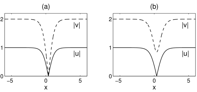
Figure 1: Single dark-dark solitons in Eqs. (1) with $\delta=1,\epsilon=-1$: (a) a degenerate soliton with parameters (57); (b) a non-degenerate soliton with parameters (58).

In the defocusing Manakov equations where $\delta=\epsilon=-1$, their degenerate and non-degenerate single dark solitons qualitatively resemble those shown in Fig. 1, and are thus not shown.

3.2 Collision of two dark solitons

Two-dark-soliton solutions in system (1) correspond to $N=2$ in the general formula (39). In this case, we have

$$u=\mu e^{i[cx-(\delta|\mu|^{2}+\epsilon|\nu|^{2}-c^{2})t]}\frac{G_{2}(x,t)}{F_{2}(x,t)},$$ (59)

$$v=\nu e^{i[dx-(\delta|\mu|^{2}+\epsilon|\nu|^{2}-d^{2})t]}\frac{H_{2}(x,t)}{F_{2}(x,t)},$$ (60)

where

$$F_{2}(x,t) = 1+e^{\theta_{1}+\bar{\theta}_{1}+\rho_{1}}+e^{\theta_{2}+\bar{\theta}_{2}+\rho_{2}}+re^{\theta_{1}+\bar{\theta}_{1}+\theta_{2}+\bar{\theta}_{2}+\rho_{1}+\rho_{2}},$$ (61)

$$G_{2}(x,t) = 1+y_{1}e^{\theta_{1}+\bar{\theta}_{1}+\rho_{1}}+y_{2}e^{\theta_{2}+\bar{\theta}_{2}+\rho_{2}}+ry_{1}y_{2}e^{\theta_{1}+\bar{\theta}_{1}+\theta_{2}+\bar{\theta}_{2}+\rho_{1}+\rho_{2}},$$ (62)

$$H_{2}(x,t) = 1+z_{1}e^{\theta_{1}+\bar{\theta}_{1}+\rho_{1}}+z_{2}e^{\theta_{2}+\bar{\theta}_{2}+\rho_{2}}+rz_{1}z_{2}e^{\theta_{1}+\bar{\theta}_{1}+\theta_{2}+\bar{\theta}_{2}+\rho_{1}+\rho_{2}},$$ (63)

$$\theta_{j}=p_{j}x-ip_{j}^{2}t+\theta_{j0},\quad e^{\rho_{j}}=1/(p_{j}+\bar{p}_{j}),$$ (64)

$$y_{j}=(ic-p_{j})/(ic+\bar{p}_{j}),\quad z_{j}=(id-p_{j})/(id+\bar{p}_{j}),$$ (65)

$$r=1-(p_{1}+\bar{p}_{1})(p_{2}+\bar{p}_{2})/|p_{1}+\bar{p}_{2}|^{2},$$ (66)

and $\mu,\nu,p_{1},p_{2},\theta_{10},\theta_{20}$ are complex constants satisfying the constraint (41) with $j=1,2$, or equivalently, $a_{j}$ is given by the formula (44), where $p_{j}=a_{j}+ib_{j}$.

In generic cases where $\mbox{Im}(p_{1})\neq\mbox{Im}(p_{2})$, these solutions describe the collision of two dark-dark solitons. To demonstrate these collisions, we take parameters

$$\mu=1,\hskip 4.26773pt\nu=2,\hskip 4.26773ptc=0,\hskip 4.26773ptd=0.5,\hskip 4.26773ptp_{1}=0.8426-0.2i,\hskip 4.26773ptp_{2}=1.1801+0.2i,\hskip 4.26773pt\theta_{10}=\theta_{20}=0.$$ (67)

Here the real parts of $p_{1}$ and $p_{2}$ are obtained from the formula (44) with the plus sign. The corresponding two dark-dark soliton solution (59)-(60) is shown in Fig. 2. We can see that after collision, the two dark solitons pass through each other without any change of shape and velocity in either of its two components. Hence the degrees of darkness in each soliton do not change after collision, which means that there is no energy transfer from one component to the other inside each soliton after collision. In addition, there is no energy transfer from one soliton to the other after collision either. This complete transmission of dark solitons’ energy in both its two components after collision occurs not only for $\delta=1$ and $\epsilon=-1$ as in Fig. 2, but also for all other $\delta$ and $\epsilon$ values. Thus it is a common phenomenon of the generally coupled NLS system (1). For instance, it also happens in the defocusing Manakov equations where $\delta=\epsilon=-1$.

This complete transmission of dark-dark solitons’ energy in both its two components is a remarkable phenomenon, because it is in stark contrast with collisions of bright-bright solitons in the same coupled NLS system (1). Indeed, for bright-bright solitons in the focusing Manakov system (with $\delta=\epsilon=1$), polarization rotations take place after collision, hence energy has transferred from one component to the other in each soliton [14]. For bright-bright solitons in the more general coupled NLS system (49) (such as $\delta=1$ and $\epsilon=-1$ above), energy can also transfer from one soliton to another after collision [16]. Thus collisions between bright-bright solitons and between dark-dark solitons in the coupled NLS system (1) are distinctly different.

The reason for this complete energy transmission in all components in dark-soliton collisions is that the intensity profile of each dark-dark soliton is completely characterized by the background parameters $\mu,\nu,c,d$ and the soliton parameter $p_{j}$ [see Eqs. (52)-(53)]. These background parameters are the same for both colliding solitons, and clearly do not change before and after collision. The soliton parameter $p_{j}$ corresponds to the spectral discrete eigenvalue in the inverse scattering transform method, and is a constant of motion throughout collision. Consequently, the intensity profile of each dark-dark soliton (in both $u$ and $v$ components) can not change before and after collision. This property indicates that dark solitons are more robust than bright solitons with regard to collision. The positions of dark solitons do shift after collision though, as can be seen clearly in Fig. 2. This position shift is always toward the soliton’s moving direction, which is the same as collisions of bright solitons in the NLS equation [12].

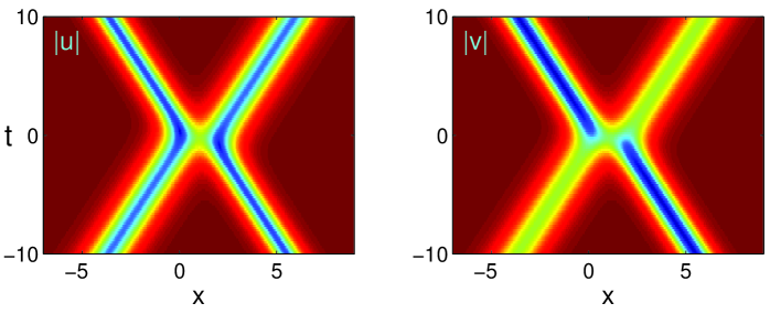
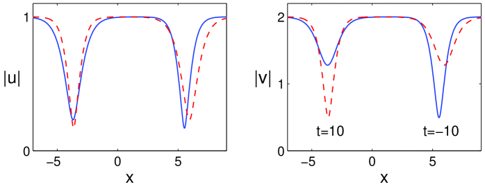
Figure 2: Collision of two dark-dark solitons in Eqs. (1) with $\delta=1,\epsilon=-1$ and parameters (67). The upper row shows the $(x,t)$ evolution, and the lower row shows the intensity profiles before and after collision: $t=-10$ (solid); $t=10$ (dashed).

4 Dark-dark-soliton bound states

In studies of dark solitons, multi-dark-soliton bound states is an interesting subject. In the defocusing NLS equation, two dark solitons repel each other, thus can not form a bound state [40]. In the defocusing Manakov model, multi-bright-dark-soliton bound states were reported in [17]. Some of those bound states are stationary, while the others are not. So far, multi-dark-dark-soliton bound states have never been reported in integrable systems. In a non-integrable system, namely, the second-harmonic-generation (SHG) system, two-dark-dark-soliton bound states do exist, as was reported in [41]. In this system, single dark-dark solitons with non-monotonic tails exist. When two such dark-dark solitons weakly overlap with each other and interact, their non-monotonic tails create local minima in the effective interaction potential, hence the two dark-dark solitons can form stationary bound states. In addition, some of these bound states are stable [41].

In this section, we show that in the generally coupled NLS system (1), when both $\delta$ and $\epsilon$ are negative, i.e., all nonlinearities are defocusing (the defocusing Manakov model), multi-dark-dark-soliton bound states can not exist. But for mixed focusing and defocusing nonlinearities, where $\delta$ and $\epsilon$ have opposite signs, two-dark-dark-soliton bound states do exist and are stationary. To our knowledge, this is the first report of multi-dark-dark-soliton bound states in integrable systems. Properties and physical origins of these stationary bound states in the mixed-nonlinearity model (1) are quite different from the stationary bright-dark-soliton bound states in the defocusing Manakov model [41] and stationary dark-dark-soliton bound states in the non-integrable SHG model [41], as we will explain later in this section.

To obtain dark-dark-soliton bound states, the two dark solitons in the solution (59)-(60) should have the same velocity, i.e., $\mbox{Im}(p_{1})=\mbox{Im}(p_{2})$ (or $b_{1}=b_{2}$), so that the two constituent dark solitons can stay together for all times. In order for this to happen, two different (positive) values $a_{1}$ and $a_{2}$ from Eq. (43) must exist for the same values of $b_{1}=b_{2}$. When $\delta$ and $\epsilon$ are both negative, where the nonlinearities are all defocusing, this is not possible. The reason is that when $\delta<0$ and $\epsilon<0$, the function on the left side of Eq. (43) is an increasing function of $a_{j}^{2}$. Thus for this function to reach the value level of $-2$ on the right side of Eq. (43), there is at most one $a_{j}^{2}$ solution, hence at most one positive $a_{j}$ value. This means that when nonlinearities are all defocusing (i.e., the defocusing Manakov model with $\delta=\epsilon=-1$), there are no multi-dark-dark-soliton bound states. However, when $\delta$ and $\epsilon$ have opposite signs, where focusing and defocusing nonlinearities are mixed, the function on the left side of Eq. (43) may become non-monotone in $a_{j}^{2}$, hence it becomes possible for Eq. (43) to admit two different positive values $a_{1}$ and $a_{2}$ for the same values of $b_{1}=b_{2}$ (see below). In the formula (44), these different $a_{1}$ and $a_{2}$ values correspond to the plus and minus signs respectively. In this case, two-dark-dark-soliton bound states would exist, and this is a new phenomenon in the coupled NLS equations (1) under mixed focusing and defocusing nonlinearities. Physically, these results on bound states in Eqs. (1) can be heuristically understood as follows. We know that in the scalar defocusing NLS equation, two dark solitons repel each other. In the coupled NLS system (1), if $\delta$ and $\epsilon$ are both negative, all nonlinearities are defocusing, hence two dark-dark solitons still repel each other, and no bound states can be formed. However, if $\delta$ and $\epsilon$ have opposite signs, parts of the nonlinear terms are focusing, and the other parts defocusing. While the defocusing terms repel two dark solitons, the focusing terms do just the opposite, which is to attract two dark solitons. Thus, when these repulsive and attractive forces balance each other, two dark-dark solitons then can form a stationary bound state. This physical mechanism for the existence of dark-dark-soliton bound states is quite different from that in the SHG model [41] (see earlier text).

Next we examine these two-dark-dark-soliton bound states in more detail. Through Galilean transformation (i.e., in the moving coordinate system with this common velocity), this common velocity can be reduced to zero. Hence $p_{1}$ and $p_{2}$ become real parameters. In this case, it is easy to see that this bound state becomes

$$\begin{array}[]{ll}u=\mu e^{i[cx-(\delta|\mu|^{2}+\epsilon|\nu|^{2}-c^{2})t]}\frac{G_{2}(x)}{F_{2}(x)},\\ v=\nu e^{i[dx-(\delta|\mu|^{2}+\epsilon|\nu|^{2}-d^{2})t]}\frac{H_{2}(x)}{F_{2}(x)},\end{array}$$ (68)

where

$$F_{2}(x) = 1+e^{2p_{1}x+2\alpha_{1}+\rho_{1}}+e^{2p_{2}x+2\alpha_{2}+\rho_{2}}+re^{2p_{1}x+2p_{2}x+2\alpha_{1}+2\alpha_{2}+\rho_{1}+\rho_{2}},$$ (69)

$$G_{2}(x) = 1+y_{1}e^{2p_{1}x+2\alpha_{1}+\rho_{1}}+y_{2}e^{2p_{2}x+2\alpha_{2}+\rho_{2}}+ry_{1}y_{2}e^{2p_{1}x+2p_{2}x+2\alpha_{1}+2\alpha_{2}+\rho_{1}+\rho_{2}},$$ (70)

$$H_{2}(x) = 1+z_{1}e^{2p_{1}x+2\alpha_{1}+\rho_{1}}+z_{2}e^{2p_{2}x+2\alpha_{2}+\rho_{2}}+rz_{1}z_{2}e^{2p_{1}x+2p_{2}x+2\alpha_{1}+2\alpha_{2}+\rho_{1}+\rho_{2}},$$ (71)

$\alpha_{j}=\mbox{Re}(\theta_{j0})$, and $\rho_{j},y_{j},z_{j},r$ are as given in Eqs. (64)-(66). Notice that functions $F_{2},G_{2}$ and $H_{2}$ are time-independent, thus this bound state is actually stationary. This is analogous to certain bright-dark-soliton bound states in the defocusing Manakov model [17] and dark-dark-soliton bound states in the SHG model [41]. An important feature of these present bound states is that, as $x$ moves from $-\infty$ to $+\infty$, these states acquire non-zero phase shifts. Indeed, it is easy to see from the above solution formula that the phase shifts of the $u$ and $v$ components are

$$u\mbox{-phase shift}=2\phi_{1}+2\phi_{2},\quad v\mbox{-phase shift}=2\chi_{1}+2\chi_{2},$$ (72)

where $2\phi_{j}$ and $2\chi_{j}$ are the phases of $y_{j}$ and $z_{j}$ respectively. In other words, the total phase shifts of the bound state are equal to the sum of the individual phase shifts of the two constituent dark solitons, which are non-zero in general. This contrasts stationary bright-dark-soliton bound states in the defocusing Manakov model [17] and dark-dark-soliton bound states in the SHG model [41], where phase shifts of the dark components across the soliton are all zero.

To demonstrate these stationary two-dark-soliton bound states, we take parameters

$$\mu=1,\hskip 4.26773pt\nu=2,\hskip 4.26773ptc=0,\hskip 4.26773ptd=0.5,\hskip 4.26773ptp_{1}=1.0679,\hskip 4.26773ptp_{2}=0.3311,\hskip 4.26773pt\alpha_{1}=\alpha_{2}=0.$$ (73)

Here $p_{1}$ and $p_{2}$ are obtained from the formula (44) with $b_{1}=b_{2}=0$. The corresponding bound state is displayed in Fig. 3 (upper row). In this bound state, the $u$-component is double-dipped (i.e., has a double hole), signifying this is a two-soliton bound state, while the $v$-component is single-dipped. By adjusting $\alpha_{1}$ and $\alpha_{2}$ values, we can obtain bound states where both $u$ and $v$ components are double-dipped. For instance, when we take $\alpha_{1}=-\alpha_{2}=2$ instead of zero in (73), we get such a bound state which is shown in the lower row of Fig. 3. For both bound states, the total phase shift of the $u$-component is zero, and the total phase shift of the $v$-component is 3.4355, as can be calculated from formula (72).

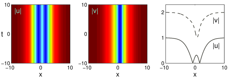
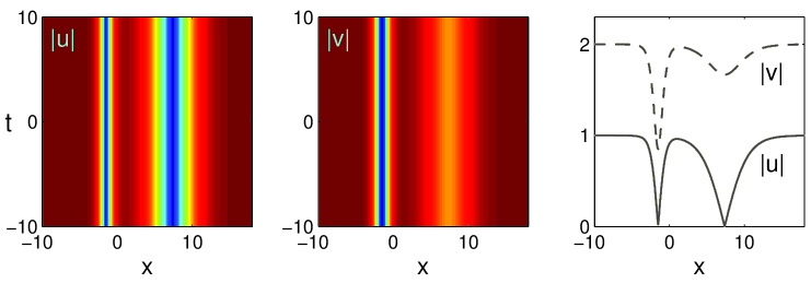
Figure 3: Two examples of two-dark-soliton bound states in Eqs. (1) with $\delta=1,\epsilon=-1$. Upper row: bound state with parameters (73); lower row: bound state with parameters (73) except that $\alpha_{1}=-\alpha_{2}=2$. The left two panels show $(x,t)$ evolution of $|u|$ and $|v|$ components, and the right panel shows the stationary intensity profiles.

From the above analytical formulae and Fig. 3, we can see that these stationary two-dark-soliton bound states have six free parameters, $\mu,\nu,c,d,\alpha_{1}$ and $\alpha_{2}$ [the positive $p_{1}$ and $p_{2}$ values are determined from formula (44) by setting $b_{1}=b_{2}=0$]. The first four parameters characterize the background intensities and phase gradients, while the parameters $\alpha_{1}$ and $\alpha_{2}$ control the positions of the two dark solitons.

The above dark-soliton bound states in the integrable coupled NLS system (1) possess properties which are very different from those in dark-soliton bound states in the non-integrable SHG model [41]. First, the bound states in the SHG model are formed by identical dark solitons (see Fig. 4 in [41]), but the bound states in the coupled NLS system are formed by different dark solitons since $p_{1}\neq p_{2}$ (see lower row of Fig. 3 in this paper). Second, the bound states in the SHG model have zero phase shifts from one end to the other, but the phase shifts of bound states in the coupled NLS system (1) are non-zero in general [see Eqs. (72)]. Thirdly, the bound states in the SHG model have non-zero binding energy, hence can be stable against perturbations [41]. But the bound states in the present coupled NLS system have zero binding energy. Thus under perturbations, the two constituent dark solitons in these bound states generically will split apart, analogously to bright-soliton bound states in the focusing NLS equation.

At this point, one may wonder if three- and higher-dark-dark-soliton bound states exist in the coupled NLS system (1). It turns out that such bound states can not exist. The reason is that, in a bound state, velocities of all constituent solitons must be the same, i.e., all $b_{j}$ [i.e., $\mbox{Im}(p_{j})$] must be the same. In order for three- and higher-dark-soliton bound states to exist, formula (44) must give at least three distinct positive solutions $a_{j}$ for the same $b_{j}$ value. This is clearly impossible, since formula (44) can give at most two distinct positive $a_{j}$ values when the plus and minus signs are taken. Consequently, three- and higher-dark-dark-soliton bound states can not exist in Eqs. (1). Note that in the defocusing Manakov model, non-stationary three and higher bright-dark-soliton bound states exist, but stationary three and higher bright-dark-soliton bound states do not [17]; while in the non-integrable SHG system, stationary three and higher dark-dark-soliton bound states do exist [41].

5 Summary and discussion

In this paper, we have investigated dark-dark solitons in the integrable generally coupled NLS system (1). By reducing the Gram-type solution of the KP hierarchy, we derived the general $N$-dark-dark solitons in this system. We showed that the dark-dark solitons derived previously in the literature are only degenerate cases of these general soliton solutions. We have also shown that when these solitons collide with each other, energies in both components of the solitons completely transmit through. This behavior contrasts bright-bright solitons in this system, where polarization rotation and soliton reflection can occur after collision. In addition, we have shown that when focusing and defocusing nonlinearities are mixed, two dark-dark solitons can form a stationary bound state. These results will be useful for many physical subjects such as nonlinear optics, water waves and Bose-Einstein condensates, where the coupled NLS equations often arise.

The dark-dark solitons obtained in this paper for the generally coupled NLS system (1) are useful for other purposes as well. For instance, it is known that from dark solitons of the defocusing NLS equation, one can obtain homoclinic solutions of the focusing NLS equation through simple variable transformations [42]. Thus, from these dark-dark solitons in this paper, we can obtain homoclinic solutions to these generally coupled NLS equations (1). Since solutions near homoclinic orbits often exhibit chaotic dynamics [42], the homoclinic solutions for the generally coupled NLS equations (1) then can serve as the starting point to understand chaotic behaviors in these systems.

Lastly, we would like to mention that $N$-bright-bright and $N$-bright-dark solitons in the coupled NLS equations (1) can also be obtained by the KP-hierarchy reduction method. But those reductions will be different from the ones in this paper for dark-dark solitons, and will be left for future studies.

Acknowledgments

We thank Dr. Xingbiao Hu for helpful discussions. The work of Y.O. was partly supported by JSPS Grant-in-Aid for Scientific Research (B-19340031, S-19104002). The work of D.S.W. was supported by China Postdoctoral Science Foundation. The work of J.Y. was supported in part by the (U.S.) Air Force Office of Scientific Research under grant USAF 9550-09-1-0228 and the National Science Foundation under grant DMS-0908167.

References

- [1] D.J. Benney and A.C. Newell, Nonlinear wave envelopes, J. Math. Phys. 46, 133 (1967).
- [2] G.P. Agrawal, Nonlinear Fiber Optics, (Academic Press, San Diego, 1989).
- [3] A. Hasegawa and Y. Kodama, Solitons in Optical Communications, (Clarendon, Oxford, 1995).
- [4] M.J. Ablowitz and H. Segur, Solitons and the Inverse Scattering Transform (SIAM, Philadelphia, 1981).
- [5] F. Dalfovo, S. Giorgini, L. P. Pitaevskii, and S. Stringari, Theory of Bose-Einstein condensation in trapped gases, Rev. Mod. Phys. 71, 463 (1999).
- [6] T.-L. Ho and V. B. Shenoy, Hartree-Fock theory for double condensates, Phys. Rev. Lett. 77, 3276 (1996).
- [7] H. Pu and N. P. Bigelow, Properties of two-species Bose condensates, Phys. Rev. Lett. 80, 1130 (1998).
- [8] H. Pu and N. P. Bigelow, Collective excitations, metastability, and nonlinear response of a trapped two-species Bose-Einstein condensate, Phys. Rev. Lett. 80, 1134 (1998).
- [9] I. Goldstein and P. Meystre, A priori definition of maximal CP nonconservation, Phys. Rev. A 55, 2935 (1997).
- [10] G.J. Roskes, Some nonlinear multiphase interactions, Stud. Appl. Math. 55, 231-238 (1976).
- [11] C.R. Menyuk, Nonlinear pulse propagation in birefringent optical fibers, IEEE J. Quantum Electron. 23, 174 (1987).
- [12] V.E. Zakharov and A.B. Shabat, Exact theory of two-dimensional self- focusing and one-dimensional self-modulation of waves in nonlinear media, Zh. E’ksp. Teor. Fiz. 61, 118 (1971) [Sov. Phys. JETP 34, 62 (1972)].
- [13] L.D. Faddeev and L.A. Takhtadjan, Hamiltonian Methods in the Theory of Solitons (Springer Verlag, Berlin, 1987).
- [14] S.V. Manakov, On the theory of two-dimensional stationary self-focusing of electromagnetic waves, Zh. Eksp. Teor. Fiz 65, 1392 (1973) [Sov. Phys. JETP 38, 248-253 (1974)].
- [15] V.E. Zakharov and E.I. Schulman, To the integrability of the system of two coupled nonlinear Schrdinger equations Physica 4D, 270 (1982).
- [16] D.S. Wang, D. Zhang and J. Yang, Integrable properties of the general coupled nonlinear Schrdinger equations, J. Math. Phys. 51, 023510 (2010).
- [17] A.P. Sheppard and Y.S. Kivshar, Polarized dark solitons in isotropic Kerr media, Phys. Rev. E 55, 4773 (1997).
- [18] R. Radhakrishnan and M. Lakshmanan, Bright and dark soliton solutions to coupled nonlinear Schrödinger equations, J. Phys. A: Math. Gen. 28, 2683-2692 (1995).
- [19] B. Prinari, M. J. Ablowitz, and G. Biondini, Inverse scattering transform for the vector nonlinear Schrödinger equation with nonvanishing boundary conditions, J. Math. Phys. 47, 063508 (2006).
- [20] T. Kanna, M. Lakshmanan, P. Tchofo Dinda, and N. Akhmediev, Soliton collisions with shape change by intensity redistribution in mixed coupled nonlinear Schrödinger equations, Phys. Rev. E 73, 026604 (2006).
- [21] M. Vijayajayanthi, T. Kanna, and M. Lakshmanan, Bright-dark solitons and their collisions in mixed N-coupled nonlinear Schrödinger equations, Phys. Rev. A 77, 013820 (2008).
- [22] E. Date, M. Kashiwara, M. Jimbo and T. Miwa, Transformation groups for soliton equations, Nonlinear Integrable Systems—Classical Theory and Quantum Theory, 39-119 (World Scientific, Singapore, 1983).
- [23] K. Takasaki, Geometry of universal Grassmann manifold from algebraic point of view, Rev. Math. Phys. 1, 1-46 (1989).
- [24] E. Date, M. Jimbo, M. Kashiwara and T. Miwa, Operator approach to the Kadomtsev-Petviashvili equation-transformation groups for soliton equations III, J. Phys. Soc. Jpn. 50, 3806 (1981).
- [25] Y. Ohta, Wronskian solutions of soliton equations, RIMS Kokyuroku 684, 1-17 (1989). [In Japanese]
- [26] R. Hirota, The Direct Method in Soliton Theory (Cambridge University Press, Cambridge, 2004).
- [27] S. Miyake, Y. Ohta and J. Satsuma, A representation of solutions for the KP hierarchy and its algebraic structure, J. Phys. Soc. Jpn. 59, 48-55 (1990).
- [28] Y. Ohta, R. Hirota, S. Tsujimoto and T. Imai, Casorati and discrete Gram type determinant representations of solutions to the discrete KP hierarchy, J. Phys. Soc. Jpn. 62, 1872-1886 (1993).
- [29] M. Jimbo and T. Miwa, Solitons and infinite-dimensional Lie algebras, Publ. Res. Inst. Math. Sci. 19, 943-1001 (1983).
- [30] E. Date, M. Jimbo and T. Miwa, Method for generating discrete soliton equations. II, J. Phys. Soc. Jpn. 51, 4125-4131 (1982).
- [31] N.C. Freeman and J.J.C. Nimmo, Soliton solutions of the Korteweg de Vries and the Kadomtsev-Petviashvili equations: the Wronskian technique. Proc. R. Soc. A 389 319 (1983).
- [32] J.J.C. Nimmo, Wronskian determinants, the KP hierarchy and supersymmetric polynomials. J. Phys. A: Math. Gen. 22, pp. 3213-3221 (1989).
- [33] N. C. Freeman, C. R. Gilson, and J. J. Nimmo, Two-component KP hierarchy and the classical Boussinesq equation, J. Phys. A: Math. Gen. 23, 4793–4803 (1990).
- [34] J.J.C. Nimmo, A bilinear Bäcklund transformation for the nonlinear Schrödinger equation. Phys. Lett. A, 99, 279–280 (1983).
- [35] N. C. Freeman, Soliton solutions of nonlinear evolution equations. IMA J. Appl. Math. 32, 125–145 (1984).
- [36] A. Nakamura, A bilinear -soliton formula for the KP equation, J. Phys. Soc. Jpn. 58, 412-422 (1989).
- [37] J.J.C. Nimmo, Darboux transformations for a two-dimensional Zakharov-Shabat/AKNS spectral problem, Inv. Prob. 8, 219-243 (1992).
- [38] V. E. Zakharov, S. V. Manakov, S. P. Novikov, and L. P. Pitaevskii, The Theory of Solitons: The Inverse Scattering Method (Consultants Bureau, New York, 1984).
- [39] V.S. Shchesnovich and J. Yang, General soliton matrices in the Riemann-Hilbert problem for integrable nonlinear equations, J. Math. Phys. 44, 4604 (2003).
- [40] Y.S. Kivshar, Dark solitons in nonlinear optics, IEEE J. Quantum Electron. 29, 250 (1993).
- [41] A.V. Buryak and Y.S. Kivshar, Twin-hole dark solitons, Phys. Rev. A 51, R41 (1995).
- [42] M.J. Ablowitz and B.M. Herbst, On homoclinic structure and numerically induced chaos for the nonlinear Schrödinger equation, SIAM J. Appl. Math. 50, pp. 339-351 (1990).