Dark Energy as Double N-flation—Observational Predictions

Abstract

We propose a simple model for dark energy useful for comparison with observations. It is based on the idea that dark energy and inflation should be caused by the same physical process. As motivation, we note that Linde’s simple chaotic inflation $V=\frac{1}{2}m^{2}\phi^{2}$ produces values of $n_{s}=0.967$ and $r=0.13$, which are consistent with the WMAP 1ς error bars. We therefore propose $V=\frac{1}{2}m_{2}^{2}\phi_{2}^{2}+\frac{1}{2}m_{1}^{2}\phi_{1}^{2}$ with $m_{1}\sim 10^{-5}$ and $m_{2}\leq 10^{-60}$, where $c=1=\hbar$ and the reduced Planck mass is set to unity. The field $\phi_{1}$ drives inflation and has damped by now ($\phi_{1,0}=0$), while $\phi_{2}$ is currently rolling down its potential to produce dark energy. Using this model, we derive the formula $\delta w(z)\equiv w(z)+1=\delta w_{0}(H_{0}/H(z))^{2}$ via the slow-roll approximation. Our numerical results from exact and self-consistent solution of the equations of motion for $\phi_{2}$ and the Friedmann equations support this formula, and it should hold for any slow-roll dark energy.

Our potential can be easily realized in N-flation models with many fields, and is easily falsifiable by upcoming experiments—for example, if Linde’s chaotic inflation is ruled out. But if $r$ values consistent with Linde’s chaotic inflation are detected then one should take this model seriously indeed.

Submitted: 7 December 2011

1 Introduction

Measuring dark energy is one of the most exciting problems in cosmology today. There are a number of expensive programs underway to measure $w,$ the ratio of the pressure to the energy density in dark energy. If dark energy is a pure cosmological constant, then $w=-1$ for all time. Currently, measurements of $w$ are compared to a toy model in which $w$ changes linearly with expansion factor $a$: $w=w_{0}+w_{a}(1-a)$. Observational programs are judged by a figure of merit which includes their ability to measure the quantities $w_{0}$ and $w_{a}$ in this toy model, also known as the Chevallier-Polarski-Linder (CPL) parametrization (Albrecht et al. 2006, Chevallier & Polarski 2001, Linder 2003).

If one parametrizes $w(a)$ in terms of the above toy model, the current $1\sigma$ limits from the 7-year WMAP data combined with BAO+$H_{0}$+SN are $w_{0}=-.93\pm.13,$ and $w_{a}=-.41\pm.72$ (Komatsu et al. 2010). These values are consistent at the $1\sigma$ level with $w_{0}=-1$ and $w_{a}=0,$ which would be a pure cosmological constant.

In the near future, the Sloan III survey should measure the Baryon Acoustic Oscillation (BAO) scale to high accuracy using LRG’s (Luminous Red Galaxies), and should lead to a measurement of $w_{0}$ to an accuracy of $3\%$ (SDSS-III 2008). Using this same dataset, we can use genus topology to measure $w_{0}$ independently to an accuracy of $5\%$ (Zunckel, Gott, & Lunnan 2010, Park & Kim 2009). Supernova studies can achieve similar results (c.f. Riess et al. 1998, Riess et al. 2007, Albrecht et al. 2006).

In the longer term, the $Euclid$ and $WFIRST$ (Wide-Field Infrared Survey Telescope) satellite missions may be able to achieve an accuracy of $1\%$ (Cimatti et al. 2009, Blandford et al 2010). Such observations may continue to point to $w_{0}=-1$ and $w_{a}=0$ with higher and higher accuracy, which would be an important result, but would leave us still in the dark as to the exact nature of dark energy.

More exciting would be if a detectable difference $\delta w_{0}$ between $w_{0}$ and $-1$ is found (i.e. $\delta w_{0}=w_{0}+1$). For this reason, it is desirable to consider simple models, consistent with current data and falsifiable in principle in the near future, in which there is a chance that such a detectable difference may be found. Such models may be used as a guide for interpreting the observations. We therefore propose such a simple model, based on the idea that inflation and dark energy come from the same physical mechanism. This hypothesis is not present in most of the standard theories popular today.

Today, the most popular theory for dark energy is that a string landscape exists with many metastable vacua with different values of $V_{0}$. In this picture, we are currently sitting at the bottom of a potential well whose low point has a vacuum energy density of $V_{0}$. Thus, the accelerated expansion we see in the Universe today is attributed to our current static location at a metastable well in the potential, while in contrast, we have evidence that the accelerated expansion we see in the early Universe is due to slow-roll inflation, where the field is slowly rolling down a potential hill.

Furthermore, for dark energy today, there is supposed to be a complicated potential that is a function of many fields $\phi_{i}$ rather than merely the one field in slow-roll inflation. The kinetic energy in these $\phi_{i}$ fields has damped out and they are no longer changing. A problematic feature of this model is the value of $V_{0}$: $10^{-120}$ (with $c=1=8\pi G=\hbar),$ an extraordinarily small number. The common solution to this problem is to propose that there are of order $10^{500}$ vacuum states with values of $-1<V_{0}<1.$ Then one invokes anthropic effects to argue that it would be difficult for intelligent life to evolve unless $V_{0}\sim 10^{-120}$ (cf. Weinberg 1987, Vilenkin 2003). This is not as satisfying to some physicists as an actual prediction of the amount of dark energy we observe made directly from the physical model.

A final problem with this model is the appearance of Boltzmann brains (see discussion in Gott 2008 and references therein). Briefly, in the far future, the Universe comes to a finite Gibbons and Hawking temperature $T=1/(2\pi r_{0})$, where $r_{0}=(3/V_{0})^{1/2}$, and Boltzmann brains appear. While this problem may be manageable depending on what measure one uses (c.f. deSimone et al. 2010), it is still a problem that must be addressed in the popular $V_{0}$ model.

This paper will be structured as follows. In section 2, we discuss previous models of dark energy and attempts to unify dark energy with inflation, as well as observational evidence for inflation. In section 3, we discuss Linde’s chaotic inflation. In section 4, we propose our double inflation potential based on Linde’s model. In sections 5 and 6, we show how our potential might be realized as an effective N-flationary potential arising from many axion fields, and explain why this may be regarded as preferable. In section 7, we estimate the probability of different deviations from $w=-1$. In section 8, we describe the numerical approach we used to obtain exact values of $\delta w_{0}$ and $w(z)$, and in section 9 we present the results we obtain. In section 10, we conclude.

We use $c=1=\hbar=8\pi G$ throughout, where $G$ is Newton’s constant. In these units, the reduced Planck mass $m_{pl}$ $=(\hbar c/8\pi G)^{1/2}=2.44\times 10^{18}\ GeV$ is equal to unity. These units follow Linde (2002).

2 Previous Dark Energy and Unification Models

2.1 Dark Energy

While a pure cosmological constant $w\equiv-1$ is the simplest model that explains current observations (see Li, Li & Zhang 2010), there are numerous other dark energy models, which we briefly discuss here to place our own approach in context. Broadly, there are scalar-field models such as quintessence, k-essence, a tachyon field, phantom dark energy, dilatonic dark energy, and a Chaplygin gas. Alternatively, there are also proposals that the Universe’s accelerating expansion may stem from modified gravity, effects of physics above the Planck energy, or backreactions of cosmological perturbations. For these models, we direct the reader to the review of Copeland et al. (2006); here we will focus on summarizing the scalar-field models, since our model falls into this category.

Quintessence is characterized by a scalar field that rolls down its potential to produce the accelerated expansion we observe. Slow-roll solutions are possible if certain conditions are satisfied (see Copeland et al. 2006), and both exponential and power-law type potentials are popular. One possible difficulty with quintessence models is that if the field couples to ordinary matter this could lead to time dependence of the constants of nature. In contrast to quintessence, for k-essence, the expansion stems from the kinetic energy in the field (Armendariz-Picon et al. 2001, 2000, 1999). These models have non-canonical kinetic energy terms.

In addition, there are tachyonic fields, which have been a candidate for both inflation and dark energy. For further discussion, we refer the reader to Copeland et al. 2006, Padmanabhan 2002, Bagla et al. 2003, and Abramo & Finelli 2003; the most notable feature of the tachyon models is that the equation of state varies between $0$ and $-1$ regardless of how steep the tachyon potential is; for accelerated expansion, however, one must have a shallow potential compared to $V(\phi)\propto\phi^{-2}$.

The models enumerated above all correspond to $w\geq-1$; however, $w<-1$ has not been observationally disallowed, and this region of parameter-space is generally produced by so-called “phantom” or “ghost” dark energy. These are scalar fields with negative kinetic energy, and suffer from a number of difficulties, most notably quantum instabilities (see Copeland et al. 2006 and references therein). Dilatonic models are attempts to stabilize phantom dark energy (Cline et al. 2004, Gasperini et al. 2002).

Finally, there is the Chaplygin gas, with equation of state $p\propto-\rho^{-1}$, which at early times behaves as a pressureless dust and at late times as a cosmological constant (Copeland et al. 2006). It is thought that the Chaplygin gas would result in a strong Integrated Sachs-Wolfe effect, and hence loss of power in CMB anisotropies; though this can be avoided, the constraints are rather tight (Kamenshchik et al. 2001).

2.2 Inflation

Since our model is based on the idea that inflation and dark energy are the results of the same physical process, we briefly review the evidence for inflation here to contextualize our model. Proposed by Guth in 1981, inflation, the idea that the Universe underwent a period of exponential, super-luminal expansion in the first $10^{-35}$ seconds after the Big Bang, explains many “puzzles.” For instance, the isotropy of the CMB down to one part in $100,000$, even comparing regions that are not causally connected in the standard Big Bang model, is a natural feature of inflation (see Komatsu et al. 2010, Guth 2007).

Further, the Universe is flat down to a few percent (see Tegmark et al. 2004); Dicke and Peebles (1979) point out that to realize this flatness today in the standard Big Bang model, $\Omega_{tot}$ would have had to be unity to 59 decimal places at the Planck time, an extraordinary fine-tuning. But in inflation, the entire observable Universe today came from such a small initial region in comparison to the radius of curvature of the early Universe that flatness arises generically and requires no fine-tuning.

Another piece of evidence for inflation is the absence of magnetic monopoles. All Grand Unified Theories predict them. Indeed, Preskill (1979) estimates they would be dominant in a non-inflationary cosmology. However, none are observed. Inflation provides a natural mechanism to explain why, as the exponential expansion moves the nearest monopoles beyond our observable Universe. Finally, inflation predicts a density spectrum of almost scale-invariant, adiabatic Gaussian fluctuations, a spectrum that fits the observed temperature fluctuations in the CMB as a function of angular scale quite well (Guth & Kaiser 2005, Guth 2007, Komatsu et al. 2010).

Thus it appears we experienced an epoch of accelerated expansion in the early Universe (inflation), and we observe that we are in another epoch of accelerated expansion today due to dark energy. With all of this in mind, it seems the simplest model of dark energy would be one in which it and the inflation we encounter in the early Universe are essentially identical.

2.3 Unification Models

Unification of dark energy and inflation has been proposed before. For instance, Peebles and Vilenkin (1998) used a scalar field potential $V\propto\phi^{4}+m^{4},\ \phi<0,\ V\propto\frac{m^{8}}{\phi^{4}+m^{4}},\ \phi>0,$ which is supposed to produce inflation like a self-interacting field for $\phi<0$ and then dark energy as it slow-rolls for $\phi>0$. Cardenas (2006) proposed a tachyonic field with an exponential potential $V\propto\exp[-\phi/\phi_{0}],$ where there is inflation followed by reheating and finally an epoch of dark energy inflation as $\phi$ continues to roll down the hill of its potential. Finally, Liddle & Urena-Lopez (2006) explore two scenarios: unification of dark matter, dark energy, and inflation into the same scalar field, and unification of dark energy with dark matter in one scalar field while inflation is provided by another.

Double inflation scenarios in which the early Universe undergoes two separate epochs of inflation have also been proposed (these scenarios do not attempt to explain dark energy as coming from an inflaton-like field). For instance, Poletti (1989) considers the quantum cosmology of a mini-superspace model, and focuses on the idea that the Wheeler-DeWitt equation may be invariant under rescalings of the metric. We note this work simply to give credit to Poletti for the idea of a double-inflationary scenario (he also derives the relations showing how the two fields’ evolutions relates to their masses); his focus on the Wheeler-DeWitt equation is very different from our own on dark energy.

Turner et al. (1987) suggest double inflation in the early Universe as an exlanation for a bimodal density fluctuation spectrum (fluctuations on small and large scales) consistent with the observations available in the late 1980’s on galaxy structure. Silk & Turner (1987) make a similar suggestion, arguing that the decoupling of large and small scale structure such a scenario would produce could explain the (circa 1986) excess of observed power on large scales. Muller and Schmidt (1988) propose that double inflation might arise from fourth-order gravity coupled to a scalar field, and suggest that the second epoch of inflation would yield dark matter.

Finally, Polarski & Starobinsky (1992) calculate the spectrum of perturbations produced by double inflation, and are again motivated by the apparent mismatch between theory and observation in prediction of large-scale structure. More recently, Yamaguchi (2001) uses double inflation to explain large-scale structure (first epoch) and small-scale structure (second-epoch), suggesting it might naturally arise from supergravity; Yamaguchi also does not suggest double inflation as an explanation for dark energy.

3 Chaotic Inflation

Let us begin with Linde’s (1983) chaotic inflation, arguably the simplest model of inflation ever proposed. Linde’s potential was of the form

$$V(\phi)=\frac{1}{2}m^{2}\phi^{2}$$ (1)

in Planck units where $c=1=\hbar=8\pi G$, $m_{pl}=(\hbar c/8\pi G)^{1/2}=1$ is the reduced Planck mass, and $G$ is Newton’s constant.

This is a simple massive scalar field. The full equation of motion for the field is

$$\ddot{\phi}+3H\dot{\phi}=-\frac{dV}{d\phi}=-m^{2}\phi,$$ (2)

where $H$ is the Hubble constant and $3H\dot{\phi}$ is a frictional term due to the expansion of the Universe (see Copeland et al. 2006, Linde 2002, Lyth & Liddle 2000). In general, in inflationary models where the Universe is effectively flat,

$$H^{2}=\frac{1}{3}\rho$$ (3)

(with $8\pi G=1$). Taking $\rho$ to be due primarily to the inflationary potential $V(\phi)$, we have

$$H=\sqrt{\frac{1}{3}}\rho^{1/2}\approx\frac{m\phi}{\sqrt{6}},$$ (4)

The approximation follows by noting that in slow-roll inflation, the condition $\dot{\phi}^{2}<<V(\phi)$ is satisfied (see Copeland et al. 2006, Linde 2002). Thus $\rho=\frac{1}{2}\dot{\phi}^{2}+V(\phi)\approx V(\phi)$.

We now make the further approximation that $\ddot{\phi}<<\dot{\phi,}$ which is satisfied because the frictional term $3H\dot{\phi}$ means that the field quickly reaches a nearly constant “terminal” velocity. We thus have from equation (2) that, in the early Universe during the inflationary epoch,

$$\dot{\phi}\approx-\frac{m^{2}\phi}{3H}$$ (5)

Since $H=d\ln{a}/dt$, we have

$$d\ln a=H\frac{dt}{d\phi}d\phi=-\frac{1}{2}\phi d\phi,$$ (6)

where the last equality follows by using equation (4) for $H$ and equation (5) for $dt/d\phi=\dot{\phi}^{-1}.$

If $N$ is the number of e-folds of inflation then

$$N=\ln\frac{a_{final}}{a_{initial}}=-\frac{1}{2}\int\phi d\phi=\frac{1}{4}[\phi_{initial}^{2}-\phi_{final}^{2}].$$ (7)

Inflation continues in slow-roll until $\phi_{final}^{2}=1$, when the kinetic energy $\frac{}{}$$\frac{1}{2}\dot{\phi}^{2}$ becomes comparable with the potential energy $\frac{1}{2}m^{2}\phi^{2}$. At this point, the exponential expansion ends and the kinetic energy in the field is dumped into the thermal energy of particles, ushering in the hot big bang epoch $-$ a radiation dominated, thermal-energy filled Universe. The $\phi$ field is damped and settles at $\phi=0$ during this process, so that $V(\phi)=0$ and the vacuum energy density in the massive scalar field becomes zero. (Or the tiny value of $V_{0}=10^{-120}$ if one adds a tiny constant to the formula such that $V(\phi)=V_{0}+\frac{1}{2}m^{2}\phi^{2}$ to account for dark energy. But we will not be adding this $V_{0}$ term.)

Fluctuations re-entering the causal horizon today left the causal horizon approximately $N=60$ e-folds prior to the end of inflation, when according to equation (7) the value of $\phi^{2}=4N+1=241.$ In this case, the value of the power law primordial tilt evaluated at $k_{0}=.002\,Mpc^{-1}$ should be

$$n_{s}\approx 1+2\left(\frac{V^{\prime\prime}}{V}\right)-3\left(\frac{V^{\prime}}{V}\right)^{2}\approx 1-\frac{8}{\phi^{2}}\approx.967\quad(predicted)$$ (8)

(cf. Easther and McAllister 2006) and the value of $r$, the ratio of tensor to scalar modes, should be

$$r\approx 8\left(\frac{V^{\prime}}{V}\right)^{2}\approx\frac{32}{\phi^{2}}\approx\frac{8}{N}\approx.13\quad(predicted)$$ (9)

(cf. Kim and Liddle 2006). Fitting the amplitude of the observed fluctuations requires

$$m=7.8\times 10^{-6}$$ (10)

(cf. Kim and Liddle 2006). Remarkably, the predicted values of $n_{s}$ and $r$ are consistent with the observed values from WMAP+BAO+$H_{0}$ (Komatsu et al. 2010):

$$n_{s}=.968\pm.012\quad(observed)$$ (11)

and the $95\%$ confidence level constraint

$$r<.24\quad(observed).$$ (12)

The agreement between the predicted and observed values of $n_{s}$ is especially impressive considering that potentials of the form $V(\phi)=(\lambda/4)\phi^{4}$ have been ruled out by predicting unacceptable values of $n_{s}=.95$ and $r=.26$ (cf. Komatsu et al. 2010). Given this, the search for the tensor modes $(r>0)$ is on $-$ for instance, the $Planck$ satellite hopes to improve the measurement of $r$. Polarization studies in the future should if successful offer a smoking-gun proof that the tensor modes are there. Such modes are not predicted by the Ekpyrotic/Cyclic scenario and, if found, they would offer a convincing proof of inflation (cf. Linde 2002).

It is remarkable that a model as simple as Linde’s massive-scalar-field chaotic inflation is currently consistent with the observational data. Linde’s model predicts in particular a value of $n_{s}$ noticeably less than $1$ $-$ a hallmark of slow-roll inflation that is indeed observed.

While more complicated potentials can produce lower values of $r$ (cf. Kallosh and Linde 2010), this comes at the expense of adding more free parameters. The Linde theory, in contrast, is simple enough that it offers the possibility of being confirmed in a dramatic way if the observed value of $r$ is $.13$. If that occurs, we will no doubt conclude that the inflation seen in the early Universe is due to a massive scalar field. In that case, we argue here that we should expect a similar origin for dark energy as well.

4 Double Inflation

4.1 $\delta w_{0}$ in terms of the dark energy scalar field today

We propose the following simple double-inflation potential for inflation and dark energy:

$$V=\frac{1}{2}m_{1}^{2}\phi_{1}^{2}+\frac{1}{2}m_{2}^{2}\phi_{2}^{2}$$ (13)

with $m_{1}\sim 10^{-5}$ and $m_{2}\leq 10^{-60}.$ Double inflation with a potential of this form was introduced (typically with $m_{1}\sim(20\pm 5)m_{2}$) to explain inflation alone (Polarski & Starobinsky 1992, see also Silk & Turner 1987). We will be using it with widely different mass scales to explain inflation and dark energy. The equation of motion for the inflaton field is

$$\ddot{\phi}_{1}+3H\dot{\phi_{1}}+m^{2}\phi_{1}=0,$$ (14)

and for the dark energy field is

$$\ddot{\phi}_{2}+3H\dot{\phi_{2}}+m^{2}\phi_{2}=0.$$ (15)

As noted earlier, we are working in Planck units where $c=1=\hbar=8\pi G$, $m_{pl}=(\hbar c/8\pi G)^{1/2}=1$ is the reduced Planck mass, and $G$ is Newton’s constant.

In the inflationary epoch when the Universe is dominated by the vacuum energy density provided by $V$, we have

$$3H^{2}=V=\frac{1}{2}m_{1}^{2}\phi_{1}^{2}+\frac{1}{2}m_{2}^{2}\phi_{2}^{2}.$$ (16)

The slow-roll approximation is valid for both fields and the evolution of the two fields is given by

$$\ln\frac{\phi_{2}(t)}{\phi_{2,initial}}=\left(\frac{m_{2}^{2}}{m_{1}^{2}}\right)\ln\frac{\phi_{1}(t)}{\phi_{1,initial}}$$ (17)

(cf. Easther & Mcallister 2006). Since $m_{2}<<m_{1,}$ $\phi_{2}(t)\approx constant\approx\phi_{2,initial}$ even though $\phi_{1}(t)/\phi_{1,initial}$ evolves considerably during inflation. There have been $60$ e-folds of inflation since the perturbations now re-entering the horizon left the causal horizon, but there could have been more e-folds of inflation before that, so we expect $N>60$ and thus $\frac{}{}$$\frac{1}{4}[\phi_{1,initial}^{2}-\phi_{1,final}^{2}]=N>60.$ Since $\phi_{1,final}^{2}=1$ marks the end of inflation, $\phi_{1,initial}^{2}>(4\times 60+1)=241.$ As inflation ends, the kinetic energy in the $\phi_{1}$ field is converted into thermal particles, the motion in $\phi_{1}$ damps, and $\phi_{1}$ comes to rest at a value of $\phi_{1}=0.$ The dark energy seen today thus derives from the $\phi_{2}$ field, and $V=\frac{1}{2}m_{2}^{2}\phi_{2}^{2}$ today because $\phi_{1,0}=0$.

Since we observe a dark energy acceleration today consistent with $w\approx-1$ we expect slow-roll inflation to apply $\left[\ddot{|\phi|}<<3H|\dot{\phi|},\ \dot{\phi}^{2}<<V(\phi)\right]$. Since dark energy is dominant today, we use our results from Section 3. Since today $\rho_{DE,0}=\Omega_{DE}\rho_{0}$, $\rho_{0}=(1/\Omega_{DE})\rho_{DE,0}.$ Making these changes to equation (4), we have

$$H_{0}\approx\frac{1}{\sqrt{6\Omega_{DE}}}m_{2}\phi_{2,0},\;\dot{\phi}_{2,0}\approx-\frac{m_{2}^{2}\phi_{2,0}}{3H_{0}}\approx-\sqrt{\frac{2\Omega_{DE}}{3}}m_{2}.$$ (18)

Now, $w$, defined to be the ratio of pressure to energy density in the dark energy, is given by

$$w\equiv\frac{p}{\rho}=\frac{\frac{1}{2}\dot{\phi}_{2}^{2}-V}{\frac{1}{2}\dot{\phi}_{2}^{2}+V},$$ (19)

where the equality is specific to scalar quintessence fields (see Copeland et al. 2006), and we recall that because the inflationary field has damped long ago, $V=\frac{1}{2}m_{2}^{2}\phi_{2}^{2}$ in the present epoch. We therefore have from equations (18) and (19) that

$$w_{0}\approx\frac{\frac{2}{3}\Omega_{DE}-\phi_{2,0}^{2}}{\frac{2}{3}\Omega_{DE}+\phi_{2,0}^{2}}.$$ (20)

The difference between $w_{0}$ and $-1$, which we define to be $\delta w_{0}$, is thus

$$\delta w_{0}\equiv w_{0}+1\approx\frac{4}{(3/\Omega_{DE})\phi_{2,0}^{2}+2}.$$ (21)

Current limits from WMAP suggest $\delta w_{0}=.07\pm.13,$ where $\delta w_{0}$ is simply $\delta w$ today. Importantly, since in the future we expect $\phi_{2}$ to roll down to zero, leaving a vacuum energy density of zero (with no $V_{0}$ term), the Boltzmann brain problem disappears. See Figure 2 for a comparison of this formula to our numerical results from a full and self-consistent solution of the equation of motion for $\phi_{2}$ and the Friedmann equation as described in Section 8. Equation (21) is only valid evaluated today, because today we are dark-energy dominated, which is the assumption under which this formula was derived. This formula will not be valid as a function of time in the past, because dark energy has only recently become dominant.

4.2 $\delta$w as a function of redshift

In what follows, we will derive a formula that gives $\delta w$ as a function of time. Let us be very clear here that we are no longer assuming dark-energy domination as we did in 4.1.

The formula we present below will give $\delta w(z)$ as a function of $H(z)$ and so is a simple template observational programs can use to look for slow-roll dark energy.

We have from equation (19) and the definition $\delta w=w+1$ that

$$\delta w=\frac{\dot{\phi}_{2}^{2}}{(1/2)\dot{\phi}_{2}^{2}+V}.$$ (22)

From this, we can see that small $\delta w$ implies that $\dot{\phi}^{2}<<V$, and so we approximate that

$$\delta w\approx\frac{\dot{\phi}_{2}^{2}}{V}.$$ (23)

Since $\dot{\phi}_{2}$ is small, $\phi_{2}$ does not vary much with time and so $V$ is approximately constant in time. Thus $\delta w\propto\dot{\phi}_{2}^{2}.$ Since in slow-roll $\ddot{\phi}_{2}$ is also small, we have from equation (15) that

$$3H\dot{\phi}_{2}\approx-\frac{\partial V}{\partial\phi_{2}}=-m_{2}^{2}\phi_{2}.$$ (24)

As we have already noted, $\phi_{2}$ is approximately constant. Hence $3H\dot{\phi}_{2}\approx constant$, so

$$\dot{\phi}_{2}\propto\frac{1}{H}.$$ (25)

Since $\delta w\propto\dot{\phi}_{2}^{2}$, equation (25) implies that

$$\delta w\propto\frac{1}{H^{2}}.$$ (26)

Normalizing appropriately, we obtain

$$\delta w(z)\approx\delta w_{0}\left(\frac{H_{0}}{H(z)}\right)^{2}.$$ (27)

In summary, then, for small $\delta w$, slow-roll applies, $\dot{\phi}_{2}$ is small, and $\delta w\propto\dot{\phi}_{2}^{2}.$ When the field reaches terminal velocity, the acceleration $\ddot{\phi}_{2}$ is nearly zero, so the Hubble friction term $3H\dot{\phi}_{2}$ is balanced by the slope of the potential the field is rolling down, $-\partial V/\partial\phi_{2}$. This is analogous to a ball rolling down a hill: it will reach terminal velocity when energy dissipation from friction cancels out the energy it gains by moving to lower values of its potential. Finally, if $\phi_{2}$ is roughly constant in time, $\partial V/\partial\phi_{2}$ will be as well, meaning $\dot{\phi}_{2}\propto H^{-1}$, which leads to equation (26). This derivation could easily be duplicated for other dark energy potentials as long as $\delta w$ is small.

We term this formula (equation (27)) our "slow-roll formula” in subsequent discussion. See Figure 3 for a comparison of this formula to our numerical results from a full and self-consistent solution of the equation of motion for $\phi_{2}$ and the Friedmann equation as described in Section 8.

5 N-flation

A potential of the form in equation (13) governed by equations of motion (14) and (15) can be produced easily by models of N-flation. A possible criticism of the original Linde chaotic inflation is that it requires $\phi>1$ in Planck units. Linde argued that this was acceptable as long as $V<1.$ But it was felt that it would be difficult to produce values of $\phi>1$ in string theory models. Thus, N-flation (Dimopoulos et al. 2008) has been proposed (cf. also Easther and McAllister 2006), motivated by the fact that supersymmetric string theories allow of order $10^{5}$ axion fields.

For such axion fields $V(\psi_{i})=\mu^{4}[1-\cos(\psi_{i}/f_{i})]$, and for $\psi_{i}<<1$ (i.e. $\psi_{i}$ significantly below the Planck mass $-$ which we would like) we note that the potential is of the Linde quadratic form with effective mass $m=\mu^{2}/f_{i}$. As we have already pointed out, string theory allows the number of such fields to be large (Dimopoulos et al. 2005). Hence in this work we will adopt $N=10^{4}$.

In this model there are $N$ fields $\psi_{i}$ (where $i=1,\,.\,.\,.\,,\,N$) with approximately equal masses $m_{i}\approx m$. Then the potential is $V=\sum\frac{1}{2}m_{i}^{2}\psi_{i}^{2}\approx V(\phi)=\frac{1}{2}m^{2}\phi^{2}$ where $\phi^{2}\equiv\sum\psi_{i}^{2}$. This is so-called "assisted inflation."

Since each $m_{i}\approx m$, all the $\psi_{i}$’s evolve together via

$$\ln\left[\frac{\psi_{i}(t)}{\psi_{i,initial}}\right]=\left(\frac{m_{i}^{2}}{m_{j}^{2}}\right)\ln\left[\frac{\psi_{j}(t)}{\psi_{j,initial}}\right]\approx\ln\left[\frac{\psi_{j}(t)}{\psi_{j,initial}}\right]$$ (28)

if $m_{i}\approx m_{j}$ for all $i$ and $j.$ This will be true if the mass spectrum of the fields is strongly peaked and densely packed:

$$m_{i}^{2}=m^{2}\exp\left[(i-1)/\sigma\right],$$ (29)

where $\sigma>280$ for $N>600$ (Kim and Liddle 2006). If the fields are strictly non-interacting the masses could in fact be exactly equal.

We want double N-flation with a potential

$$V=\sum\frac{1}{2}m_{1}^{2}\psi_{1,i}^{2}+\sum\frac{1}{2}m_{2}^{2}\psi_{2,i}^{2}=\frac{1}{2}m_{1}^{2}\phi_{1}^{2}+\frac{1}{2}m_{2}^{2}\phi_{2}^{2}$$ (30)

where there are $N=10^{4}$ $\psi_{2}$ fields each of mass $m_{2}\approx 10^{-60}$ and $N=10^{4}$ $\psi_{1}$ fields each of mass $m_{1}\approx 10^{-5}$ (in keeping with our hypothesis that inflation and dark energy should arise from the same process) and by definition $\phi_{2}^{2}=\sum\psi_{2,i}^{2}$ and analogously for $\phi_{1}^{2}.$ Initially we need $\phi_{1,initial}^{2}>241$ to produce enough inflation ($>60$ e-folds) to explain our Universe. With $10^{4}$ fields, that just means that each $\psi_{1,i}^{2}>.0241$ and so all the $\psi_{1,i}$’s can be sub-Planckian ($<1$). This is good.

Are such low values of $m_{2}\approx 10^{-60}$ plausible from the point of view of string theory? Interestingly, Kaloper and Sorbo (2006) have independently proposed just such an N field quiNtessence model for dark energy using ultralight pNGB [pseudo-Nambu Goldstone bosons] (axions) from string theory. They argue for potentials of the form $V(\psi_{i})=\mu^{4}[1-\cos(\psi_{i}/f_{i})]$. Svrcek (2006) has also argued for multiple ultra-light axion fields with potentials of this form to explain dark energy.

We note in each case that for sub-Planckian $\psi_{i,initial}$’s, the potential is of the desired Linde quadratic form with effective mass $m=\mu^{2}/f_{i}$. Svrcek notes that pseudoscalar axion fields have a shift symmetry and if this symmetry were exact it would set the potential to zero and the axions would be massless. In string theory the shift symmetry is broken only by nonperturbative effects. In string theory axions thus receive potential only from nonperturbative instanton effects which are exponentially suppressed by the instanton action. Hence, if the instantons have large actions they can give rise to a potential many orders of magnitude below the Planck scale.

Svrcek argues that $\mu^{4}=M^{4}\exp[-S_{inst}],$ where $M\sim 1$ and $S_{inst}\sim 280,$ can create a vacuum energy density today comparable with what we observe for dark energy. Svrcek adds a $V_{0}$ term as well, which we eliminate as unnecessary. We argue that if the axion fields are able to explain the amount of dark energy we observe today the $V_{0}$ term can be eliminated. Both Kaloper and Sorbo (2006) and Svrcek (2006) are explicitly creating quintessence models for dark energy. Both also note that single field models with sub-Planckian field values are unacceptable for quintessence and favor models with $N=10^{4-5}$ fields.

We are proposing to combine these quintessence models that use $N$ fields with the N-flation models to explain dark energy $and$ inflation. Independently Svrcek (2006) also speculates “Hence, it could be that some of the string theory axions have driven inflation while others are currently responsible for [a] cosmological constant.” We take the point of view here that there are $N=10^{4}$ equal-mass ultra-light fields $\psi_{2,i}$ that create a slow-roll dark energy and $N=10^{4}$ equal-mass heavy fields $\psi_{1,i}$ that create slow-roll inflation in the early Universe.

If there are in addition singleton fields with intermediate masses, with sub-Planckian $\psi_{i}$’s also, these would not have inflated but rather would have rolled down, as Svrcek notes. Some of these axion fields could have rolled down and created dark matter. They do not cause inflation because $\psi_{i}<1$, so when the other thermal particles redshift so that the $\psi_{i}$ vacuum field energy becomes dominant, $3H^{2}=\frac{1}{2}m_{i}^{2}\psi_{i}^{2}$. Thus $H$ is not large enough to cause the low velocity ($\dot{\psi_{i})}$ required for slow-roll inflation.

However, if there are many fields of essentially the same mass, $3H^{2}=\sum\frac{1}{2}m_{i}^{2}\psi_{i}^{2}\approx\frac{1}{2}m^{2}\phi^{2},$ where $\phi^{2}>1$. In this case, $H$ is much higher (by a factor of $\sqrt{N}$) causing each $\dot{\psi}_{i}$ to be lower and slow-roll inflation to occur. Thus, inflation only occurs when many fields congregate at the same mass scale.

6 Why N-flation is superior

We expect all of the $\psi_{2,i}$’s and $\psi_{1,i}$’s to be sub-Planckian. If $N=10^{4}$, this means that $\phi_{i,initial}^{2}<10^{4}$, which means (using equation 7) that there can be at most 2500 e-folds of inflation in our Universe. Hence our Universe today is less than $\exp[2440]$ times larger than the visible horizon. In Linde’s original formulation of chaotic inflation, random quantum fluctuations allowed Universes to give birth to Universes with various values of $\phi_{1,initial}$. The ones with larger values of $\phi_{1,initial}$ grew faster until most of the volume of the multiverse was in the fastest expanding states, with $V=1=\frac{1}{2}m_{1}^{2}\phi_{1}^{2}.$ That would mean $\phi_{1,initial}^{2}\approx 10^{10}$ and the Universe today would be $\exp[10^{10}]$ times larger than the part we can see.

For our model of dark energy, a simple Linde-type chaotic double-inflation picture would eventually lead to most of the volume of the multiverse being in the fastest expanding states, given by the ellipse

$$V=1=\frac{1}{2}m_{1}^{2}\phi_{1}^{2}+\frac{1}{2}m_{2}^{2}\phi_{2}^{2}$$

$$=\frac{\phi_{1}^{2}}{2\times\left(10^{5}\right)^{2}}+\frac{\phi_{2}^{2}}{2\times\left(10^{60}\right)^{2}}.$$ (31)

This ellipse is very elongated in the $\phi_{2}$ direction, and at random points on it the $\phi_{2}$ field contributes just as much to the potential and to the inflation as the $\phi_{1}$ field. Thus starting values $\phi_{2,initial}\approx(m_{1}/m_{2})\phi_{1,initial}$ would be expected, and since $\phi_{2}$ is slower to roll down than $\phi_{1},$ we would not get the sub-dominant dark energy we require.

If we use N-flation to realize the potential in equation (13) via equation (30) this problem does not occur. Since all of the fields are sub-Planckian, the fastest inflating regions are characterized by starting values of $\phi_{2}^{2}\approx\phi_{1}^{2}$ that are bounded above by $N$, and since $m_{2}<<m_{1}$, the contribution of the $\phi_{2}$ field to the potential is sub-dominant ($<\frac{1}{2}m_{2}^{2}N$ for the $\phi_{2}$ field versus $<\frac{1}{2}m_{1}^{2}N$ for the $\phi_{1}$ field).

7 Bound on probabilities for deviation of w from $-1$

In this picture we might expect the initial values for $\phi_{2}^{2}$ and $\phi_{1}^{2}$ to be comparable. What is the smallest $\phi_{1,initial}^{2}$ could be? It must be at least 241 to explain the at least 60 e-folds of inflation we see within the visible Universe. By the above argument, we might expect $\phi_{2,initial}^{2}$ to be similar. Because of equation (17), $\phi_{2}$ does not evolve much during the period of inflation. Its main chance to roll down is in the current epoch when $H$ is low. But there have not been many e-folds of inflation during the current epoch, so we might expect $\phi_{2,0}^{2}$ to be only a little less than its minimal initial value of about $241$. That would give a value today of $\delta w_{0}\approx 4/\left(\left(3\phi_{2,0}^{2}/\Omega_{DE}\right)+2\right)=.4\%$ via equation (21).

Since we expect the $\psi_{2,i}$’s and the $\psi_{1,i}$’s of equation (30) to be uncorrelated in our n-flationary picture, we expect by the central limit theorem that $\phi_{2,initial}$ and $\phi_{1,initial}$ are Gaussian. If their magnitudes are comparable, in keeping with our hypothesis that the physical processes for inflation and dark energy are identical, we might a priori expect on average to find $<\phi_{2,initial}^{2}>\>=\><\phi_{1,initial}^{2}>.$

Consider the probability function $P(\phi_{2,initial},\phi_{1,initial})d\phi_{2,initial}d\phi_{1,initial}.$ If both variables follow a Gaussian distribution, $P$ has circular probability contours in the $(\phi_{2,initial},\,\phi_{1,initial})$ plane, and the probability of finding $|\phi_{2,initial}|<X|\phi_{1,initial}|$ for $X<1$ is simply $P=(2/\pi)\arctan X$. If $\phi_{1,initial}^{2}>241,$ the probability of observing a value of $\delta w_{0}>\delta w_{0}^{\prime}$ is

$$P(\delta w_{0}>\delta w_{0}^{\prime})<\frac{2}{\pi}\arctan\left[\frac{1}{\sqrt{241}}\sqrt{\frac{\Omega_{DE}}{3}\left[\frac{4}{\delta w_{0}^{\prime}}-2\right]}\right]$$ (32)

using equation (21) to relate $\phi_{2,0}\simeq\phi_{2,initial}$ to $\delta w_{0}$. See Fig. 1. The probability of observing $\delta w_{0}>3\%$ is $P<20\%.$ It could be considerably smaller if there are significantly more than the minimum 60 e-folds of inflation in the early Universe.

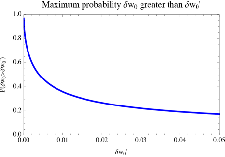
Figure 1: Plot of our upper bound on the probability that $\delta w_{0}$ is greater than a given value (equation (32)). This is an upper bound because in fact $\phi_{1,initial}$ could be much greater than $16$ (chosen to provide approximately the minimal 60 e-folds of inflation), leading to larger values of $\phi_{2}$ and lower values of $\delta w_{0}$. However, the plot is moderately encouraging: there still could in principle be a nearly $20\%$ chance that $\delta w_{0}$ could be as large as $3\%$, which would likely be detectable.

With this in mind, it may be reasonable to expect a small value of $\delta w_{0}$. On the assumption that the same physical processes led to both inflation and dark energy, if there were at least $60$ e-folds of inflation in the early Universe, there should be at least $60$ e-folds of inflation due to dark energy ahead in the future, as indicated in the calculation above. However, the number of galaxies (and observers like ourselves) produced in our Universe is proportional to

$$\exp[3N]=\exp\left[\frac{3}{4}\left(\phi_{1,initial}^{2}-1\right)\right].$$ (33)

So it might not be surprising for us to observe
$<\phi_{2,initial}^{2}>$ less than $<\phi_{1,initial}^{2}>$, but the details depend on questions of measure which are unsettled.

Suffice it to say, one must find a measure that makes what we observe, namely $\phi_{2,initial}^{2}\gtrsim 12$ (since $\delta w_{0}=7\%\pm 13\%$ from WMAP) and $\phi_{1,initial}^{2}>241$ (to produce at least $60$ e-folds of inflation), not particularly unlikely. For the time being, we suggest taking an empirical approach and asking what future observations can tell us about $\phi_{2,initial.}$

8 Numerical Method

To integrate the equation of motion for $\phi_{2}$ (15) numerically, we must also solve the Friedmann equation for $H$ as a function of time. Since we know from observational constraints that $\delta w$ is small, we start by assuming that $w=-1$ and solve the Friedmann equation to determine $H$ as a function of time. Then using this $H$ we can solve the full equation of motion for $\phi_{2}$ as a function of time (though we will instead solve the re-scaled equation (43) as described later in this section). Knowing $\dot{\phi}_{2}$ gives us $w$ as a function of time, and we can insert this back into the Friedmann equation to give us an improved $H$ as a function of time.

We then iterate. This approach converges rapidly on a self-consistent solution where we have $w,\ H,$ and $\phi_{2}$ as functions of time and both the Friedmann equations and the equation of motion for the field $\phi_{2}$ have been solved self-consistently and exactly.

For starting conditions at $t=0$ we assume $d\phi_{2}/dt$=0 since $H(t)$ tends to infinity as $t$ tends to zero. We discuss the starting condition on $\phi_{2}$ itself later. Since in this section we will consider only the $\phi_{2}$ field with mass $m_{2},$ for greater legibility we suppress the subscripts on $\phi_{2}$ and $m_{2}$ in what follows. We recall equation (15) (with subscripts suppressed):

$$\ddot{\phi}+3H\dot{\phi}+m^{2}\phi=0,$$ (34)

where $H=(1/a)(da/dt)$ is the Hubble constant. Defining a new variable for time $\tau=t/t_{H0}=tH_{0}$ and transforming $\ddot{\phi}$ and $\dot{\phi}$, we have $\ddot{\phi}=\phi^{\prime\prime}H_{0}^{2}$ and $\dot{\phi}=\phi^{\prime}H_{0}$, where prime denotes a derivative with respect to the new time variable $\tau$. We thus have from equation (34) that

$$\phi^{\prime\prime}+3\frac{H(t)}{H_{0}}\phi^{\prime}+\frac{m^{2}}{H_{0}^{2}}\phi=0.$$ (35)

$\phi$ and its derivatives are functions of $\tau$, so we desire that $H$ should be as well. We convert the Friedmann equation from time variable $t$ to time variable $\tau$; so doing will yield the Friedmann equation governing $H(\tau)\equiv H(t)/H_{0}$.

It is

$$H^{2}(\tau)\equiv\big{(}\frac{1}{a}\frac{da}{d\tau}\big{)}^{2}=\big{(}\Omega_{r}a^{-4}+\Omega_{m}a^{-3}$$ (36)

$$+\;\Omega_{DE}\exp\left[3\int_{\tau}^{\tau_{0}}H(\tau^{\prime})\left[(1+w(\tau^{\prime})\right]d\tau^{\prime}\right]\big{)},$$

where $\Omega_{r}\equiv\rho_{r}/\rho_{c}$, and analogously for $\Omega_{m}$ and $\Omega_{DE}$. $\rho_{c}\equiv 3H_{0}^{2}/(8\pi G)$ is the critical density; subscript $r$ denotes radiation, $m$ matter, and $DE$ dark energy. $\tau_{0}$ is the value of $\tau$ today (when $a=1$). Note that for $w\equiv-1,$ this reduces to the usual Friedmann equation used in $\Lambda CDM$ models. We thus find the equation for $\phi$

$$\phi^{\prime\prime}+3H(\tau)\phi^{\prime}+m_{*}^{2}\phi=0,$$ (37)

where we have defined $m_{*}^{2}=m^{2}/H_{0}^{2}$.

In principle, we can now solve the Friedmann equation numerically for $H(\tau)$ and using it obtain $\phi$ numerically. However, there is a constraint on $\phi_{2,0}$ that we must satisfy as we solve numerically. The Universe is flat with $\Omega_{DE}+\Omega_{M}\approx 1$. Since dark matter is present, the value of $H_{0}^{2}$ is larger than it would be if only dark energy were present by a factor of $\Omega_{DE}^{-1}$; WMAP-7 gives $\Omega_{DE}=.73$ (Komatsu et al. 2010). Thus at present

$$3H_{0}^{2}=\frac{1}{2\Omega_{DE}}m^{2}\phi_{0}^{2}X,$$ (38)

where $X\equiv(\dot{\phi_{0}}^{2}+m^{2}\phi_{0}^{2})/m^{2}\phi_{0}^{2}.$

Using the definitions of $w$ and $\delta w$, we find that

$$m_{*}^{2}=\frac{3\Omega_{DE}(2-\delta w_{0})}{\phi_{2,0}^{2}}.$$ (39)

Hence we are not free to choose both $m_{*}$ and $\phi_{2,initial}$ independently because $\phi_{2,initial}$ will determine $\phi_{2,0}$, which must be consistent with $m_{*}$ such that equation (39) is satisfied. We therefore require a method of solving the equation of motion where we can set $\phi_{2,initial}$ (and hence $\phi_{2,0}$) after we already have a solution. This motivates us to observe that the equation can be dynamically rescaled by writing $\phi^{\prime}/\phi=\zeta(\tau)$. It is evident that $\phi$ is always non-zero. Writing $\phi^{\prime}=\zeta\phi$, we find that $\phi^{\prime\prime}=\left(\zeta^{2}+\zeta^{\prime}\right)\phi$. Substituting these relations into equation (37), we obtain

$$\zeta^{2}+\zeta^{\prime}+3H(\tau)\zeta+m_{*}^{2}=0.$$ (40)

We choose $m_{*}$ and numerically solve this equation beginning at $\tau=0$, where we have $\zeta=0$ because of our earlier comment on $\dot{\phi}_{2,initial}.$ This is done iteratively in conjunction with the solution of equation (36) as in the overview at the beginning of this section, and in greater detail below; the final iteration gives us $\delta w_{0}.$ We can then determine $\phi_{2,0}$ by inverting equation (39).

We have already given an overview of our iterative procedure; here we give details. As noted before, we begin by finding $H$ as a function of $\tau$ for $w=-1$, which we do using the Friedmann equation (36). For $w=-1$, this does not require knowing $\tau_{0}$. However, solving for $\tau_{0}$ $(\equiv\tau$ such that $a=1$) in this first iteration does provide $\tau_{0}$ for the next round of iteration, where we will use $w=w(\tau)$ in equation (36). We use $H$ as provided by (36) in the dynamically rescaled equation (40) for $\zeta\equiv\phi^{\prime}/\phi$, which yields $w=(\zeta^{2}-m_{*}^{2})/(\zeta^{2}+m_{*}^{2})$ via equation (19). We insert this $w(\tau)$ back into (36) and find a new $H$, which goes back into (40), again yielding $w$. We continue this process until the difference between the $n^{th}$ and $n+1^{th}$ step integrated over all time is negligible compared to $\delta w_{0}$. Then we have an exact and self-consistent solution to the equation of motion for the $\phi_{2}$ field and the Friedmann equation.

9 Numerical Results

In this section, we discuss our numerical results. Figure 2 compares our approximate formula for $\delta w_{0}$ as a function of the value of the dark energy scalar field today, (equation (21)), to our numerical results from exact and self-consistent solution of the Friedmann and scalar field equations, described in Section 8. The curves have similar shapes. However, the approximate formula is not a good substitute for the full numerical results in the range $4<\phi_{2,0}<12$. For $\phi_{2,0}>12$, the match between analytical and numerical is somewhat better. Since our approximate formula was derived in the limit that $\delta w_{0}<<1$, it is not surprising that it agrees better with the full numerical results the smaller $\delta_{w,0}$ becomes.

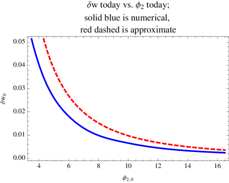
Figure 2: Plot comparing the “back-of-the-envelope” approximate formula $\delta w_{0}=4/(\frac{3}{\Omega_{DE}}\phi_{2,0}^{2}+2)$ with the numerical results obtained as outlined in Section 8. The plot shows that, while the back-of-the-envelope calculation captures the order-of-magnitude of $\delta w_{0}$ and the rough shape of the curve, it should not be trusted in lieu of the numerical results. Since it was derived on the assumption that $\delta w_{0}<<1$, it makes sense that the approximate and numerical results are closer in this region of the plot (i.e. for larger $\phi_{2,0}$).

Figure 3 compares our "slow-roll formula" (equation (27)) with our full numerical results from exact and self-consistent solution of the Friedmann and scalar field equations. Note that the function $H$ used in these plots comes in each case from the self-consistent solution of the Friedmann equation as described in section 8. The "slow-roll" formula agrees well with our numerical results and best for $\delta w_{0}\lesssim 1\%$. Analogously to our discussion of Figure 2, this is not surprising because the "slow roll formula" was derived in the same limit that $\delta w_{0}<<1$. Hence the smaller $\delta w_{0}$ is, the better we would expect the agreement to be.

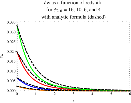
Figure 3: Here, we show our numerical results for $\delta w$ as a function of redshift and also the "slow-roll formula" (dashed) $\delta w=\delta w_{0}\left(\frac{H_{0}}{H(z)}\right)^{2}$ (see Section 4 for derivation). The values of $\phi_{2,0}$ listed on the plot go 16, 10, 6, and 4 from bottom to top for the solid curve/dashed curve pairs. For smaller $\delta w_{0}$ the assumptions underlying our "slow-roll formula" are better satisfied, and one can see it agrees more closely with the numerical results in this regime.

Figure 4 compares a representative result from our model (with $\delta w_{0}=2\%$) to the Chevallier-Polarski-Linder parametrization, $w=w_{0}+w_{a}(1-a)$. We chose the parameters $w_{0}$ and $w_{a}$ so that the toy model agrees with ours at $a=1$ and at $a=0$ (today and at the Big Bang). This leads to $w_{0}=-1+\delta w_{0}$ and $w_{a}=-\delta w_{0}.$ Since the CPL parametrization is the shallower curve in the plot, it is clear that if our model is correct, it will be harder to observe $w$ different from $-1$ in the past than if the CPL parametrization is right. A comparison of Figures 3 and 4 shows that our slow-roll formula provides a much better fit for our numerical results than the CPL parametrization, as it has a physical motivation from the slow-roll approximation.

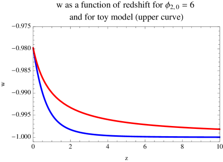
Figure 4: Here, we compare our model’s predictions for $w$ as a function of redshift to those of the popular toy model $w=w_{0}+w_{a}(1-a),$ where $w_{0}$ and $w_{a}$ are constants and $a$ is the scale factor appearing in the Friedmann equation. The toy model, fit at both ends, is the shallower, upper curve. The comparison shows that it will be harder to observe deviations from $w=-1$ in the past if our model is correct than if the toy model is correct.

Figure 3 tells a story consistent with Figure 2: the larger $\phi_{2,0}$ is, the smaller is $\delta w_{0}$. The main take-away is that $\delta w$ is a quite steep function of redshift; as the figure shows, $\delta w$ is nearly indistinguishable from $-1$ for $z\gtrsim 3$ for all of the curves (different curves correspond to different values of $\phi_{2,0}$.) This means that if our model is correct, it will be very challenging to observe deviations of $w$ from $-1$ except in the recent past. If our model is correct, it will also be more challenging to observe deviations from $w=-1$ than if we assumed that $\delta w$ was constant and non-zero.

Note that the initial values of $\phi_{2}$ to which the curves in Figure 3 correspond are roughly the same as the final values we have quoted in the Figure: ($\phi_{2,initial}\simeq\phi_{2,0})$. This is because the Hubble friction ensures that $\phi_{2}$ does not roll down much (see equation (15)). We chose $\phi_{2,0}=16$ on the assumption that $\phi_{2,0}\simeq\phi_{2,initial}\simeq\phi_{1,initial}$ and $\phi_{1,initial}\simeq$16 because that is the minimum value that can provide approximately $60$ e-folds of inflation. The other values of $\phi_{2,0}$ were chosen to illustrate larger values of $\delta w_{0}$.

Figure 5 shows $dw/dz$, which, since $w=\delta w-1$, is the same as $d\delta w/dz$. This plot is consistent with what we might expect from Figure 3: it is only for $z\lesssim 3$ that $dw/dz$ is significantly non-zero.

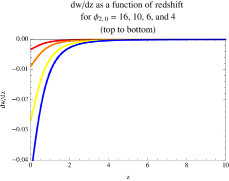
Figure 5: Plot of $dw/dz$ as a function of redshift. The values of $\phi_{2,0}$ are listed in the order that the curves go top to bottom ($\phi_{2,0}=16$ is the red curve, $\phi_{2,0}=10$ is the orange curve, etc.), and chosen to be the same as those in Figure 3.

We note here that others who have studied a variety of quintessence models near either maxima or minima in the potential have obtained approximate analytical solutions for the evolution of $w(a)$ (Dutta & Scherrer 2008, Dutta et al. 2009, Chiba et al. 2009, Huang, Bond, & Kofman 2011). They have also concluded, as we will, that in these models $w(a)$ is not well-fit by any linear function, including the popular toy model $w(a)=w_{0}+w_{a}(1-a)$. Chiba in particular shows that the results of Dutta and Scherrer should apply to a quadratic potential such as the one we use.

10 Conclusion

In this paper, we have argued that the accelerated expansion in the early Universe (inflation) and the accelerated expansion today (dark energy) are caused by the same physical mechanism. If inflation is slow-roll, then dark energy should also be slow-roll, and this allows us a chance to observe a detectable difference $\delta w$ between $w$ and $-1$. We have suggested that the simplest model of inflation, Linde’s chaotic inflation, where the potential is quadratic, could also effectively model dark energy. For those who consider the super-Planckian values of the scalar field in this model problematic, we have suggested that the quadratic potential for inflation and the second quadratic potential we use for dark energy could both be realized as N-flation describing many sub-Planckian fields that are closely clustered in mass.

The idea that dark energy and inflation are caused by the same mechanism produces a real gain in predictive power. Since we know the minimum value of the scalar field for inflation to give the 60 e-folds of inflation we see in the observable Universe, we can, on the reasonable assumption that the two scalar fields would have similar initial values following a Gaussian distribution, estimate upper limit probabilities for observing different values of $\delta w_{0}\equiv w_{0}+1$ today.

We also are able to use this slow-roll dark energy idea to make another prediction: that $\delta w\propto 1/H^{2}$. Figure 3 shows, our numerical results seem to follow this formula. Our analytical work shows that this is generically true in any slow-roll model of dark energy. This relationship can, we hope, provide a valuable template to observers seeking to look for a signal in noisy data. Indeed, if observers find this shape for $w(z)$, it is a signature of slow-roll dark energy, which would be persuasive evidence that dark energy may be driven by a mechanism similar to that in inflation. It may also motivate a focus on lower redshift observations, because this relationship implies that $\delta w$ will be close to zero for $z\gtrsim 3$.

Finally, a third result we derive is an approximate formula for the value of $\delta w$ today as a function of the value of the dark energy scalar field today, $\phi_{2,0}$ (equation (21)). This formula is useful because if a deviation from $w=-1$ is measured, it can be plugged in to tell us what the value of $\phi_{2,0}$ is today in our model. This, in turn, may tell us something about the initial value of the inflationary scalar field, as these fields are likely to have had initial values on the same order. Having an idea of the inflationary scalar field’s initial value may be interesting because it can tell us how many e-folds more than the minimum 60 we observe the Universe as a whole underwent during inflation.

Our model provides a simple physical picture of what is causing dark energy, and complements it with a simple approximate formula for $\delta w\equiv w+1$. We hope it will be useful as observers seek to interpret the upcoming data from BOSS (Baryon Oscillation Spectroscopic Survey) and $Planck$ as well as other future dark energy missions.

11 Acknowledgements

The authors thank Bharat Ratra and Gregory Novak for helpful conversations. We also especially thank Paul Steinhardt for several fruitful discussions. Finally, we are very grateful to the anonymous referee for suggestions that improved the scientific content and presentation of the paper.

12 References

Abramo L., Finelli F., 2003, Phys. Lett. B 575, 165

Albrecht A. et al., 2006, Report of the Dark Energy Task Force, arXiv:astro-ph/0609591

Armendariz-Picon C., Damour T., Mukhanov V., 1999, Phys. Lett. B 458, 209

Armendariz-Picon C., Mukhanov V., Steinhardt P., 2000, Phys. Rev. Lett. 85, 4438

Armendariz-Picon C., Mukhanov V., Steinhardt P., 2001, Phys. Rev. D 63, 103510

Bagla J., Jassal H., Padmanabhan T., 2003, Phys. Rev. D 67, 063504

Blandford R. et al., 2010, New Worlds, New Horizons in Astronomy and Astrophysics, National Academies Press

Cardenas V., 2006, Phys. Rev. D 73, 103512

Chevallier M., Polarski D., 2001, Int. J. Mod. Phys. D 10, 213

Chiba T., 2009, Phys. Rev. D79, 083517

Cimatti A. et al., 2009, http://sci.esa.int/science-e/www/object/index.cfm?fobjectid=42822

Cline J., Jeon S., Moore G., 2004, Phys. Rev. D 70, 043543

Copeland E., Sami M., Tsujikawa S., 2006, Int. J. Mod. Phys. D 15:1753-1936

de Simone A., Guth A. H., Linde A., Noorbala M., Salem M. P., Vilenkin A., 2010, Phys. Rev. D, 82, 6, 063520

Dicke R., Peebles P., 1979, in Hawking S., Israel W., eds, General Relativity: An Einstein Centenary Survey. Cambridge University Press, Cambridge.

Dimopoulos S., Kachru S., McGreevy J., Wacker J.G., 2008, JCAP 0808: 003

Dutta S., Scherrer R., 2008, Phys. Rev. D, 78, 123525

Dutta S., Saridakis E., Scherrer R., 2009, Phys. Rev. D, 79, 103005

Easther R., McAllister L., 2006, JCAP 0605: 018

Gasperini M., Piazza F., Veneziano G., 2002, Phys. Rev. D 65, 023508

Gott J. R., 2008, Boltzmann Brains - I’d rather see than be one, arXiv: 0802.0233

Guth A.H., 1981, Physical Review D, 23, 2, 347-356

Guth A.H., 2007, J. Phys. A40: 6811-6826

Guth A.H., Kaiser D., 2005, Sci. 307, 884Ð90

Huang Z., Bond J.R., Kofman L., 2011, ApJ 726, 64

Kallosh R., Linde A., 2010, JCAP 1011: 011

Kaloper N., Sorbo L., 2005, Phys. Rev. D, 74, 023513

Kamenshchik A., Moschella U., Pasquier V., 2001, Phys. Lett. B 511, 265

Kim S. A., Liddle R., 2006, Nflation: multifield dynamics perturbations, arXiv: astro-ph/060560

Komatsu E., et al., 2010, Seven-Year Wilkinson Microwave Anisotropy Probe (WMAP) Observations: Cosmological Interpretation, Submitted ApJS

Li M., Li X., Zhang X., 2010, Sci. China Phys. Mech. Astron.53:1631-1645

Liddle A., Urena-Lopez L., 2006, Phys. Rev. Lett. 97, 161301

Linde A.D., 1983, Phys. Lett. B. 129, 177

Linde A. D., 2002, Inflationary Theory versus Ekpyrotic/Cyclic Scenario, arXiv: hep-th/0205259

Linder E., 2003, Phys. Rev. Lett. 90, 091301

Lyth D., Liddle A., 2000, Cosmological inflation and large-scale structure. Cambridge University Press, Cambridge.

Muller V., Schmidt H., 1989, General Relativity and Gravitation, Vol. 21 No. 5

Padmanabhan T., 2002, Phys. Rev. D 66, 021301

Park C., Kim Y.R., 2009, ApJL 715, 2

Peebles P., Vilenkin A., 1999, Phys.Rev. D 59, 063505

Polarski D., Starobinsky A.A., 1992, Nuclear Physics B 385, 623-650

Poletti S., 1989, Class. Quantum Grav. 6, 1943

Preskill J., 1979, Phys. Rev. Lett. 43, 1365Ð8

Riess A. et al., 1998, AJ, 116: 1009-1038

Riess A. et al., 2007, ApJ, 659:98-121

SDSS-III: Massive Spectroscopic Surveys of the Distant Universe, the Milky Way Galaxy, and Extra-Solar Planetary Systems, 2008, http://www.sdss3.org/science.php

Silk J., Turner M.S., 1987, Physical Rev. D, Vol. 35, Issue 2, 419-428

Svrcek P., 2006, Cosmological Constant and Axions in String Theory, arXiv:hep-th/0607086

Tegmark M. et al., 2004, Phys. Rev. D 69, 103501

Turner M., Villumsen J., Vittorio N., Silk J., Juszkiewicz R., 1987, ApJ, 323: 423-432

Vilenkin A., 2003, International Journal of Theoretical Physics 42, 1193-1209

Weinberg S., 1987, Phys. Rev. Lett. 59, 2607-2610

Yamaguchi M., 2001, Phys. Rev. D 64, 063502

Zunckel C., Gott J.R., Lunnan R., 2010, 412, 2, 1401-1408