van’t Hoff-Arrhenius Analysis of Mesoscopic and Macroscopic Dynamics of Simple Biochemical Systems: Stochastic vs. Nonlinear Bistabilities

Abstract

Multistability of mesoscopic, driven biochemical reaction systems has implications to a wide range of cellular processes. Using several simple models, we show that one class of bistable chemical systems has a deterministic counterpart in the nonlinear dynamics based on the Law of Mass Action, while another class, widely known as noise-induced stochastic bistability, does not. Observing the system’s volume ($V$) playing a similar role as the inverse temperature ($\beta$) in classical rate theory, an van’t Hoff-Arrhenius like analysis is introduced. In one-dimensional systems, a transition rate between two states, represented in terms of a barrier in the landscape for the dynamics $\Phi(x,V)$, $k\propto\exp\{-V\Delta\Phi^{{\ddagger}}(V)\}$, can be understood from a decomposition $\Delta\Phi^{{\ddagger}}(V)\approx\Delta\phi_{0}^{{\ddagger}}+\Delta\phi_{1}^{{\ddagger}}/V$. Nonlinear bistability means $\Delta\phi_{0}^{{\ddagger}}>0$ while stochastic bistability has $\Delta\phi_{0}^{{\ddagger}}<0$ but $\Delta\phi_{1}^{{\ddagger}}>0$. Stochastic bistabilities can be viewed as remants (or “ghosts”) of nonlinear bifurcations or extinction phenomenon, and $\Delta\phi_{0}^{{\ddagger}}$ and $\Delta\phi_{1}^{{\ddagger}}$ as “enthalpic” and “entropic” barriers to a transition.

Biochemical reaction dynamics in a small volume on the order of a cell is stochastic. For a given spatially homogeneous biochemical kinetic mechanism, be it a gene regulatory network or an intracellular signaling pathway, the stochastic trajectories of the chemical compositions of a mesoscopic, nonlinear reaction system can be computationally modelled via the Gillespie algorithm, and its probability distribution follows the chemical master equation (CME) first studied by Delbrück dgp . The Delbrück-Gillespie process (DGP) is a multi-dimensional birth-and-death process qian_reviews_11 , with the system’s volume, $V$, as a key parameter. In the limit of infinite large $V$, a macroscopic nonlinear dynamical system emerges kurtz . This is precisely the system of ordinary differential equations (ODEs) following the classic Law of Mass Action (LMA) for chemical kinetics.

Bistability in terms of two stable fixed points is one of the salient features of many nonlinear chemical reaction systems schlogl . The stationary distribution of a DGP that corresponds to a macroscopic bistable nonlinear chemical reaction system is bimodal vellela_qian_jrsi_09 . Recently, it also has been discovered that certain nonlinear reaction system with small $V$ can exhibit bimodal stationary distribution which has no macroscopic bistable counterpart. This phenomenon has been called noise-induced bistability and stochastic bifurcation NIB ; bishop_qian_bj_10 . Recent experiments in synthetic biological systems have partially confirmed the theoretical insights to_nature_10 .

One of us has proposed the notion of nonlinear bistability and stochastic bistability to distinguish the two different scenarios qian_reviews_11 . In particular, it was suggested that there is a distinct difference in the volume dependence of the transition rates between states. While the transition rate of a state decreases with increasing $V$ for the nonlinear bistability, it actually increases for stochastic bistability. A van’t Hoff-Arrhenius-like analysis with respect to system size $V$ seems possible hanggi .

For a large class of DGP, the stationary probability distribution with increasing $V$ has the asymptotic expression nicolis

$$p^{st}_{n}(V)\approx e^{-V\phi_{0}(x)-\phi_{1}(x)}$$ (1)

where $x=n/V$ is the concentration(s) of the chemical species, and the $\phi$’s are independent of $V$. Forthermore, it can be shown that if $\phi_{0}(x)$ exists and is differentiable, then it is a Lyapunov function for the macroscopic ODE dynamics $dx/dt=F(x)$ hugang :

$$\frac{d}{dt}\phi_{0}(x(t))=\nabla\phi_{0}(x)\cdot\left(\frac{dx}{dt}\right)\leq 0.$$ (2)

Therefore, the stable fixed points of the ODE are located at the minima of $\phi_{0}(x)$, and the leading term in the exponent in Eq. (1) indicates that the “barrier” between two stable fixed points increases with $V$. In the limit of $V=\infty$, ergodicity breaks down and there will be no transitions between stable fixed points (attractors).

One can making an analogue between $V^{-1}$ and temperature $T$ in the traditional rate theory hanggi . Both $V^{-1}\rightarrow 0$ and $T$ $\rightarrow 0$ imply a deterministic limit. In fact, Arrhenius law states that a rate constant $k\propto e^{-\Delta G^{{\ddagger}}/k_{B}T}$, where the activation free energy, according to van’t Hoff analysis, has an enthalpic and an enthropy part $\Delta G^{{\ddagger}}=\Delta H^{{\ddagger}}-T\Delta S^{{\ddagger}}$. Therefore negative activation enthalpy leads to decreasing $k$ with increasing temperature footnote_1 .

Comparing the van’t Hoff-Arrhenius analysis with Eq. (1), we can identify $\phi_{0}$ with “enthalpy” and $\phi_{1}$ with entropy. As we shall show below, stochastic bistability is associated with a negative $\Delta\phi_{0}^{{\ddagger}}$.

The general theory—Let us consider the 1-dimensional birth-and-death process with birth rate $u_{n}(V)$ and death rate $w_{n}(V)$:

$$\frac{d}{dt}p_{n}(t)=p_{n-1}u_{n-1}-p_{n}\left(w_{n}+u_{n}\right)+p_{n+1}w_{n+1},$$ (3)

$(n\geq 0,u_{-1}=w_{0}=0.)$ The unique stationary distribution of Eq. (3) is

$$p_{n}^{st}=p_{0}^{st}\prod_{\ell=0}^{n-1}\frac{u_{\ell}(V)}{w_{\ell+1}(V)}=p_{0}^{st}e^{-V\Phi(n,V)},$$ (4)

where $p_{0}^{st}$ is a normalization factor, and $\Phi(n,V)=$

$$\frac{1}{V}\sum_{\ell=0}^{n-1}\ln\left[\frac{w_{\ell+1}(V)}{u_{\ell}(V)}\right]=\phi_{0}(x)+\frac{1}{V}\psi(x,V),$$ (5)

here we have assumed $n=xV$. To obtain $\phi_{0}(x)$, we let $V\rightarrow\infty$ while holding $x$ constant.

To derive Eq. (5), we consider $\ell=Vz$ and noting that functions $u$ and $w$ have asymptotic expansions according to the macroscopic LMA

$$V^{-1}u_{Vz}(V)\approx\mu_{0}(z)+V^{-1}\mu_{1}(z)+\cdots,$$

(6)

$$V^{-1}w_{Vz}(V)\approx\lambda_{0}(z)+V^{-1}\lambda_{1}(z)+\cdots.$$

Then we have:

$$\phi_{0}(x)=\int_{0}^{x}\ln\left(\frac{\lambda_{0}(z)}{\mu_{0}(z)}\right)dz.$$ (7)

We can also obtain a leading order approximation for $\psi(x,V)\approx\phi_{1}(x)+V^{-1}\phi_{2}(x)+\cdots$. Note that

$$\int_{0}^{x}\ln\left(\frac{\lambda_{0}(z)}{\mu_{0}(z)}\right)dz-\frac{1}{V}\sum_{\ell=0}^{xV-1}\ln\left[\frac{\lambda_{0}(\ell/V)}{\mu_{0}(\ell/V)}\right]$$

$$= \sum_{\ell=0}^{xV-1}\frac{d}{dz}\left[\ln\frac{\lambda_{0}(z)}{\mu_{0}(z)}\right]_{z=\frac{\ell}{V}}\int_{\frac{\ell}{V}}^{\frac{\ell+1}{V}}\left(z-\frac{\ell}{V}\right)dz+o\left(\frac{1}{V}\right)$$

$$= \frac{1}{2V}\int_{0}^{x}\frac{d}{dz}\left[\ln\frac{\lambda_{0}(z)}{\mu_{0}(z)}\right]dz+o\left(V^{-1}\right),$$

and

$$\sum_{\ell=0}^{n-1}\ln\left[\frac{w_{\ell+1}(V)}{u_{\ell}(V)}\right]-\sum_{\ell=0}^{xV-1}\ln\left[\frac{\lambda_{0}(\ell/V)}{\mu_{0}(\ell/V)}\right]$$

$$= \int_{0}^{x}\left(\frac{\lambda_{1}(z)+\lambda^{\prime}_{0}(z)}{\lambda_{0}(z)}-\frac{\mu_{1}(z)}{\mu_{0}(z)}\right)dz+o\left(1\right).$$

Therefore,

$$\phi_{1}(x)=\int_{0}^{x}\left(\frac{\lambda_{1}(z)}{\lambda_{0}(z)}-\frac{\mu_{1}(z)}{\mu_{0}(z)}\right)dz+\frac{\ln\left(\mu_{0}(x)\lambda_{0}(x)\right)}{2}.$$ (8)

Therefore, $\Phi(x)\approx\phi_{0}(x)+\phi_{1}(x)/V$.

Stochastic bistability—Stochastic bistability means for a finite $V$, the $\Phi(x,V)$ has a minimum at $x=x^{*}$ and a maximum (or saddle point in multi-dimensional problems) at $x^{{\ddagger}}$, with $\Phi(x^{{\ddagger}},V)>\Phi(x^{*},V)$, but $\phi_{0}(x^{{\ddagger}})<\phi_{0}(x^{*})$. Noting the relation $\Phi(x,V)\approx\phi_{0}(x)+V^{-1}\phi_{1}(x)$, this indicates that $\phi_{1}(x^{{\ddagger}})-\phi_{1}(x^{*})=\Delta\phi_{1}^{{\ddagger}}>0$.

We illustrate the theory by an example. The Schlögl model of nonlinear chemical reactions with autocatalysis,

$$A+2X\mathop{\rightleftharpoons}^{\alpha_{1}}_{\alpha_{2}}3X,\ \ X\mathop{\rightleftharpoons}^{\beta_{1}}_{\beta_{2}}B,$$ (9)

has recently found wide applications in cellular biochemistry qian_reviews_11 . With appropriate parameters it is well-known to exhibit bistability. We now consider this model outside but near its bistable regime. The stochastic DGP has birth and death rates vellela_qian_jrsi_09 :

$$u_{n}(V) = \frac{k_{1}n(n-1)}{V}+k_{-2}V,$$

$$w_{n}(V) = \frac{k_{-1}n(n-1)(n-2)}{V^{2}}+k_{2}n,$$

in which $k_{1}=\alpha_{1}[A]$, $k_{-1}=\alpha_{2}$, $k_{2}=\beta_{1}$ and $k_{-2}=\beta_{2}[B]$. Then, $\mu_{0}(z)=k_{1}z^{2}+k_{-2}$, $\mu_{1}(z)=-k_{1}z$, $\lambda_{0}(z)=k_{-1}z^{3}+k_{2}z$, $\lambda_{1}(z)=-3k_{-1}z^{2}$. Then,

$$\phi_{0}(x) = x\ln\frac{(\theta x^{2}+\nu\gamma)x}{\nu\gamma(\theta x^{2}+\nu)}-2\sqrt{\frac{\nu}{\theta}}\arctan\left(\sqrt{\frac{\theta}{\nu}}x\right)$$ (11)

$$+ 2\sqrt{\frac{\nu\gamma}{\theta}}\arctan\left(\sqrt{\frac{\theta}{\nu\gamma}}x\right)-x,$$

$$\phi_{1}(x) = \frac{1}{2}\ln\left[\frac{x(\theta x^{2}+\nu)^{2}}{(\theta x^{2}+\nu\gamma)^{2}}\right],$$ (12)

in which

$$\theta=k_{1}/k_{2},\ \nu=k_{-2}/k_{2},\ \gamma=k_{1}k_{2}/(k_{-1}k_{-2}).$$ (13)

Fig. 1 shows that with increasing $V$, the bistability disappears in the deterministic limit. Furthermore, it shows that the “activation enthalpy” $\Delta\phi_{0}^{{\ddagger}}$ has a negative value, and the barrier at finite $V$ is an “entropic” one. This is the origin of the stochastic bistability.

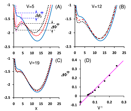
Figure 1: Stochastic bistability has a barrier height $\Delta\Phi^{{\ddagger}}(V)$ which decreases with increading $V$, as revealed by the van’t Hoff-Arrhenius analysis $\Delta\Phi^{{\ddagger}}=\Delta\phi_{0}^{{\ddagger}}+V^{-1}\Delta\phi_{1}^{{\ddagger}}$. (A-C): Blue solid line: $\phi_{0}(x)$ where $x=n/V$ is concentration of $X$ in (9); Black dots: exact $\Phi(x,V)$; Red dashed line: $\phi_{0}(x)+V^{-1}\phi_{1}(x)$ according to Eqs.(11,12) with $\theta=0.25,\nu=1.2,\gamma=15$, and different $V$s shown in the figures. (D) van’t Hoff-Arrhenius plot, with filled squares for $\Delta\Phi^{{\ddagger}}(V)$, shows a slope $\sim\Delta\phi_{1}^{{\ddagger}}>0$ and an interaction $\sim\Delta\phi_{0}^{{\ddagger}}<0$.

The ghost of extinction—A canonical phosphorylation-dephosphorylation signaling with positive feedbacks exhibits stochastic bistability bishop_qian_bj_10 :

$$E+K+E^{*}\mathop{\rightleftharpoons}^{\alpha_{1}}_{\alpha_{2}}2E^{*}+K,\ \ E^{*}+P\mathop{\rightleftharpoons}^{\beta_{1}}_{\beta_{2}}E+P,$$ (14)

in which $K$ is a kinase that catalyzes the phosphorylation reaction $E\rightarrow E^{*}$, and $P$ is a phosphatase that catalyzes the dephosphorylation reaction. The $K$ is only active, however, after binding an $E^{*}$ footnote_2 . The rates of the DGP are

$$u_{n}=\frac{k_{1}n(N-n)}{V}+k_{-2}(N-n),w_{n}=\frac{k_{-1}n(n-1)}{V}+k_{2}n,$$ (15)

where $k_{1}=\alpha_{1}[K]$, $k_{-1}=\alpha_{2}[K]$, $k_{2}=\beta_{1}[P]$, $k_{-2}=\beta_{2}[P]$ and $N$ is the total copy number of $E$ and $E^{*}$ molecules together. We have $\mu_{0}(z)=(k_{1}z+k_{-2})(e_{t}-z)$, $\mu_{1}(z)=0$, $\lambda_{0}(z)=k_{-1}z^{2}+k_{2}z$, and $\lambda_{1}(z)=-k_{-1}z$, where $e_{t}=N/V$. Therefore,

$$\phi_{0}(x) = \frac{\theta x+\nu\gamma}{\theta}\ln\left(\frac{\theta}{\nu\gamma}x+1\right)+x\ln x$$

$$- \frac{\theta x+\nu}{\theta}\ln(\theta x+\nu)+(e_{t}-x)\ln(e_{t}-x),$$

$$\phi_{1}(x) = \frac{1}{2}\ln\left[\frac{x(\theta x+\nu)(e_{t}-x)}{\theta x+\nu\gamma}\right],$$ (17)

in which $\theta,\nu,\gamma$ are again given in Eq. (13).

The stochastic bistability in (9) and Fig. 1 occurs when the system is near its deterministic bistable regime. Therefore, one can consider the stochastic bistability as a “ghost” of the saddle-node bifurcation strogatz . In the present case, $\phi_{0}(x)$ in Eq. (van’t Hoff-Arrhenius Analysis of Mesoscopic and Macroscopic Dynamics of Simple Biochemical Systems: Stochastic vs. Nonlinear Bistabilities) is a convex function with a single minimum on $[0,e_{t}]$ for all parameters. Therefore, the deterministic dynamics of (14) can not have bistability or bifurcation. It however, can have a unstable fixed point at $x=0$ when $\beta_{2}=0$. This is the case of “extinction”. Even though the $x=0$ is unstable to the ODE, the stationary distribution for the CME is $p_{n}^{st}=\delta_{n0}$: The stochastic dynamics goes extinct with probability 1. As a “ghost” of the extinction, this system can also exhibit stochastic bistability if $\beta_{2}$ is nonzero but sufficiently small bishop_qian_bj_10 . Fig. 2 shows that while $\phi_{0}(x)$ is convex. However, for finite $V$ there is a stochastic stable state at $x=0$.

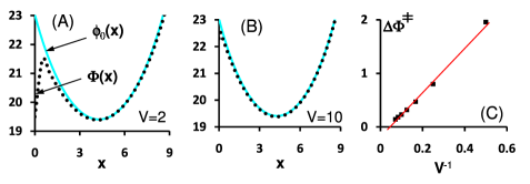
Figure 2: Solid blue lines show $\phi_{0}(x)$ according to Eq. (van’t Hoff-Arrhenius Analysis of Mesoscopic and Macroscopic Dynamics of Simple Biochemical Systems: Stochastic vs. Nonlinear Bistabilities). Black dots are $\Phi(x,V)$ following Eq. (5). Parameters used are $\theta=0.7,\nu=0.001,\gamma=1000,e_{t}=10$, with (A) $V=2$ and (B) $V=10$. $x=0$ is a stochatic stable state which disappears in the deterministic limit. (C) van’t Hoff-Arrhenius plot with filled squares for $\Delta\Phi^{{\ddagger}}$ showing a negative $\Delta\phi_{0}^{{\ddagger}}$, as expected for stochastic bistability.

System with single molecules and stochastic bistability—We have so far assumed that each term in the rates $u_{n}(V)$ and $w_{n}(V)$ corresponds to a term in $\mu_{0}(x)$ and $\lambda_{0}(x)$. However, if a chemical reaction system at finite volume contains a term $O(1)$, then in the limit of $V^{-1}u_{Vx}(V)\sim\mu_{0}(x)+V^{-1}\mu_{1}(x)+\cdots$, the term only contributes to $\mu_{1}(x)$. This is in fact the so-called “single-molecule effect”. wolynes

DGP with Lewis’ chemical detailed balance— For chemical system with a single dynamical species, the DGP predicts that chemical equilibrium has either a binomial distribution (canonical ensemble) or Poisson distribution (grand canonical ensemble) following G.N. Lewis’ principle of chemical detailed balance lewis .

The canonical ensemble has $u_{n}=k_{+}(N-n),w_{n}=k_{-}n$ ($n\leq N$), $\phi_{0}(x)=x\ln(k_{-}x/k_{+})+(e_{t}-x)\ln(e_{t}-x)$, and $\phi_{1}(x)=\frac{1}{2}\ln(x(e_{t}-x))$, with $x\leq e_{t}=N/V$. $\phi_{0}(x)$ is convex with a minimum at $\hat{x}=k_{+}e_{t}/(k_{+}+k_{-})$. More importantly, $V\phi_{0}(x)+\phi_{1}(x)$ is convex for $x\in\left(\frac{1}{2V},e_{t}-\frac{1}{2V}\right)$. Note that the asymptotic expansion $\psi(x,V)=\phi_{1}(x)+O\left(V^{-1}\right)$ is not uniformly valid at $x=0,e_{t}$. The existence of the ghost of extinction can not be determined by $\phi_{1}(x)$.

The grand canonical ensemble has $u_{n}=jV,w_{n}=kn$, $\phi_{0}(x)=x\ln(x/x^{*})-x$, and $\phi_{1}(x)=\frac{1}{2}\ln x$, where $x^{*}=j/k$. Again, convex $\phi_{0}(x)$ has a minimum at $x^{*}$, and $\phi_{1}(x)$ is concave. Still $V\phi_{0}(x)+\phi_{1}(x)$ is convex when $\left(\frac{1}{2V},\infty\right)$.

Therefore, with detailed balance in a chemical reaction system, the equilibrium distribution is always unimodal. The $\gamma$ parameter in the previous sections represents the energy dissipation of open chemical systems. One can verify that when $\gamma=1$, the results in the previous two sections are reduced to what we have here.

Exit rate of a stochastic stable state—So far we have exclusively discussed the stationary distribution in the form of $e^{-V\Phi(x,V)}$ and its relation to the stochastic bistability. We now establish the relation between the transition rate from one stable state to another and the function $\Phi(x,V)$. In a 1d birth-and-death process, the mean time of the first arrival at $n^{*}_{2}$ starting at $n^{*}_{1}$, with reflection at $0$ ($0<n_{1}^{*}<n_{2}^{*}$), has been widely used in the various lattice hopping models vanKampen :

$$T_{n_{1}^{*}\rightarrow n_{2}^{*}}=\sum_{m=n_{1}^{*}+1}^{n_{2}^{*}}\sum_{n=0}^{m-1}\frac{p^{st}_{n}(V)}{w_{m}(V)p^{st}_{m}(V)}$$ (18)

in which $p^{st}_{n}$ is the stationary distribution to Eq. (3). Let $n_{1}^{*}=Vx_{1}^{*},n_{2}^{*}=Vx_{2}^{*}$, then we found the asymptotic expansion formula $T_{x_{1}^{*}\rightarrow x_{2}^{*}}=$

$$V\int_{x_{1}^{*}}^{x_{2}^{*}}\frac{1}{\Lambda(x)}e^{V\widetilde{\Phi}(x,V)}dx\int_{0}^{x}e^{-V\widetilde{\Phi}(z,V)}dz\left[1+O\left(\frac{1}{V}\right)\right],$$ (19)

in which, the modified $\widetilde{\Phi}(x,V)=$

$$\phi_{0}(x)+\frac{1}{V}\left\{\phi_{1}(x)+\ln\frac{\mu_{0}(x)/\lambda_{0}(x)-1}{\ln(\mu_{0}(x)/\lambda_{0}(x))}\right\},$$ (20)

and $\Lambda(x)=$

$$\frac{1}{\mu_{0}(x)}\left(\frac{\lambda_{0}(x)-\mu_{0}(x)}{\ln\lambda_{0}(x)-\ln\mu_{0}(x)}\right)^{2}.$$ (21)

Noting $\Lambda(x)$ playing the role of diffusion coefficient. Eq. (19) is the same as Kramers’ theory for the rate of crossing a continous energy barrier located at $x^{{\ddagger}}\in(x_{1}^{*},x_{2}^{*})$ vanKampen . Applying Laplace’s method leads

$$T_{x_{1}^{*}\rightarrow x_{2}^{*}}\approx\frac{2\pi e^{V[\Phi(x^{{\ddagger}},V)-\Phi(x^{*}_{1},V)]}}{\lambda_{0}(x^{{\ddagger}})\sqrt{\phi_{0}^{{}^{\prime\prime}}(x_{1}^{*})|\phi_{0}^{{}^{\prime\prime}}(x^{{\ddagger}})|}}.$$ (22)

This simple relation between transition rate and $\Phi(x,V)$ are unique for 1-d system. While the concept we developed here will be valid in higher dimensional systems with saddle point, computation will be demanding hanggi .

Summary—Nonlinear biochemical reaction systems can have bi- or multi-stable behavior, which has implications to a wide range of biological processes such as epigenetic inheritance, cell differentiation, and cancer oncogenesis huang ; qian_reviews_11 . The nature and the existence of the multiple states are in the nonlinear biochemical reaction schemes and rates. For a traditional nonlinear bistable system in a small volume, the transition rates decreases with increasing system size. In the deterministic limit, these rates become zero. However, small systems can also exhibit bistable phenomenon which has no deterministic counter part. In the latter case, the bistability is due to the presence of “noise”, “stochasticity”, or “entropic barrier”. This class of bistable cellular systems can be quantitatively characterized by an van’t Hoff-Arrhenius like analysis on the volume dependence of the transition rate(s). With increasing volume, the barrier diminishes. Mathematically, the transition rate is related to the landscape of the stochastic dynamics, $k\propto e^{-V\Phi(x,V)}$ where $\Phi(x,V)$ can be decomposed into $\phi_{0}(x)+\phi_{1}/V$. Nonlinear bistable system has barrier $\Delta\phi_{0}^{{\ddagger}}>0$ while stochastic bistability has $\Delta\phi_{0}^{{\ddagger}}<0$ but $\Delta\phi_{1}^{{\ddagger}}>0$.

References

(1)
D.A. McQuarrie,
J. Appl. Prob.4, 413 (1967);
D.T. Gillespie, Ann. Rev. Phys. Chem.58, 35 (2007).
(2)
H. Qian and L.M. Bishop, Int. J. Mol. Sci.11, 3472 (2010);
H. Qian, J. Stat. Phys. (2011);
Nonlinearity (2011).
(3)
T.G. Kurtz, J. Appl. Prob.8, 344 (1971);
J. Keizer,
In Probability, Statistical Mechanics, and Number
Theory: A Volume Dedicated to Mark Kac,
G.-C. Rota Ed., pp. 1–23 (Academic Press, NY 1986).
(4)
F. Schlögl, Z. Physik.253, 147 (1972);
I.R. Epstein and J.A. Pojman,
An Introduction to Nonlinear Chemical Dynamics:
Oscillations, Waves, Patterns, and Chaos
(Oxford Univ. Press, U.K., 1998).
(5)
M. Vellela and H. Qian,
J. R. Soc. Interf. 6 925 (2009);
Bulle. Math. Biol. 69, 1727 (2007);
Proc. R. Soc. A. 466, 771 (2010).
(6)
M. Samoilov, S. Plyasunov and A.P. Arkin,
Proc. Natl. Acad. Sci. USA 102, 2310 (2005);
M.N. Artyomov, J. Das, M. Kardar and A.K. Chakraborty,
Proc. Natl. Acad. Sci. USA 104, 18958 (2007);
C.A. Miller and D.A. Beard,
Biophys. J. 95, 2183 (2008);
H. Qian, P.-Z. Shi and J. Xing,
Phys. Chem. Chem. Phys. 11, 4861 (2009);
M.N. Artyomov, M. Mathur, M.S. Samoilov and A.K. Chakraborty,
J. Chem. Phys. 131, 195103 (2009).
(7)
L.M. Bishop and H. Qian,
Biophys. J. 98, 1 (2010).
(8)
T.-L. To and N. Maheshri, Nature 327, 1142 (2010).
(9)
P. Hänggi, P. Talkner and M. Borkovec,
Rev. Mod. Phys. 62, 251 (1990).
(10)
G. Nicolis and J. W. Turner, Physica A 89, 245 (1977);
G. Nicolis and R. Lefever, Phys. Lett. A 62, 469 (1977);
C. Y. Mou, J. L. Luo, and G. Nicolis, J. Chem. Phys. 84, 7011
(1986).
(11)
G. Hu,
Zeit. Phys. B65, 103 (1986).
(12)
For complex reactions in condensed phase,
usually and
are not independent of . Then van’t Hoff
equation states and .
In the same spirit, one can decompose with
and . The relation
between this decomposition and the is
an elusive subject in classical thermodynamics. See
H.T. Benzinger, Nature, 229, 100 (1971);
H. Qian and J.J. Hopfield, J. Chem. Phys. 105, 9292 (1996);
P.W. Chun, Biophys. J. 78, 416 (2000).
(13)
In one of the major signaling pathways, Src family
kinase (SFK) is activated by its phosphorylated substrate,
SFK-dependent receptors (SDR), via SDR binding to the
SH2 domain of SFK. See J.A. Cooper and H. Qian,
Biochem.47, 5681 (2008).
(14)
S.H. Strogatz, Nonlinear Dynamics and Chaos (Westview Press,
Boston, 1994). On p. 99, critical slowdown with a bottleneck is
explained as a remant, i.e., “ghost”, of saddle-node bifurcation.
(15)
P.G. Wolynes, In Single Molecule Spectroscopy in Chemistry,
Physics and Biology,
A. Gräslund, R. Rigler and J. Widengren, eds. pp. 553–560
(Springer, New York, 2010).
(16)
G.N. Lewis,
Proc. Natl. Acad. Sci. USA11, 179 (1925).
Lewis’ detailed balance for chemical
reaction systems was formulated not
in terms of Markov processes but rather
on macroscopic LMA.
Applying his principle to the multi-dimensional
DGP, it has been shown mathematically that
the resulting stationary distribution
is a combination of multi-Poissonian
and multinomial, with its unique peak located
at the fixed point of the nonlinear ODE.
See Appendix of vellela_qian_jrsi_09
and C.W. Gardiner,
Handbook of Stochastic Methods for Physics,
Chemistry, and the Natural Sciences, 2nd Ed.,
p. 263 (Springer, New York, 1985).
(17)
N.G. van Kampen,
Stochastic Processes in Physics and
Chemistry
(Elsevier Science, North-Holland, 1992).
(18)
M. Sasai and P.G. Wolynes,
Proc. Natl. Acad. Sci. USA100, 2374 (2002);
S. Huang, G. Eichler, Y. Bar-Yam and D. Ingber,
Phys. Rev. Lett.94, 128701 (2005);
J. Wang, L. Xu, E.K. Wang and S. Huang,
Biophys. J.99, 29 (2010).