Kernel density estimation via diffusion

Abstract

We present a new adaptive kernel density estimator based on linear diffusion processes. The proposed estimator builds on existing ideas for adaptive smoothing by incorporating information from a pilot density estimate. In addition, we propose a new plug-in bandwidth selection method that is free from the arbitrary normal reference rules used by existing methods. We present simulation examples in which the proposed approach outperforms existing methods in terms of accuracy and reliability.

, and

t1Supported by Australian Research Council Grant DP0985177.

1 Introduction

Nonparametric density estimation is an important tool in the statistical analysis of data. A nonparametric estimate can be used, for example, to assess the multimodality, skewness, or any other structure in the distribution of the data Scott , Silverman . It can also be used for the summarization of Bayesian posteriors, classification and discriminant analysis Simonoff . Nonparametric density estimation has even proved useful in Monte Carlo computational methods, such as the smoothed bootstrap method and the particle filter method doufregor01 . Nonparametric density estimation is an alternative to the parametric approach, in which one specifies a model up to a small number of parameters and then estimates the parameters via the likelihood principle. The advantage of the nonparametric approach is that it offers a far greater flexibility in modeling a given dataset and, unlike the classical approach, is not affected by specification bias lehmann90 . Currently, the most popular nonparametric approach to density estimation is kernel density estimation (see Scott , Simonoff , WandJones ).

Despite the vast body of literature on the subject, there are still many contentious issues regarding the implementation and practical performance of kernel density estimators. First, the most popular data-driven bandwidth selection technique, the plug-in method sheather96 , sheather91 , is adversely affected by the so-called normal reference rule devroye97 , jones96 , which is essentially a construction of a preliminary normal model of the data upon which the performance of the bandwidth selection method depends. Although plug-in estimators perform well when the normality assumption holds approximately, at a conceptual level the use of the normal reference rule invalidates the original motivation for applying a nonparametric method in the first place.

Second, the popular Gaussian kernel density estimator MarronWand lacks local adaptivity, and this often results in a large sensitivity to outliers, the presence of spurious bumps, and in an overall unsatisfactory bias performance—a tendency to flatten the peaks and valleys of the density TerrelScott .

Third, most kernel estimators suffer from boundary bias when, for example, the data is nonnegative—a phenomenon due to the fact that most kernels do not take into account specific knowledge about the domain of the data marron94 , park03 .

These problems have been alleviated to a certain degree by the introduction of more sophisticated kernels than the simple Gaussian kernel. Higher-order kernels have been used as a way to improve local adaptivity and reduce bias jones97 , but these have the disadvantages of not giving proper nonnegative density estimates, and of requiring a large sample size for good performance MarronWand . The lack of local adaptivity has been addressed by the introduction of adaptive kernel estimators abramson , hall90 , hall95 , jones94 . These include the balloon estimators, nearest neighbor estimators and variable bandwidth kernel estimators loftsgaarden , TerrelScott , none of which yield bona fide densities, and thus remain somewhat unsatisfactory. Other proposals such as the sample point adaptive estimators are computationally burdensome (the fast Fourier transform cannot be applied Silverman ), and in some cases do not integrate to unity park03 . The boundary kernel estimators jones93 , which are specifically designed to deal with boundary bias, are either not adaptive away from the boundaries or do not result in bona fide densities foster . Thus, the literature abounds with partial solutions that obscure a unified comprehensive framework for the resolution of these problems.

The aim of this paper is to introduce an adaptive kernel density estimation method based on the smoothing properties of linear diffusion processes. The key idea is to view the kernel from which the estimator is constructed as the transition density of a diffusion process. We utilize the most general linear diffusion process that has a given limiting and stationary probability density. This stationary density is selected to be either a pilot density estimate or a density that the statistician believes represents the information about the data prior to observing the available empirical data. The approach leads to a simple and intuitive kernel estimator with substantially reduced asymptotic bias and mean square error. The proposed estimator deals well with boundary bias and, unlike other proposals, is always a bona fide probability density function. We show that the proposed approach brings under a single framework some well-known bias reduction methods, such as the Abramson estimator abramson and other variable location or scale estimators choi , hall02 , Samiuddin , jones94 .

In addition, the paper introduces an improved plug-in bandwidth selection method that completely avoids the normal reference rules jones96 that have adversely affected the performance of plug-in methods. The new plug-in method is thus genuinely “nonparametric,” since it does not require a preliminary normal model for the data. Moreover, our plug-in approach does not involve numerical optimization and is not much slower than computing a normal reference rule Matlab .

The rest of the paper is organized as follows. First, we describe the Gaussian kernel density estimator and explain how it can be viewed as a special case of smoothing using a diffusion process. The Gaussian kernel density estimator is then used to motivate the most general linear diffusion that will have a set of essential smoothing properties. We analyze the asymptotic properties of the resulting estimator and explain how to compute the asymptotically optimal plug-in bandwidth. Finally, the practical benefits of the model are demonstrated through simulation examples on some well-known datasets MarronWand . Our findings demonstrate an improved bias performance and low computational cost, and a boundary bias improvement.

2 Background

Given $N$ independent realizations $\mathcal{X}_{N}\equiv\{X_{1},\ldots,X_{N}\}$ from an unknown continuous probability density function (p.d.f.) $f$ on $\mathscr{X}$, the Gaussian kernel density estimator is defined as

$$\hat{f}(x;t)=\frac{1}{N}\sum_{i=1}^{N}\phi(x,X_{i};t),\qquad x\in\mathbb{R},$$ (1)

where

$$\phi(x,X_{i};t)=\frac{1}{\sqrt{2\pi t}}{e}^{-{(x-X_{i})^{2}}/({2t})}$$

is a Gaussian p.d.f. (kernel) with location $X_{i}$ and scale $\sqrt{t}$. The scale is usually referred to as the bandwidth. Much research has been focused on the optimal choice of $t$ in (1), because the performance of $\hat{f}$ as an estimator of $f$ depends crucially on its value sheather96 , sheather91 . A well-studied criterion used to determine an optimal $t$ is the Mean Integrated Squared Error (MISE),

$$\operatorname{MISE}\{\hat{f}\}(t)=\mathbb{E}_{f}\int[\hat{f}(x;t)-f(x)]^{2}\,dx,$$

which is conveniently decomposed into integrated squared bias and integrated variance components:

$$\operatorname{MISE}\{\hat{f}\}(t)=\int\bigl{(}\underbrace{\mathbb{E}_{f}[\hat{f}(x;t)]-f(x)}_{\mathrm{pointwise}\ \mathrm{bias}\ \mathrm{of}\ f}\bigr{)}^{2}\,dx+\int\underbrace{\operatorname{Var}_{f}[\hat{f}(x;t)]}_{\mathrm{pointwise}\ \mathrm{variance}\ \mathrm{of}\ f}dx.$$

Note that the expectation and variance operators apply to the random sample $\mathcal{X}_{N}$. The MISE depends on the bandwidth $\sqrt{t}$ and $f$ in a quite complicated way. The analysis is simplified when one considers the asymptotic approximation to the MISE, denoted AMISE, under the consistency requirements that $t=t_{N}$ depends on the sample size $N$ such that $t_{N}\downarrow 0$ and $N\sqrt{t_{N}}\rightarrow\infty$ as $N\rightarrow\infty$, and $f$ is twice continuously differentiable sheather91 . The asymptotically optimal bandwidth is then the minimizer of the AMISE. The asymptotic properties of (1) under these assumptions are summarized in Appendix A.

A key observation about the Gaussian kernel density estimator (1) is that it is the unique solution to the diffusion partial differential equation (PDE)

$$\frac{\partial}{\partial t}\hat{f}(x;t)=\frac{1}{2}\,\frac{\partial^{2}}{\partial x^{2}}\hat{f}(x;t),\qquad x\in\mathscr{X},t>0,$$ (2)

with $\mathscr{X}\equiv\mathbb{R}$ and initial condition $\hat{f}(x;0)=\Delta(x),$ where $\Delta(x)=\frac{1}{N}\sum_{i=1}^{N}\delta(x-X_{i})$ is the empirical density of the data $\mathcal{X}_{N}$ [here $\delta(x-X_{i})$ is the Dirac measure at $X_{i}$]. Equation (2) is the well-known Fourier heat equation LarssonThomee . This link between the Gaussian kernel density estimator and the Fourier heat equation has been noted in Chaudhuri and Marron chaudhuri . We will, however, go much further in exploiting this link. In the heat equation interpretation, the Gaussian kernel in (1) is the so-called Green’s function LarssonThomee for the diffusion PDE (2). Thus, the Gaussian kernel density estimator $\hat{f}(x;t)$ can be obtained by evolving the solution of the parabolic PDE (2) up to time $t$.

To illustrate the advantage of the PDE formulation over the more traditional formulation (1), consider the case where the domain of the data is known to be $\mathscr{X}\equiv[0,1]$. It is difficult to see how (1) can be easily modified to account for the finite support of the unknown density. Yet, within the PDE framework, all we have to do is solve the diffusion equation (2) over the finite domain $[0,1]$ with initial condition $\Delta(x)$ and the Neumann boundary condition

$$\frac{\partial}{\partial x}\hat{f}(x;t)\Big{|}_{x=1}=\frac{\partial}{\partial x}\hat{f}(x;t)\Big{|}_{x=0}=0.$$

The boundary condition ensures that $\frac{d}{dt}\int_{\mathscr{X}}\hat{f}(x;t)\,dx=0$, from where it follows that $\int_{\mathscr{X}}\hat{f}(x;t)\,dx=\int_{\mathscr{X}}\hat{f}(x;0)\,dx=1$ for all $t\geq 0$. The analytical solution of this PDE in this case is bellman

$$\hat{f}(x;t)=\frac{1}{N}\sum_{i=1}^{N}\kappa(x,X_{i};t),\qquad x\in[0,1],$$ (3)

where the kernel $\kappa$ is given by

$$\quad\kappa(x,X_{i};t)=\sum_{k=-\infty}^{\infty}\phi(x,2k+X_{i};t)+\phi(x,2k-X_{i};t),\qquad x\in[0,1].$$ (4)

Thus, the kernel accounts for the boundaries in a manner similar to the boundary correction of the reflection method Silverman . We now compare the properties of the kernel (4) with the properties of the Gaussian kernel $\phi$ in (1).

First, the series representation (4) is useful for deriving the small bandwidth properties of the estimator in (3). The asymptotic behavior of $\kappa(x,X_{i};t)$ as $t\rightarrow 0$ in the interior of the domain $[0,1]$ is no different from that of the Gaussian kernel, namely,

$$\sum_{k=-\infty}^{\infty}\phi(x,2k+X_{i};t)+\phi(x,2k-X_{i};t)\sim\phi(x,X_{i};t),\qquad t\downarrow 0,$$

for any fixed $x$ in the interior of the domain $[0,1]$. Here $q(t)\sim z(t),t\downarrow t_{0}$ stands for $\lim_{t\downarrow t_{0}}\frac{q(t)}{z(t)}=1$. Thus, for small $t$, the estimator (3) behaves like the Gaussian kernel density estimator (1) in the interior of $[0,1]$. Near the boundaries at $x=0,1$, however, the estimator (3) is consistent, while the Gaussian kernel density estimator is inconsistent. In particular, a general result in Appendix D includes as a special case the following boundary property of the estimator (3):

$$\mathbb{E}_{f}\hat{f}(x_{N};t_{N})=f(x_{N})+O\bigl{(}\sqrt{t_{N}}\bigr{)},\qquad N\rightarrow\infty,$$

where $x_{N}=\alpha t_{N}$ for some $\alpha\in[0,1]$, and $t_{N}\downarrow 0$ as $N\rightarrow\infty$. This shows that (3) is consistent at the boundary $x=0$. Similarly, (3) can be shown to be consistent at the boundary $x=1$. In contrast, the Gaussian kernel density estimator (1) is inconsistent WandJones in the sense that

$$\mathbb{E}_{f}\hat{f}(0;t_{N})=\tfrac{1}{2}f(0)+O\bigl{(}\sqrt{t_{N}}\bigr{)},\qquad N\rightarrow\infty.$$

The large bandwidth behavior ($t\rightarrow\infty$) of (3) is obtained from the following equivalent expression for (4) (see bellman ):

$$\kappa(x,X_{i};t)=\sum_{k=-\infty}^{\infty}{e}^{-k^{2}\pi^{2}t/2}\cos(k\pi x)\cos(k\pi X_{i}).$$ (5)

From (5), we immediately see that

$$\kappa(x,X_{i};t)\sim 1+2{e}^{-\pi^{2}t/2}\cos(\pi x)\cos(\pi X_{i}),\qquad t\rightarrow\infty,x\in[0,1].$$ (6)

In other words, as the bandwidth becomes larger and larger, the kernel (4) approaches the uniform density on $[0,1]$.

Remark 1.

An important property of the estimator (3) is that the number of local maxima or modes is a nonincreasing function of $t$. This follows from the maximum principle for parabolic PDE; see, for example, LarssonThomee .

For example, a necessary condition for a local maximum at, say, $(x_{0},t_{0}),t_{0}>0,x_{0}\in(0,1)$ is $\frac{\partial^{2}}{\partial x^{2}}\hat{f}(x_{0};t_{0})\leq 0$. From (2), this implies $\frac{\partial}{\partial t}\hat{f}(x_{0};t_{0})\leq 0$, from which it follows that there exists an $\varepsilon>0$ such that $\hat{f}(x_{0};t_{0})\geq\hat{f}(x_{0};t_{0}+\varepsilon)$. As a consequence of this, as $t$ becomes larger and larger, the number of local maxima of (3) is a nonincreasing function. This property is shared by the Gaussian kernel density estimator (1) and has been exploited in various ways by Silverman Silverman .

Example 1.

Figure 1 gives an illustration of the performance of estimators (3) and (1), where the true p.d.f. is the beta density $4(1-x)^{3},x\in[0,1]$, and the estimators are build from a

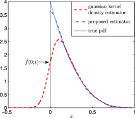
Figure 1: Boundary bias in the neighborhood of $x=0$.

sample of size $N=1000$ with a common bandwidth $\sqrt{t}=0.05248$. Note that the Gaussian kernel density estimator is close to half the value of the true p.d.f. at the boundary $x=0$. Overall, the diffusion estimator (3) is much closer to the true p.d.f. The proposed estimator (3) appears to be the first kernel estimator that does not use boundary transformation and yet is consistent at all boundaries and remains a genuine p.d.f. (is nonnegative and integrates to one). Existing boundary correction methods HallPark02 , Alberts , Karunamuni either account for the bias at a single end-point, or the resulting estimators are not genuine p.d.f.’s.

Remark 2.

In applications such as the smoothed bootstrap doufregor01 , there is a need for efficient random variable generation from the kernel density estimate. Generation of random variables from the kernel (4) is easily accomplished using the following procedure. Generate $Z\sim\mathsf{N}(0,t)$ and let $Y=X_{i}+Z$. Compute $W=Y\operatorname{mod}2$, and let $X=|W|$. Then it is easy to show (e.g., using characteristic functions) that $X$ has the density given by (4).

Given the nice boundary bias properties of the estimator that arises as the solution of the diffusion PDE (2), it is of interest to investigate if equation (2) can be somehow modified or generalized to arrive at an even better kernel estimator. This motivates us to consider in the next section the most general linear time-homogeneous diffusion PDE as a starting point for the construction of a better kernel density estimator.

3 The diffusion estimator

Our extension of the simple diffusion model (2) is based on the smoothing properties of the linear diffusion PDE

$$\frac{\partial}{\partial t}g(x;t)=Lg(x;t),\qquad x\in\mathscr{X},t>0,$$ (7)

where the linear differential operator $L$ is of the form $\frac{1}{2}\frac{d}{dx}(a(x)\frac{d}{dx}(\frac{\cdot}{p(x)}))$, and $a$ and $p$ can be any arbitrary positive functions on $\mathscr{X}$ with bounded second derivatives, and the initial condition is $g(x,0)=\Delta(x)$. If the set $\mathscr{X}$ is bounded, we add the boundary condition $\frac{\partial}{\partial x}(\frac{g(x;t)}{p(x)})=0$ on $\partial\mathscr{X}$, which ensures that the solution of (7) integrates to unity. The PDE (7) describes the p.d.f. of $X_{t}$ for the Itô diffusion process $(X_{t},t>0)$ given by ethier

$$dX_{t}=\mu(X_{t})\,dt+\sigma(X_{t})\,dB_{t},$$ (8)

where the drift coefficient $\mu(x)=\frac{a^{\prime}(x)}{2p(x)}$, the diffusion coefficient $\sigma(x)=\sqrt{\frac{a(x)}{p(x)}}$, the initial state $X_{0}$ has distribution $\Delta(x)$, and $(B_{t},t>0)$ is standard Brownian motion. Obviously, if $a=1$ and $p=1$, we revert to the simpler model (2). What makes the solution $g(x;t)$ to (7) a plausible kernel density estimator is that $g(x;t)$ is a p.d.f. with the following properties. First, $g(\cdot;0)$ is identical to the initial condition of (7), that is, to the empirical density $\Delta(x)$. This property is possessed by both the Gaussian kernel density estimator (1) and the diffusion estimator (3). Second, if $p(x)$ is a p.d.f. on $\mathscr{X}$, then

$$\lim_{t\rightarrow\infty}g(x;t)=p(x),\qquad x\in\mathscr{X}.$$

This property is similar to the property that the kernel (6) and the estimator (3) converge to the uniform density on $\mathscr{X}\equiv[0,1]$ as $t\rightarrow\infty$. In the context of the diffusion process governed by (8), $p$ is the limiting and stationary density of the diffusion. Third, similar to the estimator (3) and the Gaussian kernel density estimator (1), we can write the solution of (7) as

$$g(x;t)=\frac{1}{N}\sum_{i=1}^{N}\kappa(x,X_{i};t),$$ (9)

where for each fixed $y\in\mathscr{X}$ the diffusion kernel $\kappa$ satisfies the PDE

$$\cases{\dfrac{\partial}{\partial t}\kappa(x,y;t)=L\kappa(x,y;t),&\quad$x\in\mathscr{X},t>0$,\vspace*{2pt}\cr\kappa(x,y;0)=\delta(x-y),&\quad$x\in\mathscr{X}$.}$$ (10)

In addition, for each fixed $x\in\mathscr{X}$ the kernel $\kappa$ satisfies the PDE

$$\cases{\dfrac{\partial}{\partial t}\kappa(x,y;t)=L^{*}\kappa(x,y;t),&\quad$y\in\mathscr{X},t>0$,\vspace*{2pt}\cr\kappa(x,y;0)=\delta(x-y),&\quad$y\in\mathscr{X}$,}$$ (11)

where $L^{*}$ is of the form $\frac{1}{2p(y)}\,\frac{\partial}{\partial y}(a(y)\frac{\partial}{\partial y}(\cdot))$; that is, $L^{*}$ is the adjoint operator of $L$. Note that $L^{*}$ is the infinitesimal generator of the Itô diffusion process in (8). If the set $\mathscr{X}$ has boundaries, we add the Neumann boundary condition

$$\frac{\partial}{\partial x}\biggl{(}\frac{\kappa(x,y;t)}{p(x)}\biggr{)}\bigg{|}_{x\in\partial\mathscr{X}}=0\qquad\forall t>0$$ (12)

and $\frac{\partial}{\partial y}\kappa(x,y;t)|_{y\in\partial\mathscr{X}}=0$ to (10) and (11), respectively. These boundary conditions ensure that $g(x;t)$ integrates to unity for all $t\geq 0$. The reason that the kernel $\kappa$ satisfies both PDEs (10) and (11) is that (10) is the Kolmogorov forward equation ethier corresponding to the diffusion process (8), and (11) is a direct consequence of the Kolmogorov backward equation. We will use the forward and backward equations to derive the asymptotic properties of the diffusion estimator (9). Before we proceed with the asymptotic analysis, we illustrate how the model (7) possesses adaptive smoothing properties similar to the ones possessed by the adaptive kernel density estimators abramson , hall90 , hall95 , jones94 .

Example 2.

Suppose that the initial condition of PDE (7) is $\Delta(x)$ with $N=500\mbox{,}000$ and $X_{1},\ldots,X_{N}$ are independent draws from $f(x)=1-\cos(6\pi x),x\in[0,1]$. Suppose further that $p(x)=4(1-x)^{3}$ and $a(x)=1$ on $[0,1]$. The aim of this example is not to estimate $f$, but to illustrate the various shapes that the estimator can take, given data from $f$. Figure 2 shows the solution of the PDE (7) for two values of the bandwidth: $\sqrt{t}=4\times 10^{-4}$ (small) and $\sqrt{t}=0.89$ (large). Since $p(x)$ is the limiting and stationary density of the

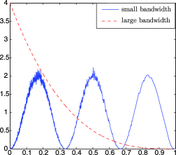
Figure 2: Small and large bandwidth behavior of the diffusion density in Example 2.

diffusion process governed by (7), the large bandwidth density is indistinguishable from $p(x)$. The small bandwidth density estimate is much closer to $f(x)$ than to $p(x)$. The crucial feature of the small bandwidth density estimate is that $p(x)$ allows for varying degrees of smoothing across the domain of the data, in particular allowing for greater smoothing to be applied in areas of sparse data, and relatively less in the high density regions. It can be seen from Figure 2 that the small time density estimate is noisier in regions where $p(x)$ is large (closer to $x=0$), and smoother in regions where $p(x)$ is small (closer to $x=1$). The adaptive smoothing is a consequence of the fact that the diffusion kernel (10) has a state-dependent diffusion coefficient $\sigma(x)=\sqrt{a(x)/p(x)}$, which helps diffuse the initial density $\Delta(x)$ at a different rate throughout the state space.

Remark 3.

Even though there is no analytical expression for the diffusion kernel satisfying (10), we can write $\kappa$ in terms of a generalized Fourier series in the case that $\mathscr{X}$ is bounded:

$$\kappa(x,y;t)=p(x)\sum_{k=0}^{\infty}{e}^{\lambda_{k}t}\varphi_{k}(x)\varphi_{k}(y),\qquad x,y\in[0,1],$$ (13)

where $\{\varphi_{k}\}$ and $\{\lambda_{k}\}$ are the eigenfunctions and eigenvalues of the Sturm–Liouville problem on $[0,1]$:

$$L^{*}\varphi_{k} = \lambda_{k}\varphi_{k},\qquad k=0,1,2,\ldots,$$

$$\varphi_{k}^{\prime}(0) = \varphi_{k}^{\prime}(1)=0,\qquad k=0,1,2,\ldots.$$

It is well known (see, e.g., LarssonThomee ) that $\{\varphi_{k}\}$ forms a complete orthonormal basis with respect to the weight $p$ for $L^{2}(0,1)$. From the expression (13), we can see that the kernel satisfies the detailed balance equation for a continuous-time Markov process ethier

$$p(y)\kappa(x,y;t)=p(x)\kappa(y,x;t)\qquad\forall t>0,x,y\in\mathscr{X}.$$ (15)

The detailed balance equation ensures that the limiting and stationary density of the diffusion estimator (9) is $p(x)$. In addition, the kernel satisfies the Chapman–Kolmogorov equation

$$\int_{\mathscr{X}}\kappa(x_{1},x_{0};t_{1})\kappa(x_{2},x_{1};t_{2})\,dx_{1}=\kappa(x_{2},x_{0};t_{1}+t_{2}).$$ (16)

Note that there is no loss of generality in assuming that the domain is $[0,1]$, because any bounded domain can be mapped onto $[0,1]$ by a linear transformation.

Remark 4.

When $p(x)$ is a p.d.f., an important distance measure between the diffusion estimator (9) and $p(x)$ is the divergence measure of Csiszár Csiszer . The Csiszár distance measure between two continuous probability densities $g$ and $p$ is defined as

$$\mathcal{D}(g\rightarrow p)=\int_{\mathbb{R}}p(x)\psi\biggl{(}\frac{g(x)}{p(x)}\biggr{)}\,dx,$$

where $\psi\dvtx\mathbb{R}_{+}\rightarrow\mathbb{R}_{+}$ is a twice continuously differentiable function; $\psi(1)=0$; and $\psi^{\prime\prime}(x)>0$ for all $x\in\mathbb{R}_{+}$. The diffusion estimator (9) possesses the monotonicity property

$$\frac{d}{dt}\mathcal{D}(g\rightarrow p)=-\frac{1}{2}\int_{\mathscr{X}}\biggl{(}\frac{g(x;t)}{p(x)}\biggr{)}^{2}\psi^{\prime\prime}\biggl{(}\frac{g(x;t)}{p(x)}\biggr{)}\,dx<0,\qquad g\not=p,t>0.$$

In other words, the distance between the estimator (9) and the stationary density $p$ is a monotonically decreasing function of the bandwidth $\sqrt{t}$. This is why the solution of (7) in Figure 2 approaches $p$ as the bandwidth becomes larger and larger. Note that Csiszár’s family of measures subsumes all of the information-theoretic distance measures used in practice Havrda-Charvat , kapkes87 . For example, if $\psi(x)=\frac{x^{\alpha}-x}{\alpha(\alpha-1)},\alpha\not=0,1$, for some parameter $\alpha$, then the family of distances indexed by $\alpha$ includes the Hellinger distance for $\alpha=1/2$, Pearson’s $\chi^{2}$ discrepancy measure for $\alpha=2$, Neymann’s $\chi^{2}$ measure for $\alpha=-1$, the Kullback–Leibler distance in the limit as $\alpha\rightarrow 1$ and Burg’s distance as $\alpha\rightarrow 0$.

4 Bias and variance analysis

We now examine the asymptotic bias, variance and MISE of the diffusion estimator (9). In order to derive the asymptotic properties of the proposed estimator, we need the small bandwidth behavior of the diffusion kernel satisfying (10). This is provided by the following lemma.

Lemma 1.

Assume that the functions $a(x)$ and $p(x)$ are such that

$$\displaystyle c_{1}=\sqrt{\int_{-\infty}^{\infty}\biggl{(}\frac{Lq(z)}{q(z)}\biggr{)}^{2}\,dz}<\infty,\qquad q(z):=\frac{p(z)}{a^{1/4}(z)p^{1/4}(z)},$$

(17)

$$\displaystyle\lim_{z\rightarrow\infty}\int_{z_{0}}^{z}\sqrt{p(s)/a(s)}\,ds=\infty.$$

Then, the leading small bandwidth asymptotic behavior of the kernel satisfying (10) and (11) on $\mathscr{X}\equiv\mathbb{R}$ is

$$\kappa(x,y;t) \sim \frac{p(x)}{\sqrt{2\pi t}[p(x)a(x)a(y)p(y)]^{1/4}}$$

$${}\times\exp\Biggl{\{}-\frac{1}{2t}\Biggl{[}\int_{y}^{x}\sqrt{\frac{p(s)}{a(s)}}\,ds\Biggr{]}^{2}\Biggr{\}},\qquad t\downarrow 0.$$

We denote the asymptotic approximation on the right-hand side by $\widetilde{\kappa}(x,y;t)$. Thus, $\kappa(x,y;t)\sim\widetilde{\kappa}(x,y;t)$ as $t\downarrow 0$.

The somewhat lengthy and technical proof is given in Appendix B. A few remarks about the technical conditions on $a$ and $p$ now follow. Conditions (1) are trivially satisfied if $a,p$ and its derivatives up to order 2 are all bounded from above, and $p(x)\geq p_{0}>0$ and $a(x)\geq a_{0}>0$. In other words, if we clip $p(x)$ away from zero and use $a(x)=p^{\alpha}(x)$ for $\alpha\in[0,1]$, then the conditions (1) are satisfied. Such clipping procedures have been applied in the traditional kernel density estimation setting, see abramson , choi , hall95 , hall02 , jones94 . Note that the conditions are more easily satisfied when $p$ is heavy-tailed. For example, if $a(x)=p(x)$, then $p$ could be any regularly varying p.d.f. of the form $p\varpropto(1+|x|)^{-\alpha},\alpha>1$. Lemma 1 is required for deriving the asymptotic properties of the estimator, all collected in the following theorem.

Theorem 1.

Let $t=t_{N}$ be such that $\lim_{N\rightarrow\infty}t_{N}=0$, $\lim_{N\rightarrow\infty}N\sqrt{t_{N}}=\infty$. Assume that $f$ is twice continuously differentiable and that the domain $\mathscr{X}\equiv\mathbb{R}$. Then:

1. The pointwise bias has the asymptotic behavior

   $$\mathbb{E}_{f}[g(x;t)]-f(x)=tLf(x)+O(t^{2}),\qquad N\rightarrow\infty.$$ (18)

2. The integrated squared bias has the asymptotic behavior

   $$\|\mathbb{E}_{f}[g(\cdot;t)]-f\|^{2}\sim t^{2}\|Lf\|^{2}=\tfrac{1}{4}t^{2}\bigl{\|}\bigl{(}a(f/p)^{\prime}\bigr{)}^{\prime}\bigr{\|}^{2},\qquad N\rightarrow\infty.$$ (19)

3. The pointwise variance has the asymptotic behavior

   $$\operatorname{Var}_{f}[g(x;t)]\sim\frac{f(x)}{2N\sqrt{\pi t}\sigma(x)},\qquad N\rightarrow\infty,$$ (20)

   where $\sigma^{2}(x)=a(x)/p(x)$.

4. The integrated variance has the asymptotic behavior

   $$\int\operatorname{Var}_{f}[g(x;t)]\,dx\sim\frac{\mathbb{E}_{f}[\sigma^{-1}(X)]}{2N\sqrt{\pi t}},\qquad N\rightarrow\infty.$$ (21)

5. Combining the leading order bias and variance terms gives the asymptotic approximation to the MISE

   $$\operatorname{AMISE}\{g\}(t)=\frac{1}{4}t^{2}\bigl{\|}\bigl{(}a(f/p)^{\prime}\bigr{)}^{\prime}\bigr{\|}^{2}+\frac{\mathbb{E}_{f}[\sigma^{-1}(X)]}{2N\sqrt{\pi t}}.$$ (22)

6. Hence, the square of the asymptotically optimal bandwidth is

   $$t^{*}=\biggl{(}\frac{\mathbb{E}_{f}[\sigma^{-1}(X)]}{2N\sqrt{\pi}\|Lf\|^{2}}\biggr{)}^{2/5},$$ (23)

   which gives the minimum

   $$\min_{t}\operatorname{AMISE}\{g\}(t)=N^{-4/5}\frac{5[\mathbb{E}_{f}\sigma^{-1}(X)]^{4/5}\|Lf\|^{2/5}}{2^{14/5}\pi^{2/5}}.$$ (24)

The proof is given in Appendix C.

We make the following observations. First, if $p\not\equiv f$, the rate of convergence of (24) is $O(N^{-4/5})$, the same as the rate of the Gaussian kernel density estimator in (39). The multiplicative constant of $N^{-4/5}$ in (24), however, can be made very small by choosing $p$ to be a pilot density estimate of $f$. Preliminary or pilot density estimates are used in most adaptive kernel methods WandJones . Second, if $p\equiv f$, then the leading bias term (18) is 0. In fact, if $f$ is infinitely smooth, the pointwise bias is exactly zero, as can be seen from

$$\mathbb{E}_{f}[g(x;t)]=\sum_{k=0}^{\infty}\frac{t^{k}}{k!}L^{k}f(x),\qquad f\in C^{\infty},$$

where $L^{n+1}=LL^{n}$ and $L^{0}$ is the identity operator. In addition, if $a=p\varpropto 1$, then the bias term (18) is equivalent to the bias term (35) of the Gaussian kernel density estimator. Third, (20) suggests that in regions where the pilot density $p(x)$ is large [which is equivalent to small diffusion coefficient $\sigma(x)$] and $f(x)$ is large, the pointwise variance will be large. Conversely, in regions with few observations [i.e., where the diffusion coefficient $\sigma(x)$ is high and $f(x)$ is small] the pointwise variance is low. In other words, the ideal variance behavior results when the diffusivity $\sigma(x)$ behaves inversely proportional to $f(x)$.

4.1 Special cases of the diffusion estimator

We shall now show that the diffusion kernel estimator (9) is a generalization of some well-known modifications of the Gaussian kernel density estimator (1). Examples of modifications and improvements subsumed as special cases of (9) are as follows.

1. If $a(x)=p(x)\varpropto 1$ in (9) and $\mathscr{X}\equiv\mathbb{R}$, then the kernel $\kappa$ reduces to the Gaussian kernel and we obtain (1).

2. If $a(x)=1$ and $p(x)=f_{p}(x)$, where $f_{p}$ is a clipped pilot density estimate of $f$ (see abramson , hall02 , jones94 ), then from Lemma 1, we have

   $$\kappa(x,y;t)\sim\widetilde{\kappa}(x,y;t)=\frac{f_{p}(x)}{\sqrt{2\pi t}(f_{p}(x)f_{p}(y))^{1/4}}\exp\biggl{\{}-\frac{1}{2t}\biggl{[}\int_{y}^{x}\sqrt{f_{p}(s)}\,ds\biggr{]}^{2}\biggr{\}}.$$

   Thus, in the neighborhood of $y$ such that $|x-y|=O(t^{\beta}),\beta>1/3$, we have

   $$\kappa(x,y;t)\sim\frac{1}{\sqrt{2\pi t/f_{p}(x)}}\exp\biggl{\{}-\frac{(x-y)^{2}}{2t/f_{p}(x)}\biggr{\}},\qquad t\downarrow 0.$$

   In other words, in the neighborhood of $y$, $\kappa$ is asymptotically equivalent to a Gaussian kernel with mean $y$ and bandwidth $\sqrt{t/f_{p}(y)}$, which is precisely the Abramson’s variable bandwidth abramson modification as applied to the Gaussian kernel. Abramson’s square root law states that the asymptotically optimal variable bandwidth is proportional to $f_{p}^{-1/2}(y)$.

3. If we choose $a(x)=p(x)=f_{p}(x)$, then in an $O(t^{\beta}),\beta>0$ neighborhood of $y$, the kernel $\kappa(x,y;t)$ behaves asymptotically as a Gaussian kernel with location $y+\frac{t}{2}\frac{f_{p}^{\prime}(y)}{f_{p}(y)}$ and bandwidth $\sqrt{t}$:

   $$\kappa(x,y;t)\sim\frac{1}{\sqrt{2\pi t}}\exp\biggl{\{}-\frac{1}{2t}\biggl{(}x-y-\frac{t}{2}\frac{f_{p}^{\prime}(y)}{f_{p}(y)}\biggr{)}^{2}\biggr{\}},\qquad t\downarrow 0.$$

   This is precisely the data sharpening modification described in Samiuddin , where the locations of the data points are shifted prior to the application of the kernel density estimate. Thus, in our paradigm, data sharpening is equivalent to using the diffusion (7) with drift $\mu(x)=\frac{f_{p}^{\prime}(x)}{2f_{p}(x)}$ and diffusion coefficient $\sigma(x)=1$.

4. Finally, if we set $p(x)=f_{p}(x)$ and $a(x)=p^{\alpha}(x)$, $\alpha\in[0,1]$, then we obtain a method that is a combination of both the data sharpening and the variable bandwidth of Abramson. The kernel $\kappa$ behaves asymptotically [in an $O(t^{\beta}),\beta>1/3$ neighborhood of $y$] like a Gaussian kernel with location $y+t\mu(y)=y+\frac{\alpha t}{2}f_{p}^{\alpha-2}(y)f_{p}^{\prime}(y)$ and bandwidth $\sqrt{t\sigma^{2}(y)}=\sqrt{tf_{p}^{\alpha-1}(y)}$. Similar variable location and scale kernel density estimators are considered in jones94 .

The proposed method thus unifies many of the already existing ideas for variable scale and location kernel density estimators. Note that these estimators all have one common feature: they compute a pilot density estimate (which is an infinite-dimensional parameter) prior to the main estimation step.

Our choice for $a(x)$ will be motivated by regularity properties of the diffusion process underlying the smoothing kernel. In short, we prefer to choose $a(x)=1$ so as to make the diffusion process in (8) nonexplosive with a well-defined limiting distribution. A necessary and sufficient condition for explosions is Feller’s test feller .

Theorem 2 ((Feller’s test)).

Let $\mu(x)>0$ and $\sigma(x)>0$ be bounded and continuous. Then the diffusion process (8) explodes if and only if there exists $z\in\mathbb{R}$ such that either one of the following two conditions holds:

1. $$\int_{-\infty}^{z}\int_{x}^{z}\exp\biggl{(}\int_{x}^{y}\frac{2\mu(s)}{\sigma^{2}(s)}\,ds\biggr{)}\sigma^{-2}(y)\,dy\,dx<\infty,$$

2. $$\int_{z}^{\infty}\int_{z}^{x}\exp\biggl{(}\int_{x}^{y}\frac{2\mu(s)}{\sigma^{2}(s)}\,ds\biggr{)}\sigma^{-2}(y)\,dy\,dx<\infty.$$

A corollary of Feller’s test is that when $\mu(x)=0$ both of Feller’s conditions fail, and diffusions of the form $dX_{t}=\sigma_{t}\,dW_{t}$ are nonexplosive.

Since in our case we have $\sigma^{2}(x)=a(x)/p(x)$ and $a(x)=\exp(\int_{x_{0}}^{x}2\mu(y)/\break\sigma^{2}(y)\,dy)$, Feller’s condition becomes the following.

Proposition 1 ((Feller’s test)).

Given $a(x)$ and $p(x)$ in (7), the diffusion process (8) explodes if and only if there exists $z\in\mathbb{R}$ such that either one of the following two conditions holds:

1. $$\int_{-\infty}^{z}\int_{x}^{z}\frac{p(y)}{a(x)}\,dy\,dx<\infty,$$

2. $$\int_{z}^{\infty}\int_{z}^{x}\frac{p(y)}{a(x)}\,dy\,dx<\infty.$$

The easiest way to ensure nonexplosiveness of the underlying diffusion process and the existence of a limiting distribution is to set $a(x)=1$, which corresponds to $\mu(x)=0$. Note that a necessary condition for the existence of a limiting p.d.f. is the existence of $z$ such that $\int_{z}^{\infty}1/a(x)\,dx=\infty$. In this case, both of Feller’s conditions fail. The nonexplosiveness property ensures that generation of random variables from the diffusion estimator does not pose any technical problems.

5 Bandwidth selection algorithm

Before we explain how to estimate the bandwidth $\sqrt{t^{*}}$ in (23) of the diffusion estimator (9), we explain how to estimate the bandwidth $\sqrt{{}_{*}t}$ in (38) (see Appendix A) of the Gaussian kernel density estimator (1). Here, we present a new plug-in bandwidth selection procedure based on the ideas in sheather96 , JonesMarronPark , Marron , sheather91 to achieve unparalleled practical performance. The highlighting feature of the proposed method is that it does not use normal reference rules and is thus completely data-driven.

It is clear from (38) in Appendix A that to compute the optimal ${}_{*}t$ for the Gaussian kernel density estimator (1) one needs to estimate the functional $\|f^{\prime\prime}\|^{2}$. Thus, we consider the problem of estimating $\|f^{(j)}\|^{2}$ for an arbitrary integer $j\geq 1$. The identity $\|f^{(j)}\|^{2}=(-1)^{j}\mathbb{E}_{f}[f^{(2j)}(X)]$ suggests two possible plug-in estimators. The first one is

$$(-1)^{j}\widehat{\mathbb{E}_{f}f^{(2j)}}:\! = \frac{(-1)^{j}}{N}\sum_{k=1}^{N}\hat{f}^{(2j)}(X_{k};t_{j})$$

$$= \frac{(-1)^{j}}{N^{2}}\sum_{k=1}^{N}\sum_{m=1}^{N}\phi^{(2j)}(X_{k},X_{m};t_{j}),$$

where $\hat{f}$ is the Gaussian kernel density estimator (1). The second estimator is

$$\bigl{\|}\widehat{f^{(j)}}\bigr{\|}^{2}:\! = \bigl{\|}\hat{f}^{(j)}(\cdot;t)\bigr{\|}^{2}$$

$$= \frac{1}{N^{2}}\sum_{k=1}^{N}\sum_{m=1}^{N}\int_{\mathbb{R}}\phi^{(j)}(x,X_{k};t_{j})\phi^{(j)}(x,X_{m};t_{j})\,dx$$

$$= \frac{(-1)^{j}}{N^{2}}\sum_{k=1}^{N}\sum_{m=1}^{N}\phi^{(2j)}(X_{k},X_{m};2t_{j}),$$

where the last line is a simplification following easily from the fact that the Gaussian kernel $\phi$ satisfies the Chapman–Kolmogorov equation (16). For a given bandwidth, both estimators $(-1)^{j}\widehat{\mathbb{E}_{f}f^{(2j)}}$ and $\widehat{\|f^{(j)}\|}{}^{2}$ aim to estimate the same quantity, namely $\|f^{(j)}\|^{2}$. We select $t_{j}$ so that both estimators (5) and (5) are asymptotically equivalent in the mean square error sense. In other words, we choose $t_{j}={{}_{*}}t_{j}$ so that both $(-1)^{j}\widehat{\mathbb{E}_{f}f^{(2j)}}$ and $\widehat{\|f^{(j)}\|}{}^{2}$ have equal asymptotic mean square error. This gives the following proposition.

Proposition 2.

The estimators $(-1)^{j}\widehat{\mathbb{E}_{f}f^{(2j)}}$ and $\widehat{\|f^{(j)}\|}{}^{2}$ have the same asymptotic mean square error when

$$_{*}t_{j}=\biggl{(}\frac{1+{1}/{2^{j+1/2}}}{3}\frac{1\times 3\times 5\times\cdots\times(2j-1)}{N\sqrt{\pi/2}\|f^{(j+1)}\|^{2}}\biggr{)}^{{2}/({3+2j})}.$$ (27)

The arguments are similar to the ones used in WandJones . Under the assumptions that $t_{j}$ depends on $N$ such that $\lim_{N\rightarrow\infty}t_{j}=0$ and$\lim_{N\rightarrow\infty}Nt_{j}^{j+1/2}=\infty$, we can take the expectation of the estimator (5) and obtain the expansion $(t_{j}=t)$:

$$\mathbb{E}_{f}\bigl{[}\widehat{\mathbb{E}_{f}f^{(2j)}}\bigr{]}$$

$$\qquad=\frac{1}{N}\phi^{(2j)}(0,0;t)+\frac{N-1}{N}\int\!\!\int f(x)f(y)\phi^{(2j)}(x,y;t)\,dx\,dy$$

$$\qquad=-\frac{1\times 3\times\cdots\times(2j-1)}{t^{j+1/2}\sqrt{2\pi}N}$$

$$\qquad\quad{}+\int f(x)\biggl{(}f^{(2j)}(x)+\frac{t}{2}f^{2(j+1)}(x)+o(t)\biggr{)}\,dx+O(N^{-1})$$

$$\qquad=-\frac{1\times 3\times 5\times\cdots\times(2j-1)}{t^{j+1/2}\sqrt{2\pi}N}+\frac{t}{2}\bigl{\|}f^{(j+1)}\bigr{\|}^{2}$$

$$\qquad\quad{}+(-1)^{j}\bigl{\|}f^{(j)}\bigr{\|}^{2}+O(N^{-1}),\qquad N\rightarrow\infty.$$

Hence, the squared bias has asymptotic behavior ($N\rightarrow\infty$)

$$\bigl{(}(-1)^{j}\mathbb{E}_{f}\bigl{[}\widehat{\mathbb{E}_{f}f^{(2j)}}\bigr{]}-\bigl{\|}f^{(j)}\bigr{\|}^{2}\bigr{)}^{2}\sim\biggl{(}\frac{1\times 3\times\cdots\times(2j-1)}{t^{j+1/2}\sqrt{2\pi}N}-\frac{t}{2}\bigl{\|}f^{(j+1)}\bigr{\|}^{2}\biggr{)}^{2}.$$

A similar argument (see WandJones ) shows that the variance is of the order $O(N^{-2}\times\break t^{-2j-1/2})$, which is of lesser order than the squared bias. This implies that the leading order term in the asymptotic mean square error of $\widehat{\mathbb{E}_{f}f^{(2j)}}$ is given by the asymptotic squared bias. There is no need to derive the asymptotic expansion of $\mathbb{E}_{f}[\widehat{\|f^{(j)}\|}{}^{2}]$, because inspection of (5) and (5) shows that $\widehat{\|f^{(j)}\|}{}^{2}$ exactly equals $(-1)^{j}\widehat{\mathbb{E}_{f}f^{(2j)}}$ when the latter is evaluated at $2t_{j}$. In other words,

$$(-1)^{j}\mathbb{E}_{f}\bigl{[}\widehat{\bigl{\|}f^{(j)}\bigr{\|}}^{2}\bigr{]} = -\frac{1\times 3\times 5\times\cdots\times(2j-1)}{(2t)^{j+1/2}\sqrt{2\pi}N}$$

$${}+t\bigl{\|}f^{(j+1)}\bigr{\|}^{2}+O(1+N^{-1}).$$

Again, the leading term of the asymptotic mean square error of $\widehat{\|f^{(j)}\|}{}^{2}$ is given by the leading term of the squared bias of $\widehat{\|f^{(j)}\|}{}^{2}$. Thus, equalizing the asymptotic mean squared error of both estimators is the same as equalizing their respective asymptotic squared biases. This yields the equation

$$\biggl{(}\frac{1\times 3\times\cdots\times(2j-1)}{(2t)^{j+1/2}\sqrt{2\pi}N}-t\bigl{\|}f^{(j+1)}\bigr{\|}^{2}\biggr{)}^{2}$$

$$\qquad=\biggl{(}\frac{1\times 3\times\cdots\times(2j-1)}{t^{j+1/2}\sqrt{2\pi}N}-\frac{t}{2}\bigl{\|}f^{(j+1)}\bigr{\|}^{2}\biggr{)}^{2}.$$

The positive solution of the equation yields the desired ${{}_{*}}t_{j}$.

Thus, for example,

$$_{*}t_{2}=\biggl{(}\frac{8+\sqrt{2}}{24}\frac{3}{N\sqrt{\pi/2}\|f^{(3)}\|^{2}}\biggr{)}^{2/7}$$ (28)

is our bandwidth choice for the estimation of $\|f^{\prime\prime}\|^{2}$. We estimate each ${}_{*}t_{j}$ by

$${{}_{*}}\hat{t}_{j}=\biggl{(}\frac{1+{1}/{2^{j+1/2}}}{3}\frac{1\times 3\times 5\times\cdots\times(2j-1)}{N\sqrt{\pi/2}\widehat{\|f^{(j+1)}\|}{}^{2}}\biggr{)}^{{2}/({3+2j})}.$$ (29)

Computation of $\widehat{\|f^{(j+1)}\|}{}^{2}$ requires estimation of ${{}_{*}}t_{j+1}$ itself, which in turn requires estimation of ${{}_{*}}t_{j+2}$, and so on, as seen from formulas (5) and (29). We are faced with the problem of estimating the infinite sequence $\{{{}_{*}}t_{j+k},k\geq 1\}$. It is clear, however, that given ${}_{*}t_{l+1}$ for some $l>0$ we can estimate all $\{_{*}t_{j},1\leq j\leq l\}$ recursively, and then estimate ${}_{*}t$ itself from (38). This motivates the $l$-stage direct plug-in bandwidth selector sheather96 , sheather91 , WandJones , defined as follows.

1. For a given integer $l>0$, estimate ${}_{*}t_{l+1}$ via (27) and $\|f^{(l+2)}\|^{2}$ computed by assuming that $f$ is a normal density with mean and variance estimated from the data. Denote the estimate by ${}_{*}\hat{t}_{l+1}$.

2. Use ${}_{*}\hat{t}_{l+1}$ to estimate $\|f^{(l+1)}\|^{2}$ via the plug-in estimator (5) and ${}_{*}\hat{t}_{l}$ via (29). Then use ${}_{*}\hat{t}_{l}$ to estimate ${}_{*}\hat{t}_{l-1}$ and so on until we obtain an estimate of ${}_{*}\hat{t}_{2}$.

3. Use the estimate of ${}_{*}\hat{t}_{2}$ to compute ${}_{*}\hat{t}$ from (38).

The $l$-stage direct plug-in bandwidth selector thus involves the estimation of $l$ functionals $\{\|f^{(j)}\|,2\leq j\leq l+1\}$ via the plug-in estimator (5). We can describe the procedure in a more abstract way as follows. Denote the functional dependence of ${}_{*}\hat{t}_{j}$ on ${}_{*}\hat{t}_{j+1}$ in formula (29) as

$${}_{*}\hat{t}_{j}=\gamma_{j}(_{*}\hat{t}_{j+1}).$$

It is then clear that ${}_{*}\hat{t}_{j}=\gamma_{j}(\gamma_{j+1}(_{*}\hat{t}_{j+2}))=\gamma_{j}(\gamma_{j+1}(\gamma_{j+2}(_{*}\hat{t}_{j+3})))=\cdots.$ For simplicity of notation, we define the composition

$$\gamma^{[k]}(t)=\underbrace{\gamma_{1}(\cdots\gamma_{k-1}(\gamma_{k}}_{k\ \mathrm{times}}(t))\cdots),\qquad k\geq 1.$$

Inspection of formulas (29) and (38) shows that the estimate of ${}_{*}t$ satisfies

$${}_{*}\hat{t} = \xi{{}_{*}}\hat{t}_{1}=\xi\gamma^{[1]}(_{*}\hat{t}_{2})=\xi\gamma^{[2]}({{}_{*}}\hat{t}_{3})=\cdots=\xi\gamma^{[l]}({{}_{*}}\hat{t}_{1+l}),$$

$$\xi = \biggl{(}\frac{6\sqrt{2}-3}{7}\biggr{)}^{2/5}\approx 0.90.$$

Then, for a given integer $l>0$, the $l$-stage direct plug-in bandwidth selector consists of computing

$${}_{*}\hat{t}=\xi\gamma^{[l]}(_{*}t_{l+1}),$$

where ${}_{*}t_{l+1}$ is estimated via (27) by assuming that $f$ in $\|f^{(l+2)}\|^{2}$ is a normal density with mean and variance estimated from the data. The weakest point of this procedure is that we assume that the true $f$ is a Gaussian density in order to compute $\|f^{(l+2)}\|^{2}$. This assumption can lead to arbitrarily bad estimates of ${}_{*}{t}$, when, for example, the true $f$ is far from being Gaussian. Instead, we propose to find a solution to the nonlinear equation

$$t=\xi\gamma^{[l]}(t),$$ (30)

for some $l$, using either fixed point iteration or Newton’s method with initial guess $t=0$. The fixed point iteration version is formalized in the following algorithm.

Algorithm 1 ((Improved Sheather–Jones)).

Given $l>2$, execute the following steps:

1. initialize with $z_{0}=\varepsilon$, where $\varepsilon$ is machine precision, and $n=0$;

2. set $z_{n+1}=\xi\gamma^{[l]}(z_{n})$;

3. if $|z_{n+1}-z_{n}|<\varepsilon$, stop and set ${}_{*}\hat{t}=z_{n+1}$; otherwise, set $n:=n+1$ and repeat from step 2;

4. deliver the Gaussian kernel density estimator (1) evaluated at ${}_{*}\hat{t}$ as the final estimator of $f$, and ${}_{*}\hat{t}_{2}=\gamma^{[l-1]}(z_{n+1})$ as the bandwidth for the optimal estimation of $\|f^{\prime\prime}\|^{2}$.

Numerical experience suggests the following. First, the fixed-point algorithm does not fail to find a root of the equation $t=\xi\gamma^{[l]}(t)$. Second, the root appears to be unique. Third, the solutions to the equations

$$t=\xi\gamma^{[5]}(t)$$

and

$$t=\xi\gamma^{[l+5]}(t)$$

for any $l>0$ do not differ in any practically meaningful way. In other words, there were no gains to be had by increasing the stages of the bandwidth selection rule beyond $l=5$. We recommend setting $l=5$. Finally, the numerical procedure for the computation of $\gamma^{[5]}(t)$ is fast when implemented using the Discrete Cosine Transform Matlab .

The plug-in method described in Algorithm 1 has superior practical performance compared to existing plug-in implementations, including the particular solve-the-equation rule of Sheather and Jones sheather91 , WandJones . Since we borrow many of the fruitful ideas described in sheather91 (which in turn build upon the work of Hall, Park and Marron hall87 , park1990 ), we call our new algorithm the Improved Sheather–Jones (ISJ) method.

To illustrate the significant improvement of the plug-in method in Algorithm 1, consider, for example, the case where $f$ is a mixture of two Gaussian densities with a common variance of $1$ and means of $-30$ and $30$.

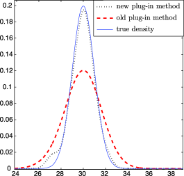
Figure 3: The Improved Sheather–Jones bandwidth selection rule in Algorithm 1 leads to improved performance compared to the original plug-in rule that uses the normal reference rule.

Figure 3 shows the right mode of $f$, and the two estimates resulting from the old plug-in rule sheather91 and the plug-in rule of Algorithm 1. The left mode is not displayed, but looks similar. The integrated squared error using the new plug-in bandwidth estimate, $\|f-\hat{f}(\cdot;{{}_{*}}\hat{t})\|^{2}$, is one 10th of the error using the old bandwidth selection rule.

5.1 Experiments with normal reference rules

The result of Figure 3 is not an isolated case, in which the normal reference rules do not perform well. We performed a comprehensive simulation study in order to compare the Improved Sheather–Jones (ISJ) (Algorithm 1) with the original (vanilla) Sheather–Jones (SJ) algorithm sheather91 , WandJones .

Table 1: Results over 10 independent simulation experiments. In all cases the domain was assumed to be $\mathbb{R}$. Many test problems are taken from MarronWand . In the table $\mathsf{N}(\mu,\sigma^{2})$, denotes a Gaussian density with mean $\mu$ and variance $\sigma^{2}$

Case	Target density $\bolds{f(x)}$	$\bolds{N}$	Ratio
1 (claw)	$\frac{1}{2}\mathsf{N}(0,1)+\sum_{k=0}^{4}\frac{1}{10}\mathsf{N}(\frac{k}{2}-1,(\frac{1}{10})^{2})$	$10^{3}$	0.72
		$10^{4}$	0.94
2 (strongly skewed)	$\sum_{k=0}^{7}\frac{1}{8}\mathsf{N}(3((\frac{2}{3})^{k}-1),(\frac{2}{3})^{2k})$	$10^{3}$	0.69
		$10^{4}$	0.84
3 (kurtotic unimodal)	$\frac{2}{3}\mathsf{N}(0,1)+\frac{1}{3}\mathsf{N}(0,(\frac{1}{10})^{2})$	$10^{2}$	0.78
		$10^{3}$	0.93
4 (double claw)	$\frac{49}{100}\mathsf{N}(-1,(\frac{2}{3})^{2})+\frac{49}{100}\mathsf{N}(1,(\frac{2}{3})^{2})$	$10^{5}$	0.35
	$+\,\frac{1}{350}\sum_{k=0}^{6}\mathsf{N}(\frac{k-3}{2},(\frac{1}{100})^{2})$	$10^{6}$	0.10
5 (discrete comb)	$\frac{2}{7}\sum_{k=0}^{2}\mathsf{N}(\frac{12k-15}{7},(\frac{2}{7})^{2})+\frac{1}{21}\sum_{k=8}^{10}\mathsf{N}(\frac{2k}{7},(\frac{1}{21})^{2})$	$10^{3}$	0.45
		$10^{4}$	0.27
6 (asymmetric	$\frac{46}{100}\sum_{k=0}^{1}\mathsf{N}(2k-1,(\frac{2}{3})^{2})+\sum_{k=1}^{3}\frac{1}{300}\mathsf{N}(-\frac{k}{2},(\frac{1}{100})^{2})$	$10^{4}$	0.68
double claw)	$+\,\sum_{k=1}^{3}\frac{7}{300}\mathsf{N}(\frac{k}{2},(\frac{7}{100})^{2})$	$10^{6}$	0.24
7 (outlier)	$\frac{1}{10}\mathsf{N}(0,1)+\frac{9}{10}\mathsf{N}(0,(\frac{1}{10})^{2})$	$10^{3}$	1.01
		$10^{5}$	1.00
8 (separated bimodal)	$\frac{1}{2}\mathsf{N}(-12,\frac{1}{4})+\frac{1}{2}\mathsf{N}(12,\frac{1}{4})$	$10^{2}$	0.33
		$10^{3}$	0.64
9 (skewed bimodal)	$\frac{3}{4}\mathsf{N}(0,1)+\frac{1}{4}\mathsf{N}(\frac{3}{2},(\frac{1}{3})^{2})$	$10^{3}$	1.02
		$10^{4}$	1.00
10 (bimodal)	$\frac{1}{2}\mathsf{N}(0,(\frac{1}{10})^{2})+\frac{1}{2}\mathsf{N}(5,1)$	$10^{2}$	0.31
		$10^{3}$	0.70
11	Log-Normal with $\mu=0$ and $\sigma=1$	$10^{3}$	0.82
		$10^{4}$	0.80
12 (asymmetric claw)	$\frac{1}{2}\mathsf{N}(0,1)+\sum_{k=-2}^{2}\frac{2^{1-k}}{31}\mathsf{N}(k+\frac{1}{2},(\frac{2^{-k}}{10})^{2})$	$10^{3}$	0.76
		$10^{4}$	0.59
13 (trimodal)	$\frac{1}{3}\sum_{k=0}^{2}\mathsf{N}(80k;(k+1)^{4})$	$10^{2}$	0.21
		$10^{3}$	0.17
14 (5-modes)	$\frac{1}{5}\sum_{k=0}^{4}\mathsf{N}(80k;(k+1)^{2})$	$10^{3}$	0.07
		$10^{4}$	0.18
15 (10-modes)	$\frac{1}{10}\sum_{k=0}^{9}\mathsf{N}(100k;(k+1)^{2})$	$10^{3}$	0.12
		$10^{4}$	0.07
16 (smooth comb)	$\sum_{k=0}^{5}\frac{2^{5-k}}{63}\mathsf{N}(\frac{65-96/2^{k}}{21};\frac{(32/63)^{2}}{2^{2k}})$	$10^{4}$	0.40
		$10^{5}$	0.34

Table 1 shows the average results over 10 independent trials for a number of different test cases. The second column displays the target density and the third column shows the sample size used for the experiments. The last column shows our criterion for comparison:

$$R=\frac{\|\hat{f}(\cdot;{{}_{*}}\hat{t})-f\|^{2}}{\|\hat{f}(\cdot;t_{\mathrm{SJ}})-f\|^{2}},$$

that is, the ratio of the integrated squared error of the new ISJ estimator to the integrated squared error of the original SJ estimator. Here, $t_{\mathrm{SJ}}$ is the bandwidth computed using the original Sheather–Jones method sheather91 , WandJones .

The results in Table 1 show that the improvement in the integrated squared error can be as much as ten-fold, and the ISJ method outperforms the SJ method in almost all cases. The evidence suggests that discarding the normal reference rules, widely employed by most plug-in rules, can significantly improve the performance of the plug-in methods.

The multi-modal test cases 12 through 16 in Table 1 and Figure 3 demonstrate that the new bandwidth selection procedure passes the bi-modality test devroye97 , which consists of testing the performance of a bandwidth selection procedure using a bimodal target density, with the two modes at some distance from each other. It has been demonstrated in devroye97 that, by separating the modes of the target density enough, existing plug-in selection procedures can be made to perform arbitrarily poorly due to the adverse effects of the normal reference rules. The proposed plug-in method in Algorithm 1 performs much better than existing plug-in rules, because it uses the theoretical ideas developed in sheather91 , except for the detrimental normal reference rules. A Matlab implementation of Algorithm 1 is freely available from Matlab , and includes other examples of improved performance.

Algorithm 1 can be extended to bandwidth selection in higher dimensions. For completeness we describe the two-dimensional version of the algorithm in Appendix E. The advantages of discarding the normal reference rules persist in the two-dimensional case. In other words, the good performance of the proposed method in two dimensions is similar to that observed in the univariate case. For example, Figure 4 shows the superior

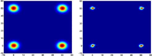
Figure 4: Right panel: plug-in rule with normal reference rule; left panel: the Improved Sheather–Jones method; the normal reference rule causes significant over-smoothing.

performance of the ISJ method compared to a plug-in approach using the normal reference rule wand94 , WandJones , and with kernels assumed to have a diagonal covariance matrix with a single smoothing parameter: $\Sigma=tI$. We estimate the bivariate density, $\frac{1}{4}\sum_{k=1}^{4}\mathsf{N}(\bolds\mu_{k},I)$, from a sample of size $N=400$, where

$$\bolds\mu_{1}=(0,0),\qquad\bolds\mu_{2}=(0,50),\qquad\bolds\mu_{3}=(50,0),\qquad\bolds\mu_{4}=(50,50).$$

Note that using a plug-in rule with a normal reference rule causes significant over-smoothing. The integrated squared error for the ISJ method is 10 times smaller than the corresponding error for the plug-in rule that uses a normal reference rule wand94 , WandJones .

5.2 Bandwidth selection for the diffusion estimator

We now discuss the bandwidth choice for the diffusion estimator (9). In the following argument we assume that $f$ is as many times continuously differentiable as needed. Computation of $t^{*}$ in (23) requires an estimate of $\|Lf\|^{2}$ and $\mathbb{E}_{f}[\sigma^{-1}(X)]$. We estimate $\mathbb{E}_{f}[\sigma^{-1}(X)]$ via the unbiased estimator $\frac{1}{N}\sum_{i=1}^{N}\sigma^{-1}(X_{i})$. The identity $\|Lf\|^{2}=\mathbb{E}_{f}L^{*}Lf(X)$ suggests two possible plug-in estimators. The first one is

$$\widehat{\mathbb{E}_{f}L^{*}Lf}:\! = \frac{1}{N}\sum_{j=1}^{N}L^{*}Lg(x;t_{2})\Big{|}_{x=X_{j}}$$

$$= \frac{1}{N^{2}}\sum_{i=1}^{N}\sum_{j=1}^{N}L^{*}L\kappa(x,X_{i};t_{2})\Big{|}_{x=X_{j}},$$

where $g(x;t_{2})$ is the diffusion estimator (9) evaluated at $t_{2}$, and $\mathscr{X}\equiv\mathbb{R}$. The second estimator is

$$\widehat{\|Lf\|}{}^{2}:\! = \|Lg(\cdot;t_{2})\|^{2}$$

$$= \biggl{\|}\frac{\partial g}{\partial t}(\cdot;t_{2})\biggr{\|}^{2}$$

$$= \frac{1}{N^{2}}\sum_{i=1}^{N}\sum_{j=1}^{N}\int_{\mathbb{R}}\,\frac{\partial\kappa}{\partial t}(x,X_{i};t_{2})\frac{\partial\kappa}{\partial t}(x,X_{j};t_{2})\,dx$$

$$= \frac{1}{N^{2}}\sum_{i=1}^{N}\sum_{j=1}^{N}L^{*}L\kappa(x,X_{i};2t_{2})\Big{|}_{x=X_{j}},$$

where the last line is a simplification that follows from the Chapman–Kolmogorov equation (16). The optimal $t^{*}_{2}$ is derived in the same way that ${}_{*}t_{2}$ is derived for the Gaussian kernel density estimator. That is, $t^{*}_{2}$ is such that both estimators $\widehat{\mathbb{E}_{f}L^{*}Lf}$ and $\widehat{\|Lf\|}{}^{2}$ have the same asymptotic mean square error. This leads to the following proposition.

Proposition 3.

The estimators $\widehat{\mathbb{E}_{f}L^{*}Lf}$ and $\widehat{\|Lf\|}{}^{2}$ have the same asymptotic mean square error when

$$t^{*}_{2}=\biggl{(}\frac{8+\sqrt{2}}{24}\frac{-3\sqrt{2}\mathbb{E}_{f}[\sigma^{-1}(X)]}{8\sqrt{\pi}N\mathbb{E}_{f}[L^{*}L^{2}f(X)]}\biggr{)}^{2/7}.$$ (33)

Although the relevant calculations are lengthier, the arguments here are exactly the same as the ones used in Proposition 1. In particular, we have the same assumptions on $t$ about its dependence on $N$. For simplicity of notation, the operators $L^{*}$ and $L$ are here assumed to apply to the first argument of the kernel $\kappa$:

$$\mathbb{E}_{f}[\widehat{\mathbb{E}_{f}L^{*}Lf}]$$

$$\qquad=\mathbb{E}_{f}\frac{1}{N^{2}}\sum_{i=1}^{N}\sum_{j=1}^{N}L^{*}L\kappa(x,X_{i};t)\Big{|}_{x=X_{j}}$$

$$\qquad=\frac{1}{N}\int f(x)L^{*}L\kappa(x,X_{i};t)\Big{|}_{X_{i}=x}\,dx$$

$$\qquad\quad{}+\frac{N-1}{N}\int\!\!\int f(y)f(x)L^{*}L\kappa(x,y;t)\,dy\,dx$$

$$\qquad=\frac{3\sqrt{2}\mathbb{E}_{f}[\sigma^{-1}(X)]}{8\sqrt{\pi}t^{5/2}N}+O(N^{-1}t^{-3/2})$$

$$\qquad\quad{}+\int\!\!\int f(y)f(x)L^{*}L\kappa(x,y;t)\,dy\,dx+O(N^{-1})$$

$$\qquad=\frac{3\sqrt{2}\mathbb{E}_{f}[\sigma^{-1}(X)]}{8\sqrt{\pi}t^{5/2}N}+\int f(y)\int L^{*}Lf(x)\kappa(x,y;t)\,dx\,dy$$

$$\qquad\quad{}+O\bigl{(}N^{-1}(1+t^{-3/2})\bigr{)}$$

$$\qquad=\frac{3\sqrt{2}\mathbb{E}_{f}[\sigma^{-1}(X)]}{8\sqrt{\pi}t^{5/2}N}+\|Lf\|^{2}+t\int f(y)L^{*}L^{2}f(y)\,dy$$

$$\qquad\quad{}+O\bigl{(}N^{-1}(1+t^{-3/2})+t^{2}\bigr{)},$$

where we have used a consequence of Lemma 1,

$$\int f(x)L^{*}L\kappa(x,X_{i};t)\Big{|}_{X_{i}=x}\,dx\sim\frac{3\sqrt{2}\mathbb{E}_{f}[\sigma^{-1}(X)]}{8\sqrt{\pi}t^{5/2}},\qquad t\downarrow 0,$$

and a consequence of the detailed balance equation (15),

$$\int L^{*}Lf(x)\kappa(x,y;t)\,dx = \int\frac{p(x)L^{*}Lf(x)}{p(y)}\kappa(y,x;t)\,dx$$

$$= L^{*}Lf(y)+tL^{*}L^{*}Lf(y)+O(t^{2}).$$

Therefore, the squared bias has asymptotic behavior ($N\rightarrow\infty$)

$$(\mathbb{E}_{f}[\widehat{\mathbb{E}_{f}L^{*}Lf}]-\|Lf\|^{2})^{2}\sim\biggl{(}\frac{3\sqrt{2}\mathbb{E}_{f}[\sigma^{-1}(X)]}{8\sqrt{\pi}t^{5/2}N}+t\int f(y)L^{*}L^{2}f(y)\,dy\biggr{)}^{2}.$$

Since estimator $\widehat{\|Lf\|}{}^{2}$ equals $\widehat{\mathbb{E}_{f}L^{*}Lf}$ when the latter is evaluated at $2t_{2}$, the asymptotic squared bias of $\widehat{\|Lf\|}{}^{2}$ follows immediately, and we simply repeat the arguments in the proof of Proposition 1 to obtain the desired $t^{*}_{2}$.

Note that $t^{*}_{2}$ has the same rate of convergence to $0$ as ${{}_{*}}t_{2}$ in (28). In fact, since the Gaussian kernel density estimator is a special case of the diffusion estimator (9) when $p(x)=a(x)=1$, the plug-in estimator (5.2) for the estimation of $\|Lf\|^{2}$ reduces to the plug-in estimator for the estimation of $\frac{1}{4}\|f^{\prime\prime}\|^{2}$. In addition, when $p(x)=a(x)=1$, the $t_{2}^{*}$ in (33) and ${{}_{*}}t_{2}$ in (28) are identical. We thus suggest the following bandwidth selection and estimation procedure for the diffusion estimator (9).

Algorithm 2.

1. Given the data $X_{1},\ldots,X_{N}$, run Algorithm 1 to obtain the Gaussian kernel density estimator (1) evaluated at ${}_{*}\hat{t}$ and the optimal bandwidth $\sqrt{{{}_{*}}\hat{t}_{2}}$ for the estimation of $\|f^{\prime\prime}\|^{2}$. This is the pilot estimation step.

2. Let $p(x)$ be the Gaussian kernel density estimator from step 1, and let $a(x)=p^{\alpha}(x)$ for some $\alpha\in[0,1]$.

3. Estimate $\|Lf\|^{2}$ via the plug-in estimator (5.2) using $\hat{t}_{2}^{*}={{}_{*}}\hat{t}_{2}$, where ${{}_{*}}\hat{t}_{2}$ is computed in step 1.

4. Substitute the estimate of $\|Lf\|^{2}$ into (23) to obtain an estimate for $t^{*}$.

5. Deliver the diffusion estimator (9) evaluated at $\hat{t}^{*}$ as the final density estimate.

The bandwidth selection rule that we use for the diffusion estimator in Algorithm 2 is a single stage direct plug-in bandwidth selector, where the bandwidth $t^{*}_{2}$ for the estimation of the functional $\|Lf\|^{2}$ is approximated by ${}_{*}\hat{t}_{2}$ (which is computed in Algorithm 1), instead of being derived from a normal reference rule. In the next section, we illustrate the performance of Algorithm 2 using some well-known test cases for density estimation.

Remark 5 ((Random variable generation)).

For applications of kernel density estimation, such as the smoothed bootstrap, efficient random variable generation from the diffusion estimator (9) is accomplished via the Euler method as applied to the stochastic differential equation (8) (see Kloeden ).

Algorithm 3.

1. Subdivide the interval $[0,\hat{t}^{*}]$ into $n$ equal intervals of length $\delta t=\hat{t}^{*}/n$ for some large $n$.

2. Generate a random integer $I$ from $1$ to $N$ uniformly.

3. For $i=1,\ldots,n$, repeat

   $$Y_{i}=Y_{i-1}+\mu(Y_{i-1})\delta t+\sigma(Y_{i-1})\sqrt{\delta t}Z_{i},$$

   where $Z_{1},\ldots,Z_{n}\sim_{\mathrm{i.i.d.}}\mathsf{N}(0,1)$, and $Y_{0}=X_{I}$.

4. Output $Y_{n}$ as a random variable with approximate density (9).

Note that since we are only interested in the approximation of the statistical properties of $Y_{n}$, there are no gains to be had from using the more complex Milstein stochastic integration procedure Kloeden .

6 Numerical experiments

In this section, we provide a simulation study of the diffusion estimator. In implementing Algorithm 2, there are a number of issues to consider. First, the numerical solution of the PDE (7) is a straightforward application of either finite difference or spectral methods LarssonThomee . A Matlab implementation using finite differences and the stiff ODE solver ode15s.m is available from the first author upon request. Second, we compute $\|Lg(\cdot;\hat{t}_{2}^{*})\|^{2}$ in Algorithm 2 using the approximation

$$\|Lg(\cdot;t)\|^{2}=\biggl{\|}\frac{\partial g}{\partial t}(\cdot;t)\biggr{\|}^{2}\approx\|g(\cdot;t+\varepsilon)-g(\cdot;t)\|^{2}/\varepsilon^{2},\qquad\varepsilon\ll 1,$$

where $g(\cdot;t)$ and $g(\cdot;t+\varepsilon)$ are the successive output of the numerical integration routine (ode15s.m in our case). Finally, we selected $\alpha=1$ or $a(x)=p(x)$ in Algorithm 2 without using any clipping of the pilot estimate. For a small simulation study with $\alpha=0$, see preprint .

We would like to point out that simulation studies of existing variable-location scale estimators jones94 , Samiuddin , TerrelScott are implemented assuming that the target p.d.f. $f$ and any functionals of $f$ are known exactly and no pilot estimation step is employed. In addition, in these simulation studies the bandwidth is chosen so that it is the global minimizer of the exact MISE. Since in practical applications the MISE and all functionals of $f$ are not available, but have to be estimated, we proceed differently in our simulation study. We compare the estimator of Algorithm 2 with the Abramson’s popular adaptive kernel density estimator abramson . The parameters ${}_{*}t$ and ${}_{*}t_{2}$ of the diffusion estimator are estimated using the new bandwidth selection procedure in Algorithm 1. The implementation of Abramson’s estimator in the Stata language is given in stata . Briefly, the estimator is given by

$$\hat{f}_{\mathsf{A}}(x)=\frac{1}{N\sqrt{t}\lambda_{i}}\sum_{i=1}^{N}\phi\biggl{(}\frac{x-X_{i}}{\sqrt{t}\lambda_{i}}\biggr{)},$$

where $\lambda_{i}^{2}=G/\hat{f}(X_{i};t_{p})$, $G=(\prod_{i=1}^{N}\hat{f}(X_{i};t_{p}))^{1/N}$, and the bandwidths $\sqrt{t}$ and $\sqrt{t_{p}}$ are computed using Least Squares Cross Validation (LSCV) Loader .

Our criterion for the comparison is the numerical approximation to

$$\operatorname{Ratio}=\frac{\|g(\cdot;\hat{t}^{*})-f\|^{2}}{\|\hat{f}_{\mathsf{A}}-f\|^{2}},$$

that is, the ratio of the integrated squared error of the diffusion estimator to the integrated squared error of the alternative kernel density estimator.

Table 2: Results over 10 independent simulation experiments. In all cases the domain was assumed to be $\mathbb{R}$

Case	Target density $\bolds{f(x)}$	$\bolds{N}$	Ratio I	Ratio II
1	$\frac{1}{2}\mathsf{N}(0,(\frac{1}{10})^{2})+\frac{1}{2}\mathsf{N}(5,1)$	$10^{3}$	0.9	0.82
		$10^{5}$	0.23	0.48
2	$\frac{1}{2}\mathsf{N}(0,1)+\sum_{k=0}^{4}\frac{1}{10}\mathsf{N}(\frac{k}{2}-1,(\frac{1}{10})^{2})$	$10^{3}$	0.65	0.99
		$3\times 10^{5}$	0.11	0.51
3	$\sum_{k=0}^{7}\frac{1}{8}\mathsf{N}(3((\frac{2}{3})^{k}-1),(\frac{2}{3})^{2k})$	$10^{3}$	1.05	0.75
		$10^{5}$	0.15	0.45
4	$\frac{49}{100}\mathsf{N}(-1,(\frac{2}{3})^{2})+\frac{49}{100}\mathsf{N}(1,(\frac{2}{3})^{2})+\frac{1}{350}\sum_{k=0}^{6}\mathsf{N}(\frac{k-3}{2},(\frac{1}{100})^{2})$	$10^{3}$	0.94	0.63
		$10^{5}$	0.46	0.76
5	$\frac{2}{7}\sum_{k=0}^{2}\mathsf{N}(\frac{12k-15}{7},(\frac{2}{7})^{2})+\frac{1}{21}\sum_{k=8}^{10}\mathsf{N}(\frac{2k}{7},(\frac{1}{21})^{2})$	$10^{3}$	0.54	2.24
		$10^{5}$	0.12	0.84
6	$\frac{46}{100}\sum_{k=0}^{1}\mathsf{N}(2k-1,(\frac{2}{3})^{2})+\sum_{k=1}^{3}\frac{1}{300}\mathsf{N}(-\frac{k}{2},(\frac{1}{100})^{2})$	$10^{4}$	0.83	0.93
	$\,+\sum_{k=1}^{3}\frac{7}{300}\mathsf{N}(\frac{k}{2},(\frac{7}{100})^{2})$	$10^{5}$	0.55	0.68
7	$\frac{1}{2}\mathsf{N}(-2,\frac{1}{4})+\frac{1}{2}\mathsf{N}(2,\frac{1}{4})$	$10^{3}$	0.51	0.51
		$10^{5}$	0.41	0.89
8	$\frac{3}{4}\mathsf{N}(0,1)+\frac{1}{4}\mathsf{N}(\frac{3}{2},(\frac{1}{3})^{2})$	$10^{3}$	0.59	0.53
		$10^{6}$	0.79	1.01
9	Log-Normal with $\mu=0$ and $\sigma=1$	$10^{3}$	0.17	0.85
		$10^{5}$	0.12	0.51
10	$\frac{1}{2}\mathsf{N}(0,1)+\sum_{k=-2}^{2}\frac{2^{1-k}}{31}\mathsf{N}(k+\frac{1}{2},(\frac{2^{-k}}{10})^{2})$	$10^{3}$	0.88	0.98
		$10^{4}$	0.30	0.85

Table 2, column 4 (ratio I) shows the average results over 10 independent trials for a number of different test cases. The second column displays the target density and the third column shows the sample size used for the experiments. In the table $\mathsf{N}(\mu,\sigma^{2})$, denotes a Gaussian density with mean $\mu$ and variance $\sigma^{2}$. Most test problems are taken from MarronWand . For each test case, we conducted a simulation run with both a relatively small sample size and a relatively large sample size wherever possible. The table shows that, unlike the standard variable location-scale estimators jones94 , TerrelScott , the diffusion estimator does not require any clipping procedures in order to retain its good performance for large sample sizes.

Next, we compare the practical performance of the proposed diffusion estimator with the performance of higher-order kernel estimators. We consider the sinc kernel estimator defined as

$$\hat{f}_{\mathsf{sinc}}(x)=\frac{1}{N}\sum_{i=1}^{N}\frac{1}{\sqrt{t}}K\biggl{(}\frac{x-X_{i}}{\sqrt{t}}\biggr{)},\qquad K(x)=\frac{\sin(x)}{\pi x},$$

where again $\sqrt{t}$ is selected using LSCV. Table 2, column 5 (ratio II) shows that the results are broadly similar and our method is favored in all cases except test case 5. Higher-order kernels do not yield proper density estimators, because the kernels take on negative values. Thus, an important advantage of our method and all second order kernel methods is that they provide nonnegative density estimators. As pointed out in WandJones , the good asymptotic performance of higher-order kernels is not guaranteed to carry over to finite sample sizes in practice. Our results confirm this observation.

Table 3: Practical performance of the boundary bias correction of the diffusion estimator for the test cases: (1) exponential distribution with mean equal to unity; (2) test cases 1 through 8, truncated to the interval $(-\infty,0]$

Test case	$\bolds{\mathsf{Exp}(1)}$	1	2	3	4	5	6	7	8
Ratio	0.52	0.38	0.74	0.25	0.70	0.38	0.74	0.56	0.46

In addition, we make a comparison with the novel polynomial boundary correction method of Hall and Park hallpark . The results are given in Table 3, where we use some of the test cases defined in Table 1, truncated to the interval $(-\infty,0]$. Table 3 shows that for finite sample sizes the practical performance of our approach is competitive. We now give the implementation details. Let $\beta$ be the point of truncation from above, which is assumed to be known in advance. Then, the Hall and Park estimator is

$$\qquad\hat{f}_{\alpha}(x;t)=\frac{1}{N\int_{-\infty}^{\beta}\phi((x-y)/h)\,dy}\sum_{i=1}^{N}\phi\biggl{(}\frac{x-X_{i}+\alpha(x)}{\sqrt{t}}\biggr{)},\qquad x\leq\beta,$$ (34)

where $\alpha(x)=t\frac{\hat{f}^{\prime}_{0}(x)}{\hat{f}_{0}(x)}\rho(\frac{x-a}{h});$ $\hat{f}_{0}(x)$ is equivalent to $\hat{f}_{\alpha}(x)$ when $\alpha(x)\equiv 0$, and $\hat{f}^{\prime}_{0}(x)$ is an estimator of $f^{\prime}(x)$; $\rho(u)=\frac{1}{\phi(u)}\int_{-\infty}^{u}v\phi(v)\,dv$. We use LSCV to select a suitable bandwidth $\sqrt{t}$. The denominator in (34) adjusts for the deficit of probability mass in the neighborhood of the end-point, but note that theoretically (34) does not integrate to unity and therefore random variable generation from (34) is not straightforward. In addition, our estimator more easily handles the case with two end-points. On the positive side, Hall and Park hallpark note that their estimator preserves positivity and has excellent asymptotic properties, which is an advantage over many other boundary kernels.

Finally, we give a two-dimensional density estimation example, which to the best of our knowledge cannot be handled satisfactorily by existing methods HallPark02 , Alberts due to the boundary bias effects.

Figure 5: A two-dimensional example with 600 points generated uniformly within an ellipse.

The two-dimensional version of equation (2) is

$$\frac{\partial\hat{f}}{\partial t}(\mathbf{x};t) = \frac{1}{2}\biggl{(}\frac{\partial^{2}\hat{f}}{\partial x_{1}^{2}}(\mathbf{x};t)+\frac{\partial^{2}\hat{f}}{\partial x_{2}^{2}}(\mathbf{x};t)\biggr{)}\qquad\forall t>0,\mathbf{x}\in\mathscr{X},$$

$$\hat{f}(\mathbf{x};0) = \Delta(\mathbf{x}),$$

$$\mathbf{n}\cdot\nabla\hat{f}(\mathbf{x};t) = 0\qquad\forall t>0,$$

where $\mathbf{x}=(x_{1},x_{2})$ belongs to the set $\mathscr{X}\subseteq\mathbb{R}^{2}$, the initial condition $\Delta(\mathbf{x})$ is the empirical density of the data, and in the Neumann boundary condition $\mathbf{n}$ denotes the unit outward normal to the boundary $\partial\mathscr{X}$ at $\mathbf{x}$. The particular example which we consider is the density estimation of $600$ uniformly distributed points on the domain $\mathscr{X}=\{\mathbf{x}\dvtx x_{1}^{2}+(4x_{2})^{2}\leq 4\}$. We assume that the domain of the data $\mathscr{X}$ is known prior to the estimation. Figure 5 shows $\hat{f}(\mathbf{x};\hat{t}^{*})$ on $\mathscr{X}=\{\mathbf{x}\dvtx x_{1}^{2}+(4x_{2})^{2}\leq 4\}$, that is, it shows the numerical solution of the two-dimensional PDE at time $\hat{t}^{*}=0.13$ on the set $\mathscr{X}$. The bandwidth was determined using the bandwidth selection procedure described in Appendix E. We emphasize the satisfactory way in which the p.d.f. $\hat{f}(\mathbf{x};\hat{t}^{*})$ handles any boundary bias problems. It appears that currently existing methods HallPark02 , foster , Alberts , Karunamuni cannot handle such two-dimensional (boundary) density estimation problems either because the geometry of the set $\mathscr{X}$ is too complex, or because the resulting estimator is not a bona-fide p.d.f.

7 Conclusions and future research

We have presented a new kernel density estimator based on a linear diffusion process. The key idea is to construct an adaptive kernel by considering the most general linear diffusion with its stationary density equal to a pilot density estimate. The resulting diffusion estimator unifies many of the existing ideas about adaptive smoothing. In addition, the estimator is consistent at boundaries. Numerical experiments suggest good practical performance. As future research, the proposed estimator can be extended in a number of ways. First, we can construct kernel density estimators based on Lévy processes, which will have the diffusion estimator as a special case. The kernels constructed via a Lévy process could be tailored for data for which smoothing with the Gaussian kernel density estimator or diffusion estimator is not optimal. Such cases arise when the data is a sample from a heavy-tailed distribution. Second, more subtle and interesting smoothing models can be constructed by considering nonlinear parabolic PDEs. One such candidate is the quasilinear parabolic PDE with diffusivity that depends on the density exponentially:

$$\frac{\partial}{\partial t}g(x;t)=\frac{\partial}{\partial x}\biggl{(}{e}^{-\alpha g(x;t)}\,\frac{\partial}{\partial x}g(x;t)\biggr{)},\qquad\alpha>0.$$

Another viable model is the semilinear parabolic PDE

$$\frac{\partial}{\partial t}\bigl{(}{e}^{u(x;t)}\bigr{)}=\frac{1}{2}\,\frac{\partial^{2}}{\partial x^{2}}u(x;t),$$

where $u(x;t)=\log(g(x;t))$ is the logarithm of the density estimator. The Cauchy density $\frac{t}{\pi(x^{2}+t^{2})}$ is a particular solution and thus the model could be useful for smoothing heavy-tailed data. All such nonlinear models will provide adaptive smoothing without the need for a pilot run, but at the cost of increased model complexity.

Appendix A Gaussian kernel density estimator properties

In this appendix, we present the technical details for the proofs of the properties of the diffusion estimator. In addition, we include a description of our plug-in rule in two dimensions.

We use $\|\cdot\|$ to denote the Euclidean norm on $\mathbb{R}$.

Theorem 3.

Let $t=t_{N}$ be such that $\lim_{N\rightarrow\infty}t_{N}=0$ and $\lim_{N\rightarrow\infty}N\sqrt{t_{N}}=\infty$. Assume that $f^{\prime\prime}$ is a continuous square-integrable function. The integrated squared bias and integrated variance of the Gaussian kernel density estimator (1) have asymptotic behavior

$$\|\mathbb{E}_{f}[\hat{f}(\cdot;t)]-f\|^{2}=\tfrac{1}{4}t^{2}\|f^{\prime\prime}\|^{2}+o(t^{2}),\qquad N\rightarrow\infty,$$ (35)

and

$$\int\operatorname{Var}_{f}[\hat{f}(x;t)]\,dx=\frac{1}{2N\sqrt{\pi t}}+o\bigl{(}\bigl{(}N\sqrt{t}\bigr{)}^{-1}\bigr{)},\qquad N\rightarrow\infty,$$ (36)

respectively. The first-order asymptotic approximation of MISE, denoted AMISE, is thus given by

$$\operatorname{AMISE}\{\hat{f}\}(t)=\frac{1}{4}t^{2}\|f^{\prime\prime}\|^{2}+\frac{1}{2N\sqrt{\pi t}}.$$ (37)

The asymptotically optimal value of $t$ is the minimizer of the AMISE

$$_{*}t=\biggl{(}\frac{1}{2N\sqrt{\pi}\|f^{\prime\prime}\|^{2}}\biggr{)}^{2/5},$$ (38)

giving the minimum value

$$\operatorname{AMISE}\{\hat{f}\}(_{*}t)=N^{-4/5}\frac{5\|f^{\prime\prime}\|^{2/5}}{4^{7/5}\pi^{2/5}}.$$ (39)

For a simple proof, see WandJones .

Appendix B Proof of Lemma 1

We seek to establish the behavior of the solution of (11) and (10) as $t\downarrow 0$. We use the Wentzel–Kramers–Brillouin–Jeffreys (WKBJ) method described in azencott , Cohen , kannai , molchanov . In the WKBJ method, we look for an asymptotic expansion of the form

$$\kappa(x,y;t)\sim{e}^{-{1}/({2t})s^{2}(x,y)}\sum_{m=0}^{\infty}t^{m-1/2}C_{m}(x,y),\qquad t\downarrow 0,$$ (40)

where $\{C_{m}(x,y)\}$ and $s(x,y)$ are unknown functions. To determine $s(x,y)$ and $\{C_{m}(x,y)\}$, we substitute the expansion into (10) and, after canceling the exponential term, equate coefficients of like powers of $t$. This matching of the powers of $t$ leads to solvable ODEs, which determine the unknown functions. Eliminating the leading order $O(t^{-5/2})$ term gives the ODE for $s$

$$a(x)\biggl{[}\frac{\partial}{\partial x}s(x,y)\biggr{]}^{2}-p(x)=0.$$ (41)

Setting the next highest order $O(t^{-3/2})$ term in the expansion to zero gives the ODE

$$\qquad 0 = 2a(x)s(x,y)\,{\frac{\partial s}{\partial x}}\,{\frac{dp}{dx}}p(x)C_{0}(x,y)-2a(x)s(x,y)\,{\frac{\partial s}{\partial x}}p^{2}(x)\,{\frac{\partial C_{0}}{\partial x}}$$

$${}+p^{3}(x)C_{0}(x,y)+s^{2}(x,y)p^{3}(x)C_{1}(x,y)$$

$${}-{\frac{da}{dx}}p^{2}(x)s(x,y)\,{\frac{\partial s}{\partial x}}C_{0}(x,y)$$

$${}+a(x)s^{2}(x,y)\biggl{(}{\frac{\partial s}{\partial x}}\biggr{)}^{2}p^{2}(x)C_{1}(x,y)-a(x)\biggl{(}{\frac{\partial s}{\partial x}}\biggr{)}^{2}p^{2}(x)C_{0}(x,y)$$

$${}-a(x)s(x,y)\,{\frac{\partial^{2}s}{\partial{x}^{2}}}p^{2}(x)C_{0}(x,y).$$

To determine a unique solution to (41), we impose the condition $s(x,x)=0$, which is necessary, but not sufficient, to ensure that $\lim_{t\downarrow 0}\kappa(x,y;t)=\delta(x-y)$. This gives the solution

$$s(x,y)=\int_{y}^{x}\sqrt{\frac{p(s)}{a(s)}}\,ds.$$

Substituting this solution into (B) and simplifying gives an equation without $C_{1}(x,y)$,

$$C_{0}(x,y)p(x)\,\frac{da}{dx}+4a(x)p(x)\,\frac{\partial C_{0}}{\partial x}-3C_{0}(x,y)\,\frac{dp}{dx}a(x)=0,$$ (43)

whence we have the general solution $C_{0}(x,y)=h(y)p^{3/4}(x)a^{-1/4}(x)$ for some as yet unknown function of $y$, $h(y)$. To determine $h(y)$, we require that the kernel $\widetilde{\kappa}(x,y;t)$ satisfies the detailed balance equation (15). This ensures that $\widetilde{\kappa}(x,y;t)$ also satisfies (11). It follows that $C_{0}(x,y)$ has to satisfy $p(y)C_{0}(x,y)=p(x)C_{0}(y,x)$, which after rearranging gives

$$h(x)(a(x)p(x))^{1/4}=h(y)(a(y)p(y))^{1/4}.$$

A separation of variables argument now gives $h(y)(a(y)p(y))^{1/4}=\mathrm{const}.$, and hence

$$C_{0}(x,y)=\mathrm{const.}(a(y)p(y))^{-1/4}p^{3/4}(x)a^{-1/4}(x).$$

We still need to determine the arbitrary constant. The constant is chosen so that

$$\lim_{t\downarrow 0}\int_{-\infty}^{\infty}\widetilde{\kappa}(x,y;t)\,dx=1,$$

which ensures that $\lim_{t\downarrow 0}\widetilde{\kappa}(x,y;t)=\delta(x-y)$. This final condition yields

$$C_{0}(x,y)=\frac{p(x)}{\sqrt{2\pi}(a(y)p(y)a(x)p(x))^{1/4}},$$

and hence

$$\widetilde{\kappa}(x,y;t)=\frac{p(x)}{\sqrt{2\pi t}[p(x)a(x)a(y)p(y)]^{1/4}}\exp\Biggl{\{}-\frac{1}{2t}\Biggl{[}\int_{y}^{x}\sqrt{\frac{p(s)}{a(s)}}\,ds\Biggr{]}^{2}\Biggr{\}}.$$

Remark 6.

Matching higher powers of $t$ gives first order linear ODEs for the rest of the unknown functions $\{C_{m}(x,y),m\geq 1\}$. The ODE for each $C_{m}(x,y),m=1,2,3,\ldots$ is

$$as^{\prime}(C_{m}/p)^{\prime}+\biggl{(}\frac{(as^{\prime})^{\prime}}{2p}+(m-1/2)\biggr{)}C_{m}=\bigl{(}a(C_{m-1}/p)^{\prime}\bigr{)}^{\prime},\qquad C_{m}(y,y)=0,$$

where all derivatives apply to the variable $x$ and $y$ is treated as a constant. Thus, in principle, all functions $\{C_{m}(x,y)\}$ can be uniquely determined.

It can be shown (see Cohen ) that the expansion (40) is valid under the conditions that $a,p$ and all their derivatives are bounded from above, and $p(x)\geq p_{0}>0$, $a(x)\geq a_{0}>0$. Here, we only establish the validity of the leading order approximation $\widetilde{\kappa}$ under the milder conditions (1). We do not attempt to prove the validity of the higher order terms in (40) under the weaker conditions. The proof of the following lemma uses arguments similar to the ones given in Cohen .

Lemma 2.

Let $a(x)$ and $p(x)$ satisfy conditions (1). Then, for all $t\in(0,t_{0}]$, where $t_{0}>0$ is some constant independent of $x$ and $y$, there holds

$$|\kappa(x,y;t)-\widetilde{\kappa}(x,y;t)|\leq\operatorname{const.}C_{0}(x,y)t^{1/4}{e}^{-{s^{2}(x,y)}/({2t})}\qquad\forall x,y.$$

To prove the lemma, we first begin by proving the following auxiliary results.

Proposition 4.

Define

$$\ell(z)=\ell(z;x,y,t,\tau)=\frac{s^{2}(x,z)}{2(t-\tau)}+\frac{s^{2}(z,y)}{2\tau}.$$

Then for $\tau\in(0,t)$, we have

$$\ell(z)\geq\frac{s^{2}(x,y)}{2t}.$$

Moreover, there exists a unique $z_{0}=z_{0}(x,y,t,\tau)$ for which $\ell(z_{0})=\frac{s^{2}(x,y)}{2t}$, and $\ell(z)$ is increasing for $z>z_{0}$ and decreasing for $z<z_{0}$.

We have

$$\ell(z)=\frac{1}{2(t-\tau)}\biggl{(}\int_{z}^{x}\sigma^{-1}(s)\,ds\biggr{)}^{2}+\frac{1}{2\tau}\biggl{(}\int_{y}^{z}\sigma^{-1}(s)\,ds\biggr{)}^{2},$$

and hence

$$\ell^{\prime}(z)=\frac{-\sigma^{-1}(z)}{t-\tau}\int_{z}^{x}\sigma^{-1}(s)\,ds+\frac{\sigma^{-1}(z)}{\tau}\int_{y}^{z}\sigma^{-1}(s)\,ds.$$ (44)

For $x\not=y$, $\ell^{\prime}(y)>0,\ell^{\prime}(x)<0$, and therefore by the continuity of $\ell^{\prime}$, there exists $z_{0}\in(x,y)\dvtx\ell^{\prime}(z_{0})=0$. For $x=y$, set $z_{0}=x$. Setting $z=z_{0}$ in (44),

$$\frac{1}{t-\tau}\int_{z_{0}}^{x}\sigma^{-1}(s)\,ds=\frac{1}{\tau}\int_{y}^{z_{0}}\sigma^{-1}(s)\,ds.$$ (45)

Therefore, ${\int_{z_{0}}^{x}}\sigma^{-1}(s)\,ds=\frac{t-\tau}{\tau}{\int_{y}^{z_{0}}}\sigma^{-1}(s)\,ds$ and adding ${\int_{y}^{z_{0}}}\sigma^{-1}(s)\,ds$ to both sides we obtain

$$\int_{y}^{x}\sigma^{-1}(s)\,ds=\frac{t}{\tau}\int_{y}^{z_{0}}\sigma^{-1}(s)\,ds,$$

from which we see that (45) is also equal to $\frac{1}{t}{\int_{y}^{x}}\sigma^{-1}(s)\,ds$. Hence, by substitution $\ell(z_{0})=\frac{1}{2t}(\int_{y}^{x}\sigma^{-1}(s)\,ds)^{2}$, as required. Finally, note that if $F(z)=\ell(z)-\frac{t}{2\tau(t-\tau)}(\int_{z_{0}}^{z}\sigma^{-1}(s)\,ds)^{2}$, then $F^{\prime}(z)=0$ for all $z$. Hence, $F(z)=F(z_{0})=\ell(z_{0})$ and

$$\ell(z)=\ell(z_{0})+\frac{t}{2\tau(t-\tau)}\biggl{(}\int_{z_{0}}^{z}\sigma^{-1}(s)\,ds\biggr{)}^{2}.$$ (46)

As a consequence of Proposition 4, we have the following result.

Proposition 5.

Assuming $\lim_{z\rightarrow\pm\infty}\int_{z_{0}}^{z}\sigma^{-1}(s)\,ds=\pm\infty$, we have the following equality:

$$\int_{0}^{t}\sqrt{\int_{-\infty}^{\infty}\biggl{(}\frac{{e}^{-{s^{2}(x,z)}/({2(t-\tau)})}}{\sqrt{t-\tau}}\frac{{e}^{-{s^{2}(z,y)}/({2\tau})}}{\sqrt{\sigma(z)}\sqrt{\tau}}\biggr{)}^{2}\,dz}\,d\tau$$

$$\qquad=2\pi^{-1/4}t^{1/4}\Gamma^{2}(3/4){e}^{-{s^{2}(x,y)}/({2t})}$$

$$\qquad=c_{2}t^{1/4}{e}^{-{s^{2}(x,y)}/({2t})},$$

where $c_{2}$ is a constant [indeed $c_{2}=2\pi^{-1/4}\Gamma^{2}(3/4)$].

We have

$$\int_{-\infty}^{\infty}\frac{{e}^{-{s^{2}(x,z)}/{(t-\tau)}}}{t-\tau}\frac{{e}^{-{s^{2}(z,y)}/{\tau}}}{\sigma(z)\tau}\,dz$$

$$\qquad=\frac{1}{(t-\tau)\tau}{e}^{-2\ell(z_{0})}\int_{-\infty}^{\infty}\sigma^{-1}(z){e}^{-{(\int_{z_{0}}^{z}\sigma^{-1}(s)\,ds)^{2}}/({\tau(t-\tau)/t})}\,dz$$

$$\qquad=\frac{1}{\sqrt{t(t-\tau)\tau}}{e}^{-2\ell(z_{0})}\int_{-\infty}^{\infty}{e}^{-v^{2}}\,dv,$$

with the change of variable $v(z)=\frac{1}{\sqrt{\tau(t-\tau)/t}}\int_{z_{0}}^{z}\sigma^{-1}(s)\,ds$. Then the result follows from the fact that $\int_{0}^{t}(\tau(t-\tau))^{-1/4}\,d\tau=2\pi^{-1/2}t^{1/2}\Gamma^{2}(3/4)$.

Given these two auxiliary results, we proceed with the proof of Lemma 2. Writing

$$\kappa^{*}(x,y;t)=\frac{\partial}{\partial t}\widetilde{\kappa}(x,y;t)-L\widetilde{\kappa}(x,y;t)=-\frac{{e}^{-{s^{2}(x,y)}/({2t})}}{\sqrt{t}}LC_{0}(x,y),$$

we define inductively the following sequence of function $\{\rho_{j}\}$, starting with $\rho_{0}=0$:

$$\rho_{j+1}(x,y;t) = -\kappa^{*}(x,y;t)-\int_{0}^{t}\int_{-\infty}^{\infty}\kappa^{*}(x,z;t-\tau)\rho_{j}(z,y;\tau)\,dz\,d\tau,$$

$$\eqntext{j=1,2,\ldots.}$$ (47)

Note in particular that $\rho_{1}=-\kappa^{*}$. We will show that there exists a limit of $\{\rho_{j}\}$. We begin by proving via induction that for $j\geq 1$, $x,y\in\mathbb{R}$, $t\in(0,t_{0}]$, where

$$t_{0}=\min\biggl{\{}\biggl{(}\frac{\sqrt{2\pi}}{2c_{1}c_{2}}\biggr{)}^{4/3},1\biggr{\}},$$

there holds

$$|\rho_{j+1}(x,y,t)-\rho_{j}(x,y,t)|\leq\frac{c_{3}}{2^{j}}|LC_{0}(x,y)|t^{1/4}{e}^{-{s^{2}(x,y)}/({2t})},$$ (48)

where $c_{3}=2c_{1}c_{2}/\sqrt{2\pi}$. First, we calculate for $j=1$

$$\rho_{2}(x,y,t)=-\kappa^{*}(x,y,t)+\int_{0}^{t}\int_{-\infty}^{\infty}\kappa^{*}(x,z,t-\tau)\kappa^{*}(z,y,\tau)\,dz\,d\tau.$$

Therefore, we have the following bound:

$$|\rho_{2}(x,y,t)-\rho_{1}(x,y,t)|$$

$$\qquad\leq\int_{0}^{t}\int_{-\infty}^{\infty}|\kappa^{*}(x,z,t-\tau)\kappa^{*}(z,y,\tau)|\,dz\,d\tau$$

$$\qquad=\int_{0}^{t}\int_{-\infty}^{\infty}\frac{{e}^{-{s^{2}(x,z)}/({2(t-\tau)})}}{\sqrt{t-\tau}}\frac{{e}^{-{s^{2}(z,y)}/({2\tau})}}{\sqrt{\tau}}|LC_{0}(x,z)LC_{0}(z,y)|\,dz\,d\tau$$

$$\qquad=\int_{0}^{t}\int_{-\infty}^{\infty}\frac{{e}^{-{s^{2}(x,z)}/({2(t-\tau)})}}{\sqrt{t-\tau}}\frac{{e}^{-{s^{2}(z,y)}/({2\tau})}}{\sqrt{\sigma(z)\tau}}$$

$$\qquad\quad\hskip 34.8pt{}\times\sqrt{\sigma(z)}|LC_{0}(x,y)|\frac{|Lq(z)|}{\sqrt{2\pi}(a(z)p(z))^{1/4}}\,dz\,d\tau$$

$$\qquad=\frac{1}{\sqrt{2\pi}}|LC_{0}(x,y)|\int_{0}^{t}\int_{-\infty}^{\infty}\frac{{e}^{-{s^{2}(x,z)}/({2(t-\tau)})}}{\sqrt{t-\tau}}$$

$$\qquad\quad\hskip 113.6pt{}\times\frac{{e}^{-{s^{2}(z,y)}/({2\tau})}}{\sqrt{\sigma(z)\tau}}\frac{|Lq(z)|}{q(z)}\,dz\,d\tau$$

$$\qquad\leq\frac{1}{\sqrt{2\pi}}|LC_{0}(x,y)|c_{1}c_{2}t^{1/4}{e}^{-{s^{2}(x,y)}/({2t})},$$

where the last inequality follows from the Cauchy–Schwarz inequality, Proposition 5 and assumption (1). We thus have

$$|\rho_{2}(x,y,t)-\rho_{1}(x,y,t)|\leq\frac{c_{3}}{2}|LC_{0}(x,y)|t^{1/4}{e}^{-{s^{2}(x,y)}/({2t})}.$$

Next, assume the induction statement is true for $2,3,\ldots,j-1$. Then

$$|\rho_{j+1}(x,y,t)-\rho_{j}(x,y,t)|$$

$$\qquad\leq\int_{0}^{t}\int_{-\infty}^{\infty}|\kappa^{*}(x,z,t-\tau)||\rho_{j}(z,y,\tau)-\rho_{j-1}(z,y,\tau)|\,dz\,d\tau$$

$$\qquad\leq\int_{0}^{t}\int_{-\infty}^{\infty}\frac{{e}^{-{s^{2}(x,z)}/({2(t-\tau)})}}{\sqrt{t-\tau}}|LC_{0}(x,z)|\frac{c_{3}}{2^{j-1}}|LC_{0}(z,y)|$$

$$\qquad\quad\hskip 34.3pt{}\times\tau^{1/4}{e}^{-{s^{2}(z,y)}/({2\tau})}\,dz\,d\tau$$

$$\qquad\leq\frac{c_{3}}{2^{j-1}}|LC_{0}(x,y)|\int_{0}^{t}\int_{-\infty}^{\infty}\frac{{e}^{-{s^{2}(x,z)}/({2(t-\tau)})}}{\sqrt{t-\tau}}\frac{{e}^{-{s^{2}(z,y)}/({2\tau})}}{\sqrt{\sigma(z)\tau}}$$

$$\qquad\quad\hskip 112.1pt{}\times\tau^{3/4}\frac{|Lq(z)|}{\sqrt{2\pi}q(z)}\,dz\,d\tau$$

$$\qquad\leq\frac{c_{3}}{2^{j-1}}|LC_{0}(x,y)|t^{1/4}{e}^{-{s^{2}(x,y)}/({2t})}t_{0}^{3/4}\frac{c_{1}c_{2}}{\sqrt{2\pi}}.$$

The last line follows from the Cauchy–Schwarz inequality and the fact that $\tau^{3/4}\leq t^{3/4}\leq t_{0}^{3/4}$. Since $t_{0}^{3/4}\frac{c_{1}c_{2}}{\sqrt{2\pi}}\leq\frac{1}{2}$, we obtain

$$|\rho_{j+1}(x,y,t)-\rho_{j}(x,y,t)|\leq\frac{c_{3}}{2^{j}}|LC_{0}(x,y)|t^{1/4}{e}^{-{s^{2}(x,y)}/({2t})}.$$

This establishes (48). Next, we have the bound for all $j\geq 1$:

$$|\rho_{j}(x,y,t)| \leq |\rho_{1}(x,y,t)|+\sum_{j=1}^{\infty}\frac{c_{3}}{2^{j}}|LC_{0}(x,y)|t^{1/4}{e}^{-{s^{2}(x,y)}/({2t})}$$

$$\leq |LC_{0}(x,y)|\biggl{(}\frac{1}{\sqrt{t}}+c_{3}t^{1/4}\biggr{)}{e}^{-{s^{2}(x,y)}/({2t})}$$

$$\leq |LC_{0}(x,y)|\frac{2}{\sqrt{t}}{e}^{-{s^{2}(x,y)}/({2t})}.$$

In the light of (B) and (48), the pointwise limit

$$\rho(x,y,t)=\lim_{j\rightarrow\infty}\rho_{j}(x,y,t)$$

exists on $\mathbb{R}\times\mathbb{R}\times(0,t_{0})$. In addition, $\rho(x,y,t)$ satisfies the limiting equation

$$0=\kappa^{*}(x,y,t)+\rho(x,y,t)+\int_{0}^{t}\int_{-\infty}^{\infty}\kappa^{*}(x,z,t-\tau)\rho(z,y,\tau)\,dz\,d\tau,$$

and indeed

$$\kappa(x,y;t)-\widetilde{\kappa}(x,y;t)=\int_{0}^{t}\int_{-\infty}^{\infty}\widetilde{\kappa}(x,z,t-\tau)\rho(z,y,\tau)\,dz\,d\tau.$$ (50)

In order to see this, we can apply directly the arguments of Section 5 of Cohen in the case $N=0$; see also Section 1.3 of Friedman . Hence, we can take the limit in (B) to conclude

$$|\rho(x,y,t)|\leq 2|LC_{0}(x,y)|t^{-1/2}{e}^{-{s^{2}(x,y)}/({2t})}$$ (51)

for $t\in(0,t_{0}]$. The claim of the lemma then follows from

$$|\kappa(x,y;t)-\widetilde{\kappa}(x,y;t)|$$

$$\qquad\leq\int_{0}^{t}\int_{-\infty}^{\infty}\widetilde{\kappa}(x,z,t-\tau)|\rho(z,y,\tau)|\,dz\,d\tau$$

$$\qquad\leq 2\int_{0}^{t}\int_{-\infty}^{\infty}\frac{{e}^{-{s^{2}(x,z)}/({2(t-\tau)})}}{\sqrt{t-\tau}}C_{0}(x,z)\frac{{e}^{-{s^{2}(z,y)}/({2\tau})}}{\sqrt{\tau}}|LC_{0}(z,y)|\,dz\,d\tau$$

$$\qquad\leq\frac{2}{\sqrt{2\pi}}C_{0}(x,y)\int_{0}^{t}\int_{-\infty}^{\infty}\frac{{e}^{-{s^{2}(x,z)}/({2(t-\tau)})}}{\sqrt{t-\tau}}\frac{{e}^{-{s^{2}(z,y)}/({2\tau})}}{\sqrt{\sigma(z)\tau}}\frac{|Lq(z)|}{q(z)}\,dz\,d\tau$$

$$\qquad\leq 2C_{0}(x,y)t^{1/4}{e}^{-{s^{2}(x,y)}/({2t})}\frac{c_{1}c_{2}}{\sqrt{2\pi}}=c_{3}C_{0}(x,y)t^{1/4}{e}^{-{s^{2}(x,y)}/({2t})}.$$

Appendix C Proof of Theorem 1

Note that (18) is given by $\int_{-\infty}^{\infty}\kappa(x,y;t)f(y)\,dy-f(x)$, and from (11) we have

$$\frac{\partial}{\partial t}g(x;t) = \int_{\mathscr{X}}f(y)L^{*}\kappa(x,y;t)\,dy$$

$$= -\frac{1}{2}\,\frac{d}{dy}\biggl{(}\frac{f(y)}{p(y)}\biggr{)}a(y)\kappa(x,y;t)\Big{|}_{y\in\partial\mathscr{X}}+\int_{\mathscr{X}}\kappa(y,x;t)Lf(x)\,dx.$$

Given that $\mathscr{X}\equiv\mathbb{R}$, Lemma 1 gives $\kappa(x,y;t)|_{y\in\partial\mathscr{X}}\sim\widetilde{\kappa}(x,y;t)|_{y=-\infty}^{y=\infty},t\downarrow 0$. The last term is zero since for fixed $x$,

$$\lim_{y\rightarrow\pm\infty}\Biggl{[}\int_{y}^{x}\sqrt{\frac{p(s)}{a(s)}}\,ds\Biggr{]}^{2}=\infty,$$

and hence $\lim_{y\rightarrow\pm\infty}\widetilde{\kappa}(x,y;t)=0$. We have

$$g(x;t)=g(x;0)+t\,\frac{\partial}{\partial t}g(x;t)\Big{|}_{t=0}+O(t^{2}),$$

because $g(x;t),t>0$ is smooth (see, e.g., Theorem $\mathrm{IV}\cdot 10\cdot 1$ in pde ). Therefore,

$$g(x;t)=f(x)+tLf(x)+O(t^{2}),$$

and (18) and (19) follow. We now proceed to demonstrate (20). First, the second moment has the behavior

$$\mathbb{E}_{f}[\kappa^{2}(x,Y;t)]$$

$$\qquad=\int_{\mathscr{X}}f(y)\kappa^{2}(x,y;t)\,dy\sim\int_{\mathscr{X}}f(y)\widetilde{\kappa}^{2}(x,y;t)\,dy$$

$$\qquad\sim\frac{p^{2}(x)}{2\pi t\sqrt{p(x)a(x)}}\int_{-\infty}^{\infty}\frac{f(y)}{\sqrt{p(y)a(y)}}{e}^{-{1/2}[\sqrt{{2/t}}\int_{x}^{y}\sqrt{{p(s)}/{a(s)}}\,ds]^{2}}\,dy.$$

We can simplify the last expression by the change of variable $u=\sqrt{\frac{2}{t}}\times\break\int_{x}^{y}\sqrt{\frac{p(s)}{a(s)}}\,ds$. This gives

$$\frac{p^{2}(x)}{2\pi\sqrt{2t}\sqrt{p(x)a(x)}}\int_{-\infty}^{\infty}\frac{f(y(u,t))}{p(y(u,t))}{e}^{-{u^{2}}/{2}}\,du,$$

where $y(u,t)=y(u,0)+\sqrt{t}\frac{\partial y}{\partial\sqrt{t}}|_{t=0}+O(t)=x+u\sqrt{\frac{ta(x)}{2p(x)}}+O(t)$ is a Taylor expansion of $y(u,t)$ at $\sqrt{t}=0$. Therefore, $\frac{f(y(u,t))}{p(y(u,t))}\sim\frac{f(x)}{p(x)}$ as $t\downarrow 0$, and

$$\frac{p^{2}(x)}{2\pi\sqrt{2t}\sqrt{p(x)a(x)}}\int_{-\infty}^{\infty}\frac{f(y(u,t))}{p(y(u,t))}{e}^{-{u^{2}}/{2}}\,du\sim\frac{1}{2\sqrt{\pi t}}f(x)\sqrt{\frac{p(x)}{a(x)}},\qquad t\downarrow 0.$$

Hence, from (9) we have

$$\operatorname{Var}_{f}[g(x;t)] = \frac{1}{N}\mathbb{E}_{f}[\kappa^{2}(x,Y;t)]-\frac{1}{N}\mathbb{E}_{f}[\kappa(x,Y;t)]^{2}$$

$$\sim \frac{f(x)}{2N\sqrt{\pi t}\sigma(x)},\qquad t\downarrow 0,$$

from which (21) and (20) follow.

Appendix D Consistency at boundary

As in WandJones , we consider the case where the support of $f$ is $[0,\infty]$. The consistency of the estimator near $x=0$ is analyzed by considering the pointwise bias of estimator (9) at a point $x_{N}$ such that $x_{N}$ is $O(\sqrt{t_{N}})$ away from the boundary, that is, $x_{N}$ is approaching the boundary at the same rate at which the bandwidth is approaching $0$. We then have the following result, which shows that the diffusion estimator (9), and hence its special case (3), is consistent at the boundaries.

Proposition 6.

Let $\mathscr{X}\equiv[0,\infty]$, and assume that $x=x_{N}=\alpha\sqrt{t_{N}}$ for some constant $\alpha\in[0,1]$, where $\lim_{N\rightarrow\infty}t_{N}=0$ and $\lim_{N\rightarrow\infty}N\sqrt{t_{N}}=\infty$. Then for the diffusion estimator (9) we have

$$\mathbb{E}_{f}g(x_{N};t)=f(x_{N})+O\bigl{(}\sqrt{t_{N}}\bigr{)},\qquad N\rightarrow\infty.$$

Hence, the diffusion estimator (9) is consistent at the boundaries.

First, we differentiate both sides of $\mathbb{E}_{f}g(x;t)=\int_{0}^{1}f(y)\kappa(x;y;t)\,dy$ with respect to $t$ and use (11) to obtain

$$\frac{\partial}{\partial t}\mathbb{E}_{f}g(x;t) = \int_{0}^{\infty}f(y)\,\frac{\partial}{\partial t}\kappa(x;y;t)\,dy$$

$$= \int_{0}^{\infty}f(y)L^{*}\kappa(x;y;t)\,dy$$

$$= -\frac{1}{2}\biggl{(}\frac{f(y)}{p(y)}\biggr{)}^{\prime}a(y)\kappa(x;y;t)\Big{|}_{y=0}^{y=\infty}+\int_{0}^{\infty}\kappa(x;y;t)Lf(y)\,dy.$$

Second, we show that $\kappa(\alpha\sqrt{t_{N}};0;t_{N})=O(t^{-1/2})$ and $\lim_{y\rightarrow\infty}\kappa(\alpha\sqrt{t_{N}};y;t_{N})=o(1)$, and $\int_{0}^{1}\kappa(x;y;t_{N})Lf(y)\,dy=O(1)$ as $N\rightarrow\infty$. To this end, we consider the small bandwidth behavior of $\kappa$. It is easy to verify using Lemma 1 that the boundary kernel

$$\kappa_{B}(x,y;t)=\widetilde{\kappa}(x,y;t)+\widetilde{\kappa}(x,-y;t)$$

satisfies

$$\frac{\partial}{\partial t}\kappa_{B}(x,y;t)=L^{*}\kappa_{B}(x,y;t)+O\bigl{(}{e}^{-{s^{2}(x,y)}/({2t})}t^{-1/2}\bigr{)},\qquad t\downarrow 0,$$

on $x,y\in\mathbb{R}$ with initial condition $\kappa_{B}(x,y;0)=\delta(x-y)$. In addition, the boundary kernel satisfies the condition $\frac{\partial}{\partial y}\kappa_{B}(x,y;t)|_{y=0}=0$, and therefore $\kappa_{B}$ describes the small bandwidth asymptotics of the solution of the PDE (11) on the domain $x,y\in[0,\infty)$ with boundary condition $\frac{\partial}{\partial y}\kappa(x,y;t)|_{y=0}=0$. Hence, we have

$$\kappa\bigl{(}\alpha\sqrt{t};0;t\bigr{)}\sim\kappa_{B}\bigl{(}\alpha\sqrt{t};0;t\bigr{)}=\operatorname{const.}t^{-1/2}{e}^{O(\sqrt{t})},\qquad t\downarrow 0,$$

and

$$\lim_{y\rightarrow\infty}\kappa_{B}\bigl{(}\alpha\sqrt{t};y;t\bigr{)}=0,\qquad t>0.$$

Therefore,

$$\frac{\partial}{\partial t}\mathbb{E}_{f}g(x_{N};t_{N})=o(1)-O(t_{N}^{-1/2}),\qquad N\rightarrow\infty,$$

or

$$\frac{\mathbb{E}_{f}g(x_{N};t_{N})-\mathbb{E}_{f}g(x_{N};0)}{t_{N}}+O(t_{N})=O(t_{N}^{-1/2})+O(1),\qquad N\rightarrow\infty,$$

which, after rearranging, gives

$$\mathbb{E}_{f}g(x_{N};t_{N})=f(x_{N})+O\bigl{(}\sqrt{t_{N}}\bigr{)},\qquad N\rightarrow\infty.$$

Appendix E Bandwidth selection in higher dimensions

Algorithm 1 can be extended to two dimensions for the estimation of a p.d.f. $f(\mathbf{x})$ on $\mathbb{R}^{2}$. Assuming a Gaussian kernel

$$\phi(\mathbf{x},\mathbf{y};t)=\frac{1}{2\pi t}{e}^{-{(\mathbf{x}-\mathbf{y})^{T}(\mathbf{x}-\mathbf{y})}/({2t})},$$

where $\mathbf{x}=[x_{1},x_{2}]^{T}$ and $\mathbf{y}=[y_{1},y_{2}]^{T}$, the asymptotically optimal squared bandwidth is given by (WandJones , page 99)

$$t^{*}=\bigl{(}2\pi N(\psi_{0,2}+\psi_{2,0}+2\psi_{1,1})\bigr{)}^{-1/3},$$

where

$$\psi_{i,j} = (-1)^{i+j}\int_{\mathbb{R}^{2}}f(\mathbf{x})\,\frac{\partial^{2(i+j)}}{\partial x_{1}^{2i}\,\partial x_{2}^{2j}}f(\mathbf{x})\,d\mathbf{x},\qquad i,j\in\mathbb{N}^{+},$$

$$= \int\biggl{(}\frac{\partial^{(i+j)}}{\partial x_{1}^{i}\,\partial x_{2}^{j}}f(\mathbf{x})\biggr{)}^{2}\,d\mathbf{x}.$$

Note that our definition of $\psi$ differs slightly from the definition of $\psi$ in WandJones . Here the partial derivatives under the integral sign are applied $2(i+j)$ times, while in WandJones they are applied $(i+j)$ times. Similar to the one-dimensional case, there are two viable plug-in estimators for $\psi_{i,j}$. The first one is derived from the first line of (E):

$$\widetilde{\psi}_{i,j}=\frac{(-1)^{i+j}}{N^{2}}\sum_{k=1}^{N}\sum_{m=1}^{N}\frac{\partial^{2(i+j)}}{\partial x_{1}^{2i}\,\partial x_{2}^{2j}}\phi(\mathbf{X}_{m},\mathbf{X}_{k};t_{i,j}),$$ (53)

and the second one is derived from the second line of (E):

$$\widehat{\psi}_{i,j} = \frac{1}{N^{2}}\sum_{k=1}^{N}\sum_{m=1}^{N}\int\frac{\partial^{(i+j)}}{\partial x_{1}^{i}\,\partial x_{2}^{j}}\phi(\mathbf{x},\mathbf{X}_{m};t_{i,j})\,\frac{\partial^{(i+j)}}{\partial x_{1}^{i}\,\partial x_{2}^{j}}\phi(\mathbf{x},\mathbf{X}_{k};t_{i,j})\,d\mathbf{x}$$

$$= \frac{(-1)^{i+j}}{N^{2}}\sum_{k=1}^{N}\sum_{m=1}^{N}\frac{\partial^{2(i+j)}}{\partial x_{1}^{2i}\,\partial x_{2}^{2j}}\phi(\mathbf{X}_{m},\mathbf{X}_{k};2t_{i,j}).$$

The asymptotic expansion of the squared bias of estimator $\widetilde{\psi}_{i,j}$ is given by (WandJones , page 113)

$$(\mathbb{E}_{f}[\widetilde{\psi}_{i,j}]-\psi_{i,j})^{2}$$

(55)

$$\qquad\sim\biggl{(}\frac{q(i)q(j)}{Nt^{i+j+1}_{i,j}}+\frac{t_{i,j}}{2}(\psi_{i+1,j}+\psi_{i,j+1})\biggr{)}^{2},\qquad N\rightarrow\infty,$$

where

$$q(j)=\cases{(-1)^{j}\dfrac{1\times 3\times 5\times\cdots\times(2j-1)}{\sqrt{2\pi}},&\quad$j\geq 1$,\cr\dfrac{1}{\sqrt{2\pi}},&\quad$j=0$.}$$

Thus, we have

$$(\mathbb{E}_{f}[\widehat{\psi}_{i,j}]-\psi_{i,j})^{2}$$

(56)

$$\qquad\sim\biggl{(}\frac{q(i)q(j)}{N(2t_{i,j})^{i+j+1}}+t_{i,j}(\psi_{i+1,j}+\psi_{i,j+1})\biggr{)}^{2},\qquad N\rightarrow\infty.$$

For both estimators the squared bias is the dominant term in the asymptotic mean squared error, because the variance is of the order $O(N^{-2}t^{-2i-2j-1})$. It follows that both estimators will have the same leading asymptotic mean square error term provided that

$$t_{i,j}=\biggl{(}\frac{1+2^{-i-j-1}}{3}\frac{-2q(i)q(j)}{N(\psi_{i+1,j}+\psi_{i,j+1})}\biggr{)}^{1/(2+i+j)}.$$ (57)

We estimate $t_{i,j}$ via

$$\hat{t}_{i,j}=\biggl{(}\frac{1+2^{-i-j-1}}{3}\frac{-2q(i)q(j)}{N(\widehat{\psi}_{i+1,j}+\widehat{\psi}_{i,j+1})}\biggr{)}^{1/(2+i+j)}.$$ (58)

Thus, estimation of $\psi_{i,j}$ requires estimation of $\psi_{i,j+1}$ and $\psi_{i+1,j}$, which in turn requires estimation of $\psi_{i+2,j},\psi_{i+1,j+1},\psi_{i,j+2}$ and so on applying formula (58), recursively. Observe that to estimate all $\psi_{i,j}$ for which $i+j=k$, that is, $\{\psi_{i,j}\dvtx i+j=k\}$, we need estimates of all $\{\psi_{i,j}\dvtx i+j=k+1\}$. For example, from formula (58) we can see that estimation of $t_{2,0},t_{1,1},t_{0,2}$ requires estimation of $t_{3,0},t_{2,1},t_{1,2},t_{0,3}$.

For a given integer $k\geq 3$, we define the function $\gamma(t)$ as follows. Given an input $t>0$:

1. Set $\hat{t}_{i,j}=t$ for all $i+j=k$.

2. Use the set $\{\hat{t}_{i,j}\dvtx i+j=k\}$ to compute all functionals $\{\widehat{\psi}_{i,j}\dvtx i+j=k\}$ via (E).

3. Use $\{\widehat{\psi}_{i,j}\dvtx i+j=k\}$ to compute $\{\hat{t}_{i,j}\dvtx i+j=k-1\}$ via (58).

4. If $k=2$ go to step 5; otherwise set $k:=k-1$ and repeat from step 2.

5. Use $\{\widehat{\psi}_{i,j}\dvtx i+j=2\}$ to output

   $$\gamma(t)=\bigl{(}2\pi N(\widehat{\psi}_{0,2}+\widehat{\psi}_{2,0}+2\widehat{\psi}_{1,1})\bigr{)}^{-1/3}.$$

The bandwidth selection rule simply consists of solving the equation $\gamma(t)=t$ for a given $k\geq 3$ via either the fixed point iteration in Algorithm 1 (ignoring step 4) or by using Newton’s method. We obtain excellent numerical results for $k=4$ or $k=5$. Higher values of $k$ did not change the value of $t$ in any significant way, but only increased the computational cost of evaluating the function $\gamma(t)$. Again note that this appears to be the first successful plug-in bandwidth selection rule that does not involve any arbitrary reference rules, but it is purely data-driven. An efficient Matlab implementation of the bandwidth selection rule described here, and using the two-dimensional discrete cosine transform, can be downloaded freely from Matlab . The Matlab implementation takes an additional step in which, once a fixed point of $\gamma(t)$ has been found, the final set of estimates $\{\widehat{\psi}_{i,j}\dvtx i+j=2\}$ is used to compute the entries $\sqrt{t_{X_{1}}}$ and $\sqrt{t_{X_{2}}}$ of the optimal diagonal bandwidth matrix (WandJones , page 111) for a Gaussian kernel of the form

$$\frac{1}{2\pi\sqrt{t_{X_{1}}t_{X_{2}}}}{e}^{-{(x_{1}-y_{1})^{2}}/({2t_{X_{1}}})-{(x_{2}-y_{2})^{2}}/({2t_{X_{2}}})}.$$

These entries are estimated via the formulas

$$t_{X_{1}}=\biggl{(}\frac{\widehat{\psi}_{0,2}^{3/4}}{4\pi N\widehat{\psi}_{2,0}^{3/4}(\widehat{\psi}_{1,1}+\sqrt{\widehat{\psi}_{2,0}\widehat{\psi}_{0,2}})}\biggr{)}^{1/3}$$

and

$$t_{X_{2}}=\biggl{(}\frac{\widehat{\psi}_{2,0}^{3/4}}{4\pi N\widehat{\psi}_{0,2}^{3/4}(\widehat{\psi}_{1,1}+\sqrt{\widehat{\psi}_{2,0}\widehat{\psi}_{0,2}})}\biggr{)}^{1/3}.$$

References

- (1) Abramson, I. S. (1982). On bandwidth variation in kernel estimates—a square root law. Ann. Statist. 10 1217–1223. \MR0673656
- (2) Azencott, R. (1984). Density of diffusions in small time: Asymptotic expansions. In Seminar on Probability, XVIII. Lecture Notes in Math. 1059 402–498. Springer, Berlin. \MR0770974
- (3) Bellman, R. (1961). A Brief Introduction to Theta Functions. Holt, Rinehart and Winston, New York. \MR0125252
- (4) Botev, Z. I. (2007). Kernel density estimation using Matlab. Available at http://www.mathworks.us/matlabcentral/fileexchange/authors/27236.
- (5) Botev, Z. I. (2007). Nonparametric density estimation via diffusion mixing. Technical report, Dept. Mathematics, Univ. Queensland. Available at http://espace.library.uq.edu.au.
- (6) Chaudhuri, P. and Marron, J. S. (2000). Scale space view of of curve estimation. Ann. Statist. 28 408–428. \MR1790003
- (7) Choi, E. and Hall, P. (1999). Data sharpening as a prelude to density estimation. Biometrika 86 941–947. \MR1741990
- (8) Cohen, J. K., Hagin, F. G. and Keller, J. B. (1972). Short time asymptotic expansions of solutions of parabolic equations. J. Math. Anal. Appl. 38 82–91. \MR0303086
- (9) Csiszár, I. (1972). A class of measures of informativity of observation channels. Period. Math. Hungar. 2 191–213. \MR0335152
- (10) Devrôye, L. (1997). Universal smoothing factor selection in density estimation: Theory and practice. Test 6 223–320. \MR1616896
- (11) Doucet, A., de Freitas, N. and Gordon, N. (2001). Sequential Monte Carlo Methods in Practice. Springer, New York. \MR1847783
- (12) Ethier, S. N. and Kurtz, T. G. (2009). Markov Processes. Characterization and Convergence. Wiley, New York. \MR0838085
- (13) Feller, W. (1952). The parabolic differential equations and the associated semi-groups of transformations. Ann. of Math. (2) 55 468–519. \MR0047886
- (14) Friedman, A. (1964). Partial Differential Equations of Parabolic Type. Prentice Hall, Englewood Cliffs, NJ. \MR0181836
- (15) Hall, P. (1990). On the bias of variable bandwidth curve estimators. Biometrika 77 523–535. \MR1087843
- (16) Hall, P., Hu, T. C. and Marron, J. S. (1995). Improved variable window kernel estimates of probability densities. Ann. Ststist. 23 1–10. \MR1331652
- (17) Hall, P. and Marron, J. S. (1987). Estimation of integrated squared density derivatives. Statist. Probab. Lett. 6 109–115. \MR0907270
- (18) Hall, P. and Minnotte, M. C. (2002). High order data sharpening for density estimation. J. R. Stat. Soc. Ser. B Stat. Methodol. 64 141–157. \MR1883130
- (19) Hall, P. and Park, B. U. (2002). New methods for bias correction at endpoints and boundaries. Ann. Statist. 30 1460–1479. \MR1936326
- (20) Hall, P. and Park, B. U. (2002). New methods for bias correction at endpoints and boundaries. Ann. Statist. 30 1460–1479. \MR1936326
- (21) Havrda, J. H. and Charvat, F. (1967). Quantification methods of classification processes: Concepts of structural entropy. Kybernetika (Prague) 3 30–35. \MR0209067
- (22) Jones, M. C. and Foster, P. J. (1996). A simple nonnegative boundary correction method for kernel density estimation. Statist. Sinica 6 1005–1013. \MR1422417
- (23) Jones, M. C., Marron, J. S. and Park, B. U. (1991). A simple root n bandwidth selector. Ann. Statist. 19 1919–1932. \MR1135156
- (24) Jones, M. C., Marron, J. S. and Sheather, S. J. (1993). Simple boundary correction for kernel density estimation. Statist. Comput. 3 135–146.
- (25) Jones, M. C., Marron, J. S. and Sheather, S. J. (1996). A brief survey of bandwidth selection for density estimation. J. Amer. Statist. Assoc. 91 401–407. \MR1394097
- (26) Jones, M. C., Marron, J. S. and Sheather, S. J. (1996). Progress in data-based bandwidth selection for kernel density estimation. Comput. Statist. 11 337–381. \MR1415761
- (27) Jones, M. C., McKay, I. J. and Hu, T. C. (1994). Variable location and scale kernel density estimation. Ann. Inst. Statist. Math. 46 521–535. \MR1309722
- (28) Jones, M. C. and Signorini, D. F. (1997). A comparison of higher-order bias kernel density estimators. J. Amer. Statist. Assoc. 92 1063–1073. \MR1482137
- (29) Kannai, Y. (1977). Off diagonal short time asymptotics for fundamental solutions of diffusion equations. Comm. Partial Differential Equations 2 781–830. \MR0603299
- (30) Kapur, J. N. and Kesavan, H. K. (1987). Generalized Maximum Entropy Principle (With Applications). Standford Educational Press, Waterloo, ON. \MR0934205
- (31) Karunamuni, R. J. and Alberts, T. (2005). A generalized reflection method of boundary correction in kernel density estimation. Canad. J. Statist. 33 497–509. \MR2232376
- (32) Karunamuni, R. J. and Zhang, S. (2008). Some improvements on a boundary corrected kernel density estimator. Statist. Probab. Lett. 78 499–507. \MR2400863
- (33) Kerm, P. V. (2003). Adaptive kernel density estimation. Statist. J. 3 148–156.
- (34) Kloeden, P. E. and Platen, E. (1999). Numerical Solution of Stochastic Differential Equations. Springer, Berlin.
- (35) Ladyženskaja, O. A., Solonnikov, V. A. and Ural’ceva, N. N. (1967). Linear and Quasilinear Equations of Parabolic Type. Translations of Mathematical Monographs 23 xi+648. Amer. Math. Soc., Providence, RI. \MR0241822
- (36) Larsson, S. and Thomee, V. (2003). Partial Differential Equations with Numerical Methods. Springer, Berlin. \MR1995838
- (37) Lehmann, E. L. (1990). Model specification: The views of fisher and neyman, and later developments. Statist. Sci. 5 160–168. \MR1062574
- (38) Loader, C. R. (1999). Bandwidth selection: Classical or plug-in. Ann. Statist. 27 415–438. \MR1714723
- (39) Loftsgaarden, D. O. and Quesenberry, C. P. (1965). A nonparametric estimate of a multivariate density function. Ann. Math. Statist. 36 1049–1051. \MR0176567
- (40) Marron, J. S. (1985). An asymptotically efficient solution to the bandwidth problem of kernel density estimation. Ann. Statist. 13 1011–1023. \MR0803755
- (41) Marron, J. S. and Ruppert, D. (1996). Transformations to reduce boundary bias in kernel density-estimation. J. Roy. Statist. Soc. Ser. B 56 653–671. \MR1293239
- (42) Marron, J. S. and Wand, M. P. (1992). Exact mean integrated error. Ann. Statist. 20 712–736. \MR1165589
- (43) Molchanov, S. A. (1975). Diffusion process and Riemannian geometry. Russian Math. Surveys 30 1–63.
- (44) Park, B. U., Jeong, S. O. and Jones, M. C. (2003). Adaptive variable location kernel density estimators with good performance at boundaries. J. Nonparametr. Stat. 15 61–75. \MR1958960
- (45) Park, B. U. and Marron, J. S. (1990). Comparison of data-driven bandwidith selectors. J. Amer. Statist. Assoc. 85 66–72.
- (46) Samiuddin, M. and El-Sayyad, G. M. (1990). On nonparametric kernel density estimates. Biometrika 77 865. \MR1086696
- (47) Scott, D. W. (1992). Multivariate Density Estimation. Theory, Practice and Visualization. Wiley, New York. \MR1191168
- (48) Sheather, S. J. and Jones, M. C. (1991). A reliable data-based bandwidth selection method for kernel density estimation. J. Roy. Statist. Soc. Ser. B 53 683–690. \MR1125725
- (49) Silverman, B. W. (1986). Density Estimation for Statistics and Data Analysis. Chapman and Hall, London. \MR0848134
- (50) Simonoff, J. S. (1996). Smoothing Methods in Statistics. Springer, New York. \MR1391963
- (51) Terrell, G. R. and Scott, D. W. (1992). Variable kernel density estimation. Ann. Statist. 20 1236–1265. \MR1186249
- (52) Wand, M. P. and Jones, M. C. (1994). Multivariate plug-in bandwidth selection. Comput. Statist. 9 97–117. \MR1280754
- (53) Wand, M. P. and Jones, M. C. (1995). Kernel Smoothing. Chapman and Hall, London. \MR1319818