Universal Conductance Fluctuations in Mesoscopic Systems with Superconducting Leads: Beyond the Andreev Approximation

Abstract

We report our investigation of the sample to sample fluctuation in transport properties of phase coherent normal metal-superconductor hybrid systems. Extensive numerical simulations were carried out for quasi-one dimensional and two dimensional systems in both square lattice (Fermi electron) as well as honeycomb lattice (Dirac electron). Our results show that when the Fermi energy is within the superconducting energy gap $\Delta$, the Andreev conductance fluctuation exhibits a universal value (UCF) which is approximately two times larger than that in the normal systems. According to the random matrix theory, the electron-hole degeneracy (ehD) in the Andreev reflections (AR) plays an important role in classifying UCF. Our results confirm this. We found that in the diffusive regime there are two UCF plateaus, one corresponds to the complete electron-hole symmetry (with ehD) class and the other to conventional electron-hole conversion (ehD broken). In addition, we have studied the Andreev conductance distribution and found that for the fixed average conductance $\langle G\rangle$ the Andreev conductance distribution is a universal function that depends only on the ehD. In the localized regime, our results show that ehD continues to serve as an indicator for different universal classes. Finally, if normal transport is present, i.e., Fermi energy is beyond energy gap $\Delta$, the AR is suppressed drastically in the localized regime by the disorder and the ehD becomes irrelevant. As a result, the conductance distribution is that same as that of normal systems.

I introduction

It is well known that quantum interference leads to significant sample-to-sample fluctuations in the conductance at low temperatures. These fluctuations can be observed in a single sample as a function of external parameters such as the magnetic field since the variation of magnetic field has a similar effect on the interference pattern as the variation in impurity configuration. One of the fundamental problems of mesoscopic physics is to understand the statistical distribution of the conductance in disordered systemsbook ; Beenakker ; add .

It has been established that in the diffusive regime, the conductance of any metallic sample fluctuates as a function of chemical potential, impurity configuration (or magnetic field) with a universal conductance fluctuation (UCF) that depends only on the dimensionality and the symmetry of the system.lee85 The UCF is given by ${\rm Var}(G/G_{0})=2/(16\beta)$, $2/(15\beta)$, $3/(16\beta)$, $5/(17\beta)$ for quantum dot (QD), quasi-one dimension (1D), two dimensions (2D) square and three dimensions cubic sample with $G_{0}=2e^{2}/h$. Here the index $\beta$ corresponds to circular orthogonal ensemble (COE) when the time-reversal and spin-rotation symmetries are present ($\beta=1$), circular unitary ensemble (CUE) if time-reversal symmetry is broken ($\beta=2$) and circular symplectic ensemble (CSE) if the spin-rotation symmetry is broken while time-reversal symmetry is maintained ($\beta=4$), respectively.lee85 In the crossover regime from diffusive to localized regimes, the conductance distribution was found to be a universal function that depends only on the average conductance for quasi-1D, 2D, and QD mesoscopic systems and for $\beta=1,2,4$.saenz2 ; ucf4 In the localized regime, the conductance distribution seems to be independent of dimensionality and ensemble symmetry.ucf4

In the presence of a superconducting lead, using random matrix theory (RMT), the conductance fluctuations in the mesoscopic normal and superconductor hybrid systems have been studied in the diffusive regime for quasi-1D systemsBeenakker ; Beenakker1 ; Beenakker2 ; Takane and QD system.randmatri It was found that the UCF in a COE system shows approximately a twofold increase over the normal systems, i.e., ${\rm rms}(G_{NS})\simeq 2~{}{\rm rms}(G_{N})$.Takane ; randmatri Different from the normal conductor, in the presence of superconducting lead, electron-hole degeneracy (ehD) plays a similar role of ”symmetry”. UCF assumes different value depending on whether ehD is broken or not. According to RMT,Beenakker the Andreev conductance fluctuation ${\rm rms}(G_{NS})=\sqrt{4.3}~{}{\rm rms}(G_{N})$ (with ehD) and ${\rm rms}(G_{NS})=\sqrt{4}~{}{\rm rms}(G_{N})$ (with ehD broken) were predicted. Up to now, however, most of the investigations on Andreev conductance fluctuation have been done for systems with ehD ($\epsilon=0$) and low energy regime ($\Delta\ll E_{c}$ where $E_{c}$ is Thouless energy). There is not yet a numerical study on the NS hybrid system where ehD is broken. In fact, for the existing studies on the NS hybrid system with ehD, there is no consensus on the theoretical predicted value of ${\rm rms}(G_{NS})$. Specifically, concerning the increase factor $\alpha_{0}$ in “${\rm rms}(G_{NS})=\alpha_{0}~{}{\rm rms}(G_{N})$”, a diagrammatic theory predicted $\sqrt{6}$,Takane1 and a numerical calculation using tight binding model gave $\alpha_{0}=\sqrt{4}$,Takane and the random matrix theory indicated $\alpha_{0}=\sqrt{4.3}$Beenakker and $\sqrt{4.5}$.Beenakker1

Recently, graphene based normal-metal-superconductor (GNS) systems were intensively studied because good contacts between the superconductor electrodes and graphene have been realized experimentally.ref16 ; ref17 In a conventional (quadratic energy dispersion relation) normal-metal-superconductor (CNS) system, the usual Andreev reflection (AR) occurs.ref15 For GNS systems, AR can be either intravalley or intervalley, which are called Andreev retroreflection (ARR) and specular Andreev reflection (SAR), respectively.ref5 When the excitation energy $2\epsilon$ is smaller than that of incident energy relative to Dirac Point $E_{F}-E_{0}$, ARR happens, otherwise SAR occurs. At the transition point $2\epsilon=E_{F}-E_{0}$ between ARR and SAR, the reflection angle $\theta$ (measured relative to the NS junction normal) jumps from $+90^{\circ}$ to $-90^{\circ}$,Beenakker the shot noise vanishes and the Fano factor has a universal value.Wangbg In general, SAR differs from ARR or conventional AR (CAR) where an extra phase $\pi$ which can be observed in the quantum interference of the two SAR reflections.Xing

So far most of investigations on UCF focus on the Fermi electrons (quadratic dispersion relation) with the zero or low energy and less attention is paid on the Dirac electrons. In addition there is no numerical work reporting Andreev conductance fluctuation when ehD is broken. It would be interesting to ask the following questions. What happens to UCF for GNS systems? Is it the same as that in CNS systems? Is there any difference between ARR and SAR? Which theoretically predicted value of UCF for the quasi-1D CNS system (with ehD) is favored? What happened when ehD is broken? What about the conductance distributions in these systems? It is the purpose of this paper to address these questions.

In this paper, using the tight-binding model, we carry out a theoretical study on the sample to sample fluctuation in transport properties of phase coherent systems with normal metal-superconductor heterojunction. In view of the possible difference among CAR, ARR and SAR, we consider both the CNS systems using the square lattice and GNS system using the honeycomb lattice. Extensive numerical simulations on quasi-1D and 2D systems in the presence of a superconducting lead show that when the Fermi energy is within the superconducting gap $E_{F}<\Delta$, UCF roughly doubles the value in the absence of the superconducting lead. This is the case for both CAR in CNS system and ARR and SAR in GNS system. So there is no distinct difference between ARR and SAR. Besides, concerning ehD in the NS hybrid system, new universal classes are present in agreement with the prediction of RMT.Beenakker Two plateaus of UCF were found in our numerical results, one corresponds to the complete electron-hole symmetryehsymm1 class (with ehD) and the other to conventional electron-hole conversion (with ehD broken). It was found that the case of “ehD broken” decreases the value of UCF, again in agreement with the theoretical analysis.Beenakker Specifically, in the quasi-1D systems, ${\rm rms}(G_{NS})/{\rm rms}(G_{N})$ for both Fermi and Dirac electrons is $2.07\pm 0.04$ that is close to $\sqrt{4.3}$ when ehD is present while when ehD is broken it is $1.99\pm 0.08$ that is close to $\sqrt{4}$. For 2D systems, when ehD is present, ${\rm rms}(G_{NS})/{\rm rms}(G_{N})$ is $1.91\pm 0.07$ for Fermi electrons and $1.96\pm 0.07$ for Dirac electrons while it is $1.82\pm 0.08$ when ehD is broken for both Fermi electrons and Dirac electrons. Furthermore, the different conductance distributions $P(G)$ for the fixed average conductance $\langle G\rangle$ also indicate this new symmetry class in localized regime. We also point out that the new universality class due to the ehD is quite different from the conventional ensemble symmetries. It was shown numerically that the conductance distribution $P(G)$ in the deep localized regime for normal systems is a universal function which depends only on the average conductance $\langle G\rangle$ but not on the Fermi energies as well as other parameters.ucf4 In addition, it does not seem to depend on the ensemble symmetry and dimensionality of the system. In the presence of the superconducting lead, our numerical results for 2D systems with $\beta=1$ show that the conductance distribution is still an universal function that depends only the average conductance $\langle G\rangle$. Different from normal system, however, it depends on whether the system has the ehD. Finally, when $E_{F}$ is above $\Delta$, normal transport is present. We found that the AR is suppressed by the disorder especially in the localized regime where normal transmission dominates transport processes. In this case, the ehD is irrelevant and the same universal conductance distribution is found as that in the normal systems in the localized regime.

The rest of the paper is organized as follows. In Sec. II, with the tight-binding representation, the model system including central disordered region and attached ideal normal lead and superconducting lead is introduced. The formalisms for calculating the conductance and fluctuation of conductance are then derived. Sec. III gives numerical results along with detailed discussions. Finally, a brief summary is presented in Sec. IV.

II model and Hamiltonian

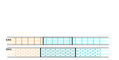
Figure 1: (Color online) Schetch of CNS [panel (a)] and GNS [panel (b)] system, in which ideal superconducting lead (left, orange), normal lead (right, blue) and disordered normal scattering region (shadowed blue region) are concluded.

The scattering theory of electronic conduction is developed by Landauer,Landauer Imry,Imry and B$\ddot{u}$ttiker.Buttiker It provides a complete description of quantum transport in the system without electron-electron interactions. A mesoscopic conductor can be modeled by a phase-coherent disordered region connected by ideal leads (without disorder) to two electron reservoirs (normal metal or superconductor), which are in equilibrium at zero temperature with fixed electrochemical potential (or Fermi energy) $E_{F}$. Here we assume that the central scattering region is normal region, the same as the right normal lead. Then the total system Hamiltonian

$$H=H_{S}+H_{N}+H_{T}$$ (1)

where $H_{S}$, $H_{N}$ and $H_{T}$ are the Hamiltonian of superconducting lead (orange region in Fig.1), semi-infinite normal ribbon (blue region in Fig.1) and tunneling between the normal region and superconducting terminal, respectively.

Two kinds of structure were considered in this paper: the structure with quadratic energy dispersion [square lattice, Fig.1(a)] and structure with conical energy spectrum [honeycomb lattice, Fig.1(b)]. In the absence of the superconductor, the whole system $H_{0}$ including $H_{S}$, $H_{N}$ and $H_{C}$ can be written in the tight-binding representation:ref19 ; ref20

$$H_{0}=\sum_{\bf i}(E_{0}+\delta\epsilon_{\bf i})a^{\dagger}_{\bf i}a_{\bf i}-\sum_{<{\bf ij}>}ta_{\bf i}^{\dagger}a_{\bf j}$$ (2)

where ${\bf i}=(i_{x},i_{y})$ is the index of the discrete square lattice or honeycomb lattice site which is arranged as in inset of Fig.1. Here $a_{\bf i}$ and $a_{\bf i}^{\dagger}$ are the annihilation and creation operators at the discrete site ${\bf i}$. $E_{0}$ is the constant on-site energy. In the square lattice, $E_{0}$ is center of energy band, and in honeycomb lattice, $E_{0}$ is the energy reference point (the Dirac Point). $\delta\epsilon_{\bf i}$ is random on-site potential which is nonzero only in the center region to simulate the disordered scattering region. Here $\delta\epsilon_{\bf i}$ is uniformly distributed with $\delta\epsilon_{\bf i}=[-w/2,w/2]$ where $w$ is disorder strength. The data for fluctuations are obtained by averaging over up to 10,000 disorder configurations and the data for distribution are obtained over 1,000,000 disorder configurations. The second term in Eq.(2) is the nearest neighbor hopping with hopping elements $t$ and “$<>$” denotes the sum over the nearest sites.

Due to the superconductor, it is convenient to write the Hamiltonian $H$ in the Nambu representation,Nambu . In this representation the Fermi energy of the right normal lead in equilibrium (at zero bias) is set to be the superconductor condensate. It is conventionally set to zero. As a result, the spin up electrons and the spin down holes have the positive and negative energy, respectively. Taking this into account the Hamiltonian (2) is cross multiplied by spin representation. $H_{N}$ and $H_{T}$ in Eq.(1) can be rewritten as $H_{0,N/T}\otimes\sigma_{z}$ and

$$H_{S}=\left(\begin{array}[]{cc}H_{0,S}&\tilde{\Delta}\\ \tilde{\Delta}^{*}&-H_{0,S}\end{array}\right)$$ (3)

where $\tilde{\Delta}=\Delta e^{i\varphi}$ is the energy gap or the pair potential of the semi-infinite superconducting lead. Here we can assume $\tilde{\Delta}=\Delta$ to be a real parameter by selecting a special phase of the superconductor lead in our calculation.realGap

In the calculation, for simplicity we set external voltage in the normal and superconducting terminal as $V_{N}=V$, $V_{S}=0$. The current flowing from the normal lead can be calculated from the Landauer-B$\ddot{u}$ttiker formula:footnote

$$J_{N}=J^{e}_{N}-J^{h}_{N}$$

$$J^{e/h}_{N}=\pm\frac{e}{\hbar}\int\frac{dE}{2\pi}~{}\left\{T_{e/h}(E)[f_{\pm}(E)-f_{0}(E)]\right.$$

$$~{}~{}~{}~{}~{}~{}~{}~{}~{}~{}~{}~{}~{}~{}~{}~{}~{}~{}~{}~{}~{}~{}\left.T_{A}(E)[f_{\pm}(E)-f_{\mp}(E)]\right\}$$ (4)

where $e$ is the electron charge, $f_{0}(E)=\left[e^{E/k_{B}\mathcal{T}}+1\right]^{-1}$ is the Fermi distribution in the superconducting lead, $f_{\pm}(E)=\left[e^{(E\mp eV_{N})/k_{B}\mathcal{T}}+1\right]^{-1}$ are the Fermi distribution functions in the normal terminal for the electrons and holes, respectively. $T_{e/h}$ is the transmission coefficient that the particles incident from superconducting lead traverse to the normal terminal as electrons/holes and $T_{A}$ is AR coefficient representing the reflection probability that the incident electrons from the normal terminal are reflected as holes or vice versa. Note that the two processes are symmetric and have the same AR coefficient $T_{A}$. $T_{e/h}$ and $T_{A}$ are calculated from

$$T_{e}={\rm Tr}\{\Gamma^{N}_{\uparrow\uparrow}[G^{r}\Gamma^{S}G^{a}]_{\uparrow\uparrow}\},~{}~{}T_{h}={\rm Tr}\{\Gamma^{N}_{\downarrow\downarrow}[G^{r}\Gamma^{S}G^{a}]_{\downarrow\downarrow}]\}$$

$$T_{A}={\rm Tr}[\Gamma^{N}_{\uparrow\uparrow}G^{r}_{\uparrow\downarrow}\Gamma^{N}_{\downarrow\downarrow}G^{a}_{\downarrow\uparrow}]={\rm Tr}[\Gamma^{N}_{\downarrow\downarrow}G^{r}_{\downarrow\uparrow}\Gamma^{N}_{\uparrow\uparrow}G^{a}_{\uparrow\downarrow}]$$ (5)

the line-width function $\Gamma^{N/S}(E)=i[\Sigma_{N/S}^{r}(E)-\Sigma_{N/S}^{r\dagger}(E)]$. The Green’s function $G^{r}(E)=[G^{a}(E)]^{\dagger}=[EI-H_{C}-\Sigma^{r}_{N}(E)-\Sigma^{r}_{S}(E)]^{-1}$ where $H_{C}$ is Hamiltonian matrix of the central scattering region and $I$ is the unit matrix with the same dimension as that of $H_{C}$, $\Sigma_{l=N,S}^{r}$ is the matrix of retarded self-energy from the normal/superconducting lead with the only nonzero elements in the sub-block that are neighbor of normal or superconducting lead. The self-energy is calculating according to $\Sigma^{r}_{l}=H_{Cl}g^{r}H_{lC}$ where $H_{Cl}$ ($H_{lC}$) is the coupling from central region (leads) to leads (central region) and $g^{r}$ is the surface retarded Green’s function of semi-infinite lead which can be calculated using a transfer matrix method.transfer Due to electron-hole symmetry, $T_{e}(E)=T_{h}(-E)$ and $T_{A}(E)=T_{A}(-E)$, which leads to $J_{N}=2J^{e}_{N}=-2J^{h}_{N}$.

At zero temperature limit, the energy dependent conductance can be expressed as:

$$G_{NS}(E_{F}) = d(J^{e}_{N}-J^{h}_{N})/dV$$ (6)

$$= \frac{e^{2}}{h}\left\{[T_{e}(E_{F})+T_{h}(-E_{F})]+4T_{A}(E_{F})\right\}$$

$$= \frac{2e^{2}}{h}\left[T_{e/h}(\pm E_{F})+2T_{A}(E_{F})\right].$$

When the incident energy $E_{F}<\Delta$, there is no normal quasi-particle transport $T_{e/h}=0$ and only AR contributes to conductance $G$. We will focus mainly on this quantity in this paper. In this case, the conductance fluctuation defined as ${\rm rms}(G)=\sqrt{\langle[G-\langle G\rangle]^{2}\rangle}$ becomes

$${\rm rms}(G)=\frac{4e^{2}}{h}\sqrt{\langle T_{A}^{2}\rangle-\langle T_{A}\rangle^{2}}$$ (7)

where $\langle...\rangle$ denotes averaging over an ensemble of samples with different disorder configurations of the same strength $w$. When $E_{F}$ is beyond superconducting energy gap $\Delta$, normal transmission $T_{e/h}$ is present, conductance variance now consists of three components: (1). the Andreev related fluctuation ${\rm Var}(G)_{\rm Andr}$ from AR coefficient $T_{A}$. (2). the normal fluctuation ${\rm Var}(G)_{\rm Norm}$ from normal transmission coefficient $T_{e/h}$. (3). the cross term ${\rm Var}(G)_{\rm cross}$. They are expressed as

$${\rm Var}(G)={\rm Var}(G)_{\rm Andr}+{\rm Var}(G)_{\rm Norm}+{\rm Var}(G)_{\rm cross}$$

$$=[\frac{e^{2}}{h}]^{2}\left[\left\langle(4\delta T_{A})^{2}\right\rangle+\left\langle(\delta T_{N})^{2}\right\rangle+8\left\langle\delta T_{A}\delta T_{N}\right\rangle\right]$$ (8)

where $\delta T_{A}=T_{A}-\langle T_{A}\rangle$, $\delta T_{N}=(T_{e}+T_{h})-\langle T_{e}+T_{h}\rangle$.

III results and discussion

In the numerical calculations, the energy is measured in the unit of the nearest coupling elements $t$. For the square lattice, $t=\frac{\hbar^{2}}{2m^{*}a^{2}}$ with $m^{*}$ the effective electron mass and $a$ the lattice constant. For the honeycomb lattice, $t=\frac{2}{3b}\hbar v_{F}$ with the carbon-carbon distance $b=0.142nm$ and the Fermi velocity $v_{F}=0.89\times 10^{6}ms^{-1}$. The size of the scattering region $N\times M$ is described by integer $N$ and $M$ corresponding to the width and length, respectively. For example in Fig.1, the width $W=Na$ with $N=3$, the length $L=Ma$ with $M=5$ in the panel (a), and the width $W=N\times 3b$ with $N=3$, the length $L=M\times\sqrt{3}b$ with $M=7$ in the panel (b).

Table 1: The parameter $E_{F}$, $E_{0}$, $\Delta$ used in the square lattice model and honeycomb model. The different columns are corresponding to the different transport processes denoted by ‘AR’, ‘ARR’, ‘SAR’ ,‘NT’ and so on. Here, ‘AR’ is for the pure conventional AR assisted tunneling processes (only conventional AR exists) in square lattice. ‘ARR‘ and ‘SAR’ denotes the pure ARR assisted process and pure SAR assisted process in honeycomb lattice, respectively. ‘NT’ is for the transport beyond the superconducting Gap where NT can also contribute to the transport processes.

sq
AR	$E_{F}$	$E_{0}$	$\Delta$	AR	$E_{F}$	$E_{0}$	$\Delta$	NT	$E_{F}$	$E_{0}$	$\Delta$
1	0	2.1	0.1	4	0.2	2.2	0.3	1	0.2	2.2	0.3
2	0	2.3	0.1	5	0.3	2.3	0.4	2	0.3	2.3	0.4
3	0	2.4	0.1	6	0.4	2.4	0.5	3	0.4	2.4	0.5
hc
ARR	$E_{F}$	$E_{0}$	$\Delta$	SAR	$E_{F}$	$E_{0}$	$\Delta$	NT	$E_{F}$	$E_{0}$	$\Delta$
1	0	0.6	0.1	1	0.6	0.0	0.7	1	0.7	0	0.5
2	0	0.7	0.1	2	0.6	0.1	0.7	2	0.7	0.1	0.5
3	0	0.8	0.1	3	0.7	0.0	0.8	3	0.7	0	0.3
4	0	0.9	0.1	4	0.7	0.1	0.8	4	0.7	0.1	0.3
5	0.1	0.7	0.2					5	0.7	0	0.1
6	0.1	0.8	0.2					6	0.7	0.1	0.1

As documented in the literature, in order to get the saturated UCF plateaus,saenz2 ; ucf4 ; LiDafang the number of transmission channels for incoming electron should be large enough in the numerical calculation. We denote $N_{c}$ as the chain number which determines directly the number of channels. $N_{c}$ is defined in the following way: take Fig.1 as an example, in panel (a), $N_{c}=3$ and $N_{c}=6$ in panel (b). In 2D systems we set $N_{c}=40$ and $60$. For quasi 1D systems we use only $N_{c}=40$ because it is more computational demanding than 2D systems. To get a larger channel number, the incident energy $E_{F}$ should be set away from the bottom of energy band $E_{b}$. In the square lattice, to mimic the parabolic energy spectrum for Fermi electrons, the constraints for incident energy $E_{F}<E_{b}+2t$ and Andreev reflected energy $-E_{F}<E_{b}+2t$ are needed. While for Dirac electrons in the honeycomb lattice, the absolute value of relative incident energy (to the Dirac point $E_{0}$) $|E_{F}-E_{0}|<t$ and relative Andreev reflected energy $|-E_{F}-E_{0}|<t$ are set.

In Table.1, we list all the parameters used in the following calculations including the incident energy $E_{F}$, the superconducting gap $\Delta$ and the on-site energy $E_{0}$ which is the center of energy band for the square lattice and the Dirac Point for the honeycomb lattice. From these parameters in the clean system with NS heterojunction, we can easily calculate the channel number for electron or hole, AR coefficient $T_{A}$ and the normal transmission coefficient of electron or hole $T_{se/sh}$ for Fermi energy beyond superconducting gap. At the same time, we can also get the normal transmission coefficient $T_{ne/nh}$ in normal system without the superconducting lead.

III.1 Conductance fluctuation and conductance distribution in the diffusive regime

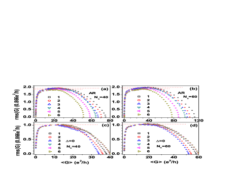
Figure 2: (Color online) panel(a) and panel(b): in the presence of superconducting lead, conductance fluctuation ${\rm rms}(G)$ vs average conductance $\langle G\rangle$ in the square lattice for $N_{c}=40$ and $N_{c}=60$, respectively. The symbol is labeled in first column in Tab.1 for the square lattice case denoted by ‘sq’. The red dotted lines indicate two plateaus in the values (with the unit of $0.866e^{2}/h$) of $1.94\pm 0.03$ and $1.85\pm 0.05$ in panel (a) and $1.98\pm 0.02$ and $1.89\pm 0.03$ in panel (b). For comparison, corresponding to panel (a) and panel (b), in panel (c) and (d), we plot ${\rm rms}(G)$ vs $\langle G\rangle$ in the absence of superconducting lead, i.e., $\Delta=0$, respectively. The plateaus in the values of $1.02\pm 0.02$ and $1.04\pm 0.02$ in the unit of $0.866e^{2}/h$ are indicated in panel (c) and panel (d). The system size: $N_{c}=40$ corresponds to width $W=40a$, considering the square shape sample, we set $L=40a$. For $N_{c}=60$, we have $W=60a$, $L=60a$.

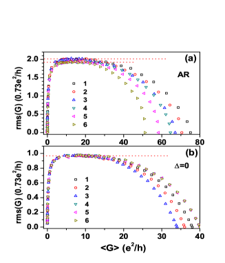
Figure 3: (Color online) Same as Fig.2 except the model is quasi-1D square lattice with chain number $N_{c}=40$. The system size: width $W=40a$, length $L=1000a$. In the unit of $0.73e^{2}/h$, two plateaus with the values of $2.01\pm 0.02$ and $1.93\pm 0.03$ in panel (a) and a single plateau in the value of $0.97\pm 0.01$ is indicated in panel (b).

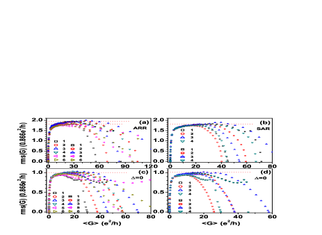
Figure 4: (Color online) ${\rm rms}(G)$ contributed by ARR [panel(a)] and SAR [panel(b)] vs $\langle G\rangle$ in 2D honeycomb lattice for $N_{c}=40$ [open symbols] and $N_{c}=60$ [symbols with ‘-’]. The symbols are labeled in second column in Tab.1 for the honeycomb lattice case denoted by ‘hc’. The red dotted lines indicate two plateaus with the values of $1.96\pm 0.03$ and $1.82\pm 0.02$ in the unit of $0.866e^{2}/h$ in panel (a) and a single plateau with the value of $1.82\pm 0.02$ in panel (b). Panel (c) and (d): ${\rm rms}(G)$ contributed by normal quasi-particle transmission $T_{ne}$ vs $\langle G\rangle$ in case of $\Delta=0$, corresponding to panel (a) and (b), respectively. The plateaus in the values of $1.00\pm 0.02$ in the unit of $0.866e^{2}/h$ are indicated in panel (c) and panel (d). The system size: for $N_{c}=40$ its width is equal to $W=60b$; considering the square shape sample, the length $L=35\sqrt{3}b$. Similarly, for $N_{c}=40$ its width is $W=90b$, $L=52\sqrt{3}b$.

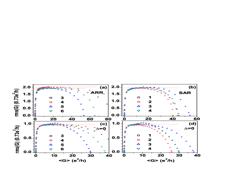
Figure 5: (Color online) Same as Fig.2 except the model is quasi-1D honeycomb lattice with chain number $N_{c}=40$. The system size: width $W=60b$, length $L=500\sqrt{3}b$. The red dotted lines indicate two plateaus with the values of $2.03\pm 0.03$ and $1.93\pm 0.03$ in the unit of $0.73e^{2}/h$ in panel (a), a single plateau with the value of $1.94\pm 0.04$ in panel (b), the value of $0.98\pm 0.02$ in panel (c) and panel (d).

We first examine conductance fluctuations in the diffusive regime. In our calculation the size of 2D square lattice is set to be $40\times 40$ for $N_{c}=40$ and $60\times 60$ for $N_{c}=60$. The size of 2D honeycomb lattice is chosen to be $20\times 35$ for $N_{c}=40$ and $30\times 52$ for $N_{c}=60$. For quasi-1D systems, the size is chosen to be $40\times 1000$ in square lattice and $20\times 500$ in honeycomb lattice with $N_{c}=40$. In Fig.2 and 3, 4 and 5, we plot conductance fluctuations ${\rm rms}(G)$ vs the average conductance $\langle G\rangle$ in 2D square lattice, quasi-1D square lattice, 2D honeycomb lattice and quasi-1D honeycomb lattice, respectively. Each point in the figure is obtained by averaging over 10,000 configurations. Different parameters used in all figures are tabulated in Table.1.

From Fig.2-5, we see following general behaviors. (1). in the localized regime where $\langle G\rangle<1$, all the curves collapse into a single curve indicating the universal behavior of the conductance distribution function.ucf4 (2). in the diffusive regime where $\langle G\rangle>1$, there is a plateau region for ${\rm rms}(G)$ where the fluctuation is nearly independent of average conductance $\langle G\rangle$ and other system parameters. This is the regime for the universal conductance fluctuation. The plateau value [labeled by red dotted line in top panels] is approximately twice the value of the known UCF values ${\rm rms}(G)=0.866e^{2}/h$ for 2D system and $0.73e^{2}/h$ for quasi-1D system [labeled by red dotted line in bottom panels]. This doubling seems to be true for both Fermi electrons (square lattice) [Fig.2 and Fig.3] and Dirac electrons (graphene system) [Fig.4 and Fig.5]. (3). There are two separate UCF plateaus for the AR assisted transport processes in the CNS system [Fig.2(a), Fig.3(a)] and the ARR assisted transport processes in GNS system [Fig.4(a),Fig.5(a)], while for the SAR assisted transport processes [panel (b)] there is only one UCF plateau. It appears that this difference in UCF can be used to distinguish ARR and SAR. However, it turns out to be incorrect when considering the ehD “symmetry”. In Fig.4(a) and Fig.5(a), Andreev conductance fluctuations corresponding to $E_{F}=0$ (with ehD) and $E_{F}\neq 0$ (ehD broken) from diffusive regime all the way to localized regime are plotted and two UCF plateaus associated to ehD “symmetry” are then indicated. For SAR in graphene systems, we have $|E_{F}|>|E_{0}|\neq 0$ (ehD broken). Fig.4(b) and Fig.5(b) then show only one UCF plateau. (4). Denoting the increase factor $\alpha_{0}$ through the relation ${\rm rms}(G_{NS})=\alpha_{0}~{}{\rm rms}(G_{N})$ [$G_{N}$ is shown in bottom panels in Fig.2-5] in the plateau region in diffusive regime, it is very different for square 2D system and quasi-1D system and slightly different for Fermion electrons and Dirac electrons. Specifically, our results for the quasi-1D systems for both Fermi electrons and Dirac electron is as follows: (a). when ehD is present ${\rm rms}(G_{NS})/{\rm rms}(G_{N})$ is $2.07\pm 0.04$ that is very close to $\sqrt{4.3}$. (b). when ehD is broken it is $1.99\pm 0.08$ that is close to $\sqrt{4}$. For 2D systems, when ehD is present, ${\rm rms}(G_{NS})/{\rm rms}(G_{N})$ is $1.91\pm 0.07$ for Fermi electrons and $1.96\pm 0.07$ for Dirac electrons. When ehD is broken it is $1.82\pm 0.08$ for both Fermi electrons and Dirac electrons. (5). For larger $\langle G\rangle$ (in the ballistic regime) the conductance fluctuation falls down quickly to zero. This is because the number of conducting channels $N_{c}$ is finitesaenz2 ; LiDafang ; ucf4 . The width of plateau region is longer with a larger $N_{c}$. In the limit of the infinite $N_{c}$, the plateaus of conductance fluctuation will extend to infinite.

We now take a closer look at each figure discussed above. In the top panels of Fig.2-5, we can see that all curves of ${\rm rms}(G)$ vs $\langle G\rangle$ collapse into universal curves that are slightly separated in the region of $1<\langle G\rangle<10$. To make the discussion of separate UCF plateaus quantitative, we plot ${\rm rms}(G)$ vs small $\langle G\rangle$ ($\langle G\rangle<10$) in Fig.6(a), (b), (c) and (d) corresponding to Fig.2, Fig.3, Fig.4 and Fig.5. In Fig.6, we clearly see two separate UCF in the regime where $1<\langle G\rangle<10$. For each UCF plateau, the conductance fluctuation ${\rm rms}(G)$ vs average conductance $\langle G\rangle$ is a universal function, i.e., it is independent of system parameters such as $E_{F}$, $E_{0}$, $\Delta$, system size and so on and depends only on $\langle G\rangle$. In fact, not only the ${\rm rms}(G)$ (the second moment), the third, forth, …, and higher moments are universal function of $\langle G\rangle$. This means that the conductance distribution $P(G)$ is a universal function that depends only on the average conductance $\langle G\rangle$ in addition to the symmetry and dimensionality of the system.

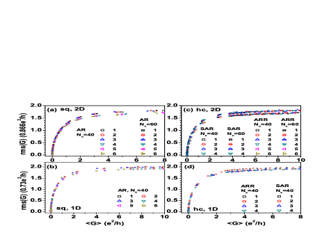
Figure 6: (Color online) Corresponding to Fig.2, Fig.3, Fig.4 and Fig.5, ${\rm rms}(G)$ vs small $\langle G\rangle$ ($<10$) are plotted in panel(a), (b), (c) and (d), respectively.

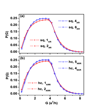
Figure 7: (Color online) In the diffusive regime, corresponding to eight selected parameters with $|E_{F}|<\Delta$ from Tab.1, the conductance distribution $P(G)$ obtained from 1,000,000 configurations is plotted for the fixed $\langle G\rangle\simeq 3$ in square [panel (a)] and honeycomb lattices [panel (b)].

Table 2: In square lattice or honeycomb model, corresponding to eight selected parameter labeled in Tab.1 with $|E_{F}|>\Delta$, the average conductance $\langle G\rangle$ and the second, third, …, ninth moments are listed for the first (with ehD, 1 and 3 column) and the second (ehD broken, 2 and 4 column) class in the diffusive regime with $\langle G\rangle\simeq 3$.

sq	$\langle G\rangle$	$\sqrt{\mu_{2}}$	$\sqrt[3]{\mu_{3}}$	$\sqrt[4]{\mu_{4}}$	$\sqrt[5]{\mu_{5}}$	$\sqrt[6]{\mu_{6}}$	$\sqrt[7]{\mu_{7}}$	$\sqrt[8]{\mu_{8}}$	$\sqrt[9]{\mu_{9}}$
$1_{\rm AR}$	3.001	1.445	0.929	1.840	1.750	2.196	2.266	2.512	2.645
$2_{\rm AR}$	3.013	1.443	0.923	1.838	1.745	2.184	2.266	2.518	2.660
$4_{\rm AR}$	2.986	1.366	0.862	1.737	1.639	2.061	2.129	2.367	2.486
$6_{\rm AR}$	2.976	1.365	0.864	1.736	1.639	2.061	2.129	2.367	2.486
hc	$\langle G\rangle$	$\sqrt{\mu_{2}}$	$\sqrt[3]{\mu_{3}}$	$\sqrt[4]{\mu_{4}}$	$\sqrt[5]{\mu_{5}}$	$\sqrt[6]{\mu_{6}}$	$\sqrt[7]{\mu_{7}}$	$\sqrt[8]{\mu_{8}}$	$\sqrt[9]{\mu_{9}}$
$1_{\rm ARR}$	2.998	1.417	0.899	1.805	1.708	2.143	2.218	2.463	2.591
$2_{\rm ARR}$	2.988	1.421	0.901	1.809	1.713	2.148	2.224	2.470	2.602
$5_{\rm ARR}$	3.005	1.347	0.836	1.713	1.606	2.031	2.091	2.328	2.441
$4_{\rm SAR}$	3.009	1.344	0.833	1.710	1.602	2.027	2.087	2.324	2.438

To demonstrate the conductance distribution has two different universalities, we plot in Fig.7 the conductance distribution $P(G)$ obtained from 1,000,000 configurations for a fixed average conductance $\langle G\rangle\simeq 3$ in the square lattice [panel (a)] and the honeycomb lattice [panel (b)]. In this figure, we choose eight parameters from Tab.1 with $|E_{F}|<\Delta$. We see that for both square and honeycomb lattices, the conductance distributions corresponding to $E_{F}=0$ and $E_{F}\neq 0$ are clearly different. In addition, for each case, $E_{F}=0$ or $E_{F}\neq 0$, conductance distributions for square and honeycomb lattices are almost the same, as can be seen from Tab.2 in which the second, third, …, ninth moments are listed for the parameters labeled in Tab.1 corresponding to the first ($E_{F}=0$ with ehD) and the second ($E_{F}\neq 0$ where ehD is broken) classes with fixed $\langle G\rangle\simeq 3$. Here, the n-th moment is defined as $\mu_{n}=\left\langle[G-\langle G\rangle]^{n}\right\rangle$. In Tab.2, the n-th moments labeled by “$1_{AR}$” and “$2_{AR}$” correspond to the first class in square lattice, they are close to the n-th moments labeled by ‘$1_{ARR}$’ and ‘$2_{ARR}$’ in honeycomb lattice. Since the universal behavior is determined only by the symmetry and dimensionality, why there are two universal curves for AR? This can be qualitatively understood as follows.

When the energy of incoming electron is within the superconducting energy gap, only AR exists. The AR amplitude of total NS system $T_{A}$ is contributed by multiple Andreev reflections and can be expressed in terms of transmission amplitude $t$ and $r$ in the absence of superconducting leads and the pure AR matrix $r_{A}$ of the only NS interface [not consider the clean or disordered normal scattering region] in the following formBeenakker

$$T_{A}(\epsilon)={\rm Tr}[m(\epsilon)m^{\dagger}(\epsilon)]$$ (9)

with

$$m(\epsilon)=t^{e}_{12}(\epsilon)Mt^{e,\dagger}_{12}(-\epsilon)$$

$$M=[I-r^{eh}_{A}(\epsilon)r^{e,*}_{22}(-\epsilon)r^{eh,T}_{A}(\epsilon)r^{e}_{22}(\epsilon)]^{-1}r^{eh}_{A}(\epsilon)$$ (10)

where we have used the electron-hole symmetry relation $t^{h}_{21}(\epsilon)=t^{e,*}_{21}(-\epsilon)$, $r^{he}_{A}(\epsilon)=r^{eh,T}_{A}(\epsilon)$ and the symmetry relation of normal transmission matrix $t^{e}_{21}(\epsilon)=t^{e,T}_{12}(\epsilon)$ in the absence of magnetic filed, where ‘T’ denotes transpose. Eq.(10) can be expanded in power series which gives multiple Andreev reflections. For qualitative understanding, we can focus on the first term in the series, i.e., $m(\epsilon)=t_{12}(\epsilon)t_{12}^{\dagger}(-\epsilon)$ and $T^{(1)}_{A}=T_{12}(\epsilon)T_{12}(-\epsilon)$. It is similar for the higher order of $T_{A}$. Now it is clear why we obtain two universal conductance distributions for Andreev conductance. For $\epsilon=0$ (with ehD) the total Andreev reflection coefficient $T_{A}$ is expressed in terms of only one type of normal transmission coefficient $T(0)$. For $\epsilon\neq 0$ (ehD broken), however, $T_{A}$ consists of two kinds of transmission coefficient $T(\epsilon)$ and $T(-\epsilon)$ that have the completely different statistics. It is the statistical interference of $T(\epsilon)$ and $T(-\epsilon)$ that leads to the new universal conductance distribution.

It should be noted in order to get the uniform statistical interference, $T(\epsilon)$ and $T(-\epsilon)$ must be separated far enough from each other, i.e., $\epsilon$ is larger than Thouless energy. The incident energy $\epsilon$ (related to condensed energy, equal to $E_{F}$ in our calculation) is so large that it is comparable to energy gap $\Delta$, so we must go beyond Andreev approximation (AA). While in the present works, AA are widely used, it is why the present works can’t present this new symmetry class. We will show [Fig.9] in the AA, the conductance distribution is smoothly changed with $E_{F}$, in stead of the two universal functions corresponding to $E_{F}=0$ and $E_{F}\neq 0$ in the case with non-Andreev approximation (NAA).

III.2 Statistical properties in the localized regime

As we have shown, different universal conductance distributions corresponding to $E_{F}=0$ and $E_{F}\neq 0$ are found in the diffusive regime. It has been demonstrated numericallyucf4 that the conductance distribution for a fixed $\langle G\rangle$ in the localized regime seems to be a universal function which does not depend on dimensionality (quasi-1D, 2D and quantum dot systems) and ensemble symmetry (COE, CUE or CSE). For normal-superconductor hybrid systems, it is interesting to know whether this conclusion is still valid.

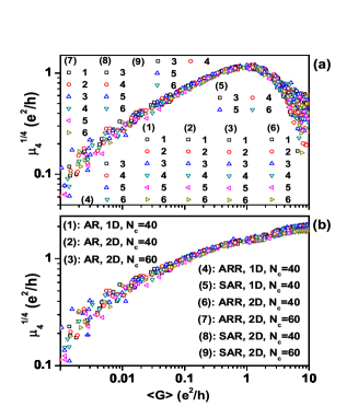
Figure 8: (Color online) the skewness $\gamma_{1}$ and the kurtosis $\gamma_{2}$ vs $\langle G\rangle$ for the 1D square or honeycomb lattice with $N_{c}=40$ and 2D square or honeycomb lattice with $N_{c}=40$ and $N_{c}=60$. Different symbols (1)-(9) are described as in panel (b) and labeled in Tab.1.

Table 3: Same to Tab.2 except we consider localized regime with fixed average conductance $\langle G\rangle\simeq 0.3$.

sq	$\langle G\rangle$	$\sqrt{\mu_{2}}$	$\sqrt[3]{\mu_{3}}$	$\sqrt[4]{\mu_{4}}$	$\sqrt[5]{\mu_{5}}$	$\sqrt[6]{\mu_{6}}$	$\sqrt[7]{\mu_{7}}$	$\sqrt[8]{\mu_{8}}$	$\sqrt[9]{\mu_{9}}$
$1_{\rm AR}$	.3005	0.669	0.986	1.287	1.527	1.728	1.900	2.052	2.192
$2_{\rm AR}$	.2997	0.669	0.986	1.287	1.527	1.727	1.898	2.049	2.186
$4_{\rm AR}$	.3002	0.632	0.936	1.229	1.464	1.658	1.823	1.964	2.087
$6_{\rm AR}$	.2990	0.631	0.936	1.229	1.464	1.660	1.826	1.970	2.099
hc	$\langle G\rangle$	$\sqrt{\mu_{2}}$	$\sqrt[3]{\mu_{3}}$	$\sqrt[4]{\mu_{4}}$	$\sqrt[5]{\mu_{5}}$	$\sqrt[6]{\mu_{6}}$	$\sqrt[7]{\mu_{7}}$	$\sqrt[8]{\mu_{8}}$	$\sqrt[9]{\mu_{9}}$
$1_{\rm ARR}$	.2998	0.667	0.982	1.281	1.520	1.718	1.887	2.036	2.170
$2_{\rm ARR}$	.3005	0.669	0.985	1.286	1.526	1.725	1.895	2.044	2.179
$5_{\rm ARR}$	.3001	0.631	0.934	1.226	1.460	1.654	1.817	1.958	2.081
$4_{\rm SAR}$	.3002	0.631	0.936	1.229	1.463	1.658	1.823	1.966	2.094

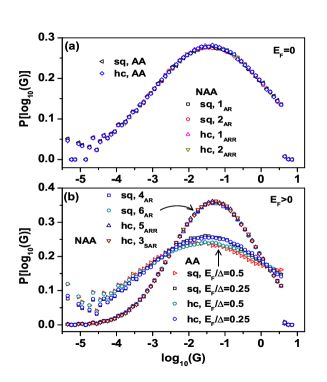
Figure 9: (Color online) In the localized regime, corresponding to selected parameters labeled in Tab.1 with $|E_{F}|=0$ and $0<|E_{F}|<\Delta$, the conductance distribution $P[\log_{10}(G)]$ obtained from 1,000,000 configurations are plotted in panel (a) and panel(b) respectively for the fixed $\langle G\rangle\simeq 0.3$ in square lattice [marked with sq] and honeycomb lattice [marked with hc]. In addition, we also plot $P[\log_{10}(G)]$ within AA for $E_{F}=0$ and $E_{F}\neq 0$ in panel(a) and panel(b), respectively.

There are two ways to examine the universal conductance distribution $P(G)$: (1). plot $P(G)$ at each $\langle G\rangle$ for different system parameters to see whether all $P(G)$ collapse into a single curve. One can only plot $P(G)$ at a few selected $\langle G\rangle$. (2). plot the moments of $P(G)$ as a function of $\langle G\rangle$ to see the universal behavior. However one can only plot several moments of conductance. Here we focus on the higher order moments $\mu_{3}$ and $\mu_{4}$. In Fig.8, we plot $\sqrt[3]{\mu_{3}}$ [panel(a)] and $\sqrt[4]{\mu_{4}}$ [panel(4)] vs $\langle G\rangle$ for 2D and quasi-1D systems on square and honeycomb lattices. Symbols (1)-(9) are described as in panel (b) and labeled in Tab.1. From the figure, it is clear that the data do not collapse into a single curve. In this calculation, we have used only 10,000 configurations per data point which is not enough to resolve the universality class if any. To improve this, we fix the average conductance $\langle G\rangle$ and calculate higher moments by averaging over 1,000,000 configurations. In Tab.3, we choose the same set of parameters as used in the diffusive regime [Tab.2], and tabulate the average conductance $\langle G\rangle$ and the second, third, …, ninth moments for the fixed $\langle G\rangle\simeq 0.3$. Similar to Tab.2, two universality classes can be identified. The first universality class has ehD and consists of data points from four different set of parameters labeled by “$1_{AR}$” and “$2_{AR}$”(square lattice) and labeled by “$1_{ARR}$” and “$2_{ARR}$”(honeycomb lattice). The rest of data form the second universality class where ehD is broken. Hence it is expected that the conductance distributions for $E_{F}=0$ (with ehD) and $E_{F}\neq 0$ (without ehD) belong to different universality class in the localized regime. This indeed can be seen from Fig.9(a) and (b) where we have plotted the conductance distributions of $\log_{10}(G)$ for $E_{F}=0$ and $E_{F}\neq 0$. Fig.9(a) shows the conductance distribution with ehD for six different sets of parameters where two of them are for AA and the other four are NAA. Obviously, they fall into the same universality class. In Fig.9(b), we show the data for the case with broken ehD. We see that four set of data with NAA collapse into a single curve indicating the universal conductance distribution that is clearly different from Fig.9(a). When AA is made, however, the conductance distribution depends on $E_{F}$ which is non-universal. The results from Fig.9 show that even in the localized regime, the Andreev conductance distributions for $E_{F}=0$ (with ehD) and $E_{F}\neq 0$ (ehD broken) belong to different universality class.

III.3 statistics beyond superconducting gap

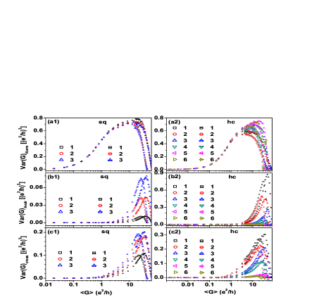
Figure 10: (Color online) ${\rm Var}(G)_{\rm Norm}$, ${\rm Var}(G)_{\rm Andr}$ and ${\rm Var}(G)_{\rm cross}$, the three compositions of variance of $G$ vs $\langle G\rangle$ for the 2D square lattice [the left column] and 2D honeycomb lattice [the right column] with $N_{c}=40$ [open symbols] and $N_{c}=60$ [symbols with ‘-’].

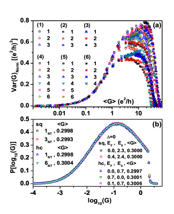
Figure 11: (Color online) Panel (a): ${\rm Var}(G)_{\rm Norm}$ vs $\langle G\rangle$ for the 1D [with $N_{c}=40$, corresponding to the crossed symbols] or 2D [with $N_{c}=40$, corresponding to the open symbols and $N_{c}=60$, corresponding to the symbols with ‘-’] square lattice [symbols (1), (2) and (3)] or honeycomb lattice [symbols (4), (5) and (6)]. Panel (b): in a 2D square or honeycomb lattice system with $N_{c}=40$, corresponding to four selected parameter with $E_{F}$ beyond $\Delta$ and labeled in Tab.1, conductance distribution $P[\log_{10}(G)]$ exported from 1,000,000 configurations is plotted. In comparation, we also plot $P[\log_{10}(G)]$ for different parameters in the normal system with $\Delta=0$ from 1,000,000 configurations.

Table 4: Beyond the superconducting Gap $\Delta$, the average conductance $\langle G\rangle$ and the second, third, …, ninth moments of normal conductance $G_{N}$ are listed in the localized regime with $\langle G\rangle\simeq 0.3$.

NT	$\langle G\rangle$	$\sqrt{\mu_{2}}$	$\sqrt[3]{\mu_{3}}$	$\sqrt[4]{\mu_{4}}$	$\sqrt[5]{\mu_{5}}$	$\sqrt[6]{\mu_{6}}$	$\sqrt[7]{\mu_{7}}$	$\sqrt[8]{\mu_{8}}$	$\sqrt[9]{\mu_{9}}$
$1_{\rm sq}$	.2997	0.311	0.356	0.470	0.546	0.622	0.691	0.755	0.814
$3_{\rm sq}$	.2999	0.310	0.355	0.467	0.544	0.620	0.689	0.752	0.812
$1_{\rm hc}$	.2998	0.310	0.357	0.472	0.551	0.631	0.703	0.771	0.835
$6_{\rm hc}$	.3004	0.310	0.351	0.462	0.537	0.612	0.679	0.742	0.801

In previous sub-sections, we have studied the statistical properties of pure AR assisted conductance with incident energy $|E_{F}|<\Delta$. In this sub-section, we will focus on the case in which the incident energy $E_{F}$ is above $\Delta$. In this case, conductance is contributed by both normal transmission and Andreev reflection. The conductance variance ${\rm Var}(G)$ consists of three terms, the Andreev conductance fluctuation ${\rm Var}(G)_{\rm Andr}$, the normal conductance fluctuation ${\rm Var}(G)_{\rm Norm}$ and the cross term between them ${\rm Var}(G)_{\rm cross}$ [see Eq.(6) and Eq.(8)]. In Fig.10, we plot ${\rm Var}(G)_{\rm Norm}$, ${\rm Var}(G)_{\rm Andr}$ and ${\rm Var}(G)_{\rm cross}$ vs $\langle G\rangle$ for the 2D square lattice [left panels] and 2D honeycomb lattice [right panels] with $N_{c}=40$ [open symbols] and $N_{c}=60$ [symbols with ‘-’]. Our results can be summarized as follows. (1) The Andreev related variance ${\rm Var}(G)_{\rm Andr}$ is drastically suppressed by the disorder. In localized regime [$\langle G\rangle<1$], due to strong disorder, it is completely suppressed to almost zero. As a result only ${\rm Var}(G)_{\rm Norm}$ plays a dominant pole in the localized regime. (2) in the localized regime, the dominant ${\rm Var}(G)_{\rm Norm}$ exhibits a universal behavior, i.e., it is independent of system parameters (such as $E_{F}$, $E_{0}$, $N_{c}$, $\Delta$ and so on). In Fig.11(a), we plot ${\rm Var}(G)_{\rm Norm}$ of 2D system [Fig.10(b1),(b2)] and quasi-1D system for square lattice and honeycomb lattice. We find that ${\rm Var}(G)_{\rm Norm}$ in the localized regime is also independent of dimensionality and type of lattice. It is not surprising since in localized regime, all AR related process are suppressed by the strong disorder. In absence of electron-hole conversion, statistics of NS system are same as that of normal system.

In order to improve the accuracy in the calculation, we also calculate the higher order moments and conductance distribution by averaging over 1,000,000 configurations and tabulate average conductance $\langle G\rangle$ and the second, third, …, ninth moments for the fixed $\langle G\rangle\simeq 0.3$ in Tab.4. It is found that the n-th moment for the square lattice and the honeycomb lattice are the same. Correspondingly, in Fig.11(b), we plot the conductance distribution of $\log_{10}(G)$ in a 2D square and honeycomb lattices with $\Delta=0$ and $\Delta\neq 0$. The symbols for $\Delta\neq 0$ are labeled as in Tab.1 and the symbols for $\Delta=0$ is described in Fig.11(b). We see that those data labeled by “$1_{NT}$” belong to the first class ($E_{F}=0$), and the other data belong to the second class ($E_{F}\neq 0$). We can see that when the incident energy is above the superconducting gap $\Delta$, the conductance distributions of NS system are almost indistinguishable from that of normal system with $\Delta=0$. This again confirms that the normal transmission is dominant, electron-hole conversion and consequently the ehD is irrelevant in the localized regime.

On experimental side, conductance fluctuationstaley ; aris and magnetoconductance fluctuationbra has been measured for mono and multi-layer graphene normal systems. The conductance fluctuations of normal-superconducting hybrid systems (non-graphene) has also been studied.hartog Hence, our results can be checked experimentally.

IV conclusion

Using the tight-binding model, we have carried out a theoretical study on the sample to sample fluctuation in transport properties of phase coherent systems with conventional NS hybrid systems or graphene based NS hybrid systems. Extensive numerical simulations on quasi-1D or 2D systems show that (1). When $E_{F}<\Delta$, the UCF due to AR is found to be roughly doubled comparing to the system in the absence of the superconducting lead. Denoting the increase factor $\alpha_{0}$ through the relation ${\rm rms}(G_{NS})=\alpha_{0}~{}{\rm rms}(G_{N})$, we found that the difference between $\alpha_{0}$ in 2D system and quasi-1D system is quite large while the difference is small between Fermi electrons and Dirac electrons. (2). Our results show that ehD in the NS hybrid system can lead to a new universality class. In the diffusive regime we found two slightly separated UCF plateaus, one corresponds to the complete electron-hole symmetry class (with ehD) and the other to conventional electron-hole conversion (with ehD broken). In addition, the AR conductance distribution for the fixed average conductance $\langle G\rangle$ in diffusive regime also confirms that the new universality class can be classified using ehD. (3). In the localized regime, we found that the conductance distribution is a universal function that depends only on the average conductance and the ehD. We emphasize that one has to go beyond AA to make sure that the AR conductance distribution is universal in the localized regime. (4). Finally, when $E_{F}$ is beyond $\Delta$, normal transport is present. In general, the conductance distributions of NS systems and normal systems are different. In the localized regime, however, the AR is suppressed significantly by the disorder. Hence in the localized regime normal transmission dominates the transport processes. In this case, the ehD is irrelevant and the conductance distribution is a universal function that depends only on the average conductance in the localized regime.

$${\bf ACKNOWLEDGMENTS}$$

We gratefully acknowledge the financial support by a RGC grant (HKU705409P) from the Government of HKSAR.

References

- (1) lectronic address: jianwang@hkusua.hku.hk
- (2) B. L. Altshuler, P. A. Lee, and R. A. Webb, Mesoscopic Phenomena in Solids (North-Holland, Amsterdam, 1991).
- (3) C. W. J. Beenakker, Rev. Mod. Phys. 69, 731 (1997).
- (4) N.J. Zhu, H. Guo, and R. Harris, Phys. Rev. Lett. 77, 1825 (1996); H. U. Baranger and P. A. Mello, Phys. Rev. Lett. 73, 142 (1994); D. V. Savin, H.-J. Sommers, and W. Wieczorek, Phys. Rev. B 77, 125332 (2008); S. Hemmady, J. Hart, X. Zheng, T. M. Antonsen, Jr., E. Ott, and S. M. Anlage, Phys. Rev. B 74, 195326 (2006); Ph. Jacquod and R. S. Whitney, Phys. Rev. B 73, 195115 (2006).
- (5) P. A. Lee and A. D. Stone, Phys. Rev. Lett. 55, 1622 (1985); L. B. Altshuler, JETP Lett. 41, 648 (1985).
- (6) A. Garcia-Martin and J.J. Saenz, Phys. Rev. Lett. 87, 116603 (2001); L. S. Froufe-Pérez, P. Garcĺa-Mochales, P. A. Serena, P. A. Mello, and J. J. Sáenz, Phys. Rev. Lett. 89, 246403 (2002).
- (7) Z. Qiao, Y. Xing and J. Wang, Phys. Rev. B, 81, 085114 (2010).
- (8) C. W. J. Beenakker, Phys. Rev. B, 47, 15763 (1993).
- (9) P. W. Brouwer and C. W. J. Beenakker, Phys. Rev. B, 52, R3868 (1995).
- (10) Y. Takane and H. Ebisawa, J. Phys. Soc. Jpn. 61, 2858 (1992); J. Bruun, V. C. Hui and C. J. Lambert, Phys. Rev. B, 49, 4010 (1994).
- (11) A. Altland and Martin R. Zirnbauer, Phys. Rev. B, 55, 1142 (1997).
- (12) Y. Takane and H. Ebisawa, J. Phys. Soc. Jpn. 60, 3130 (1991)
- (13) H.B. Heersche, P. Jarillo-Herrero, J.B. Oostinga, L.M.K. Vandersypen, and A.F. Morpurgo, Nature 446, 56 (2007).
- (14) F. Miao, S. Wijeratne, Y. Zhang, U.C. Coskun, W. Bao, and C.N. Lau, Science 317, 1530 (2007).
- (15) A.F. Andreev, Sov. Phys. JETP 19, 1228 (1964).
- (16) C.W.J. Beenakker, Phys. Rev. Lett. 97, 067007 (2006).
- (17) Q. Zhang, D. Fu, B. Wang, R. Zhang, and D. Y. Xing, Phys. Rev. Lett. 101, 047005 (2008).
- (18) Y.X. Xing, J. Wang and Q.F. Sun, unpublished.
- (19) P. Jarillo-Herrero, S. Sapmaz, C. Dekker, L. P. Kouwenhoven H. S. J. van der Zant, Nature, 429, 389 (2004).
- (20) H. Pan, T.-H. Lin, and D. Yu, Phys. Rev. B 70, 245412 (2004).
- (21) R. Landauer, IBM. J. Res. Dev. 1, 223 (1957); ibid., Z. Phys. B 68, 217 (1987).
- (22) Directions in Condensed Matter Physics, edited by G. Grinstein and G. Mazenko (world Scientific, Singapore), p.101.
- (23) M. Büttiker, Phys. Rev. B 57, 1761 (1988).
- (24) L. Sheng, D. N. Sheng, and C. S. Ting, Phys. Rev. Lett. 94, 016602 (2005); L. Sheng, D. N. Sheng, C. S. Ting, and F. D. M. Haldane, Phys. Rev. Lett. 95, 136602 (2005).
- (25) D. N. Sheng, L. Sheng, and Z. Y. Weng, Phys. Rev. B 73, 233406 (2006); W. Long, Q.-F. Sun, and J. Wang, Phys. Rev. Lett. 101, 166806 (2008).
- (26) Y. Nambu, Phys. Rev. 117, 648 (1960).
- (27) P. G. de Gennes, Superconductivity of Metals and Alloys Benjamin, New York (1996).
- (28) For the electron-hole symmetry, we can calculate only the current contributed by the electron and double it to get total current.
- (29) D. H. Lee and J. D. Joannopoulos, Phys. Rev. B 23, 4997 (1981); ibid, 23, 4988 (1981).
- (30) D. Li and J. Shi, Phys. Rev. B 79, 241303(R) (2009).
- (31) A. Rycerz, J. Tworzydło and C. W. J. Beenakker, Eur. Phys. Lett. 79, 57003 (2007).
- (32) N.E. Staley, C.P. Puls, and Y. Liu, Phys. Rev. B 77, 155429 (2008).
- (33) C. Ujeda-Aristizabal, M. Monteverde, R. Weil, M. Ferrier, S. Gueron, and H. Bouchiat, Phys. Rev. Lett. 104, 186802 (2010).
- (34) S. Branchaud, A. Kam, P. Zawadzki, F.M. Peeters, and A.S. Sachrajda, Phys. Rev. B 81, 121406 (2010).
- (35) S.G. den Hartog, C.M.A. Kapteyn, B.J. van Wees, and T.M. Klapwijk, Phys. Rev. Lett. 76, 4592 (1996).