Recurrence plots and chaotic motion around Kerr black hole

Abstract

We study the motion of charged test particles around a Kerr black hole immersed in the asymptotically uniform magnetic field, concluding that off-equatorial stable orbits are allowed in this system. Being interested in dynamical properties of these astrophysically relevant orbits we employ rather novel approach based on the analysis of recurrences of the system to the vicinity of its previous states. We use recurrence plots (RPs) as a tool to visualize recurrences of the trajectory in the phase space. Construction of RPs is simple and straightforward regardless of the dimension of the phase space, which is a major advantage of this approach when compared to the “traditional” methods of the numerical analysis of dynamical systems (for instance the visual survey of Poincaré surfaces of section, evaluation of the Lyapunov spectra etc.). We show that RPs and their quantitative measures (obtained from recurrence quantification analysis – RQA) are powerful tools to detect dynamical regime of motion (regular vs. chaotic) and precisely locate the transitions between these regimes.

1 Introduction

In this work we continue our effort halo3 ; halo2 ; kovar08 to understand the dynamic properties of charged test particles being exposed to the electromagnetic test fields surrounding compact objects – neutron stars and black holes. As we bear astrophysical motivation in our mind we choose such fields and such background geometries which combine themselves in reasonable models of real situations occurring in the vicinity of these objects. Survey of the test particle trajectories might be regarded as the one particle approximation to the complex dynamics of the astrophysical plasma.

In this contribution we investigate the motion of charged test particles around the Kerr black hole immersed into the asymptotically uniform magnetic field (Wald’s solution wald ). This field allows motion in the off-equatorial lobes if the parameters of the system are chosen carefully halo2 . By off-equatorial lobes we mean closed equipotential surfaces which enclose the stable off-equatorial circular orbit (so called halo orbit). They symmetrically intersect poloidal $(r,\theta)$ plane as seen in Fig. 2. We investigate motion of the charged particles in these lobes. We are particularly curious what is the dynamic regime of motion (chaotic versus regular) and how does it change if we alter some of the parameters. Besides the standard technique of Poincaré surfaces of section we employ recurrence analysis marwan and show that recurrence plots might be regarded as an alternative tool to surfaces of section. Quantitative analysis of recurrences appears to be very useful tool to locate the transitions between these regimes in the terms of selected control parameter.

2 Kerr black hole in asymptotically uniform magnetic field

The Kerr metric in Boyer-Lindquist coordinates $t,\>r,\>\theta,\>\phi$ is given as follows mtw :

$$ds^{2}=-\frac{\Delta}{\Sigma}\>[dt-a\sin{\theta}\,d\phi]^{2}+\frac{\sin^{2}{\theta}}{\Sigma}\>[(r^{2}+a^{2})d\phi-a\,dt]^{2}+\frac{\Sigma}{\Delta}\;dr^{2}+\Sigma d\theta^{2},$$ (1)

where we set

$${\Delta}\equiv{}r^{2}-2Mr+a^{2},\;\;\;\Sigma\equiv{}r^{2}+a^{2}\cos^{2}\theta,$$ (2)

and $M$ stands for the mass of the black hole and $a$ for its specific angular momentum.

In order to incorporate the large scale magnetic field to our considerations we employ the Wald’s test field solution wald . Vector potential of this axisymmetric test field may be expressed in the terms of Kerr metric coefficients as follows:

$$A_{t}=\frac{1}{2}B_{0}\left(g_{t\phi}+2a\,g_{tt}\right)-\frac{\tilde{Q}}{2}g_{tt}-\frac{\tilde{Q}}{2},$$ (3)

$$A_{\phi}=\frac{1}{2}B_{0}\left(g_{\phi\phi}+{2a}g_{t\phi}\right)-\frac{\tilde{Q}}{2}g_{t\phi},$$ (4)

where $\tilde{Q}=Q/M$ stands for the specific test charge of the black hole (unlike the Kerr-Newman solution it does not enter the metric). The terms containing $\tilde{Q}$ in above equations may thus be identified with the components of the vector potential of the Kerr-Newman solution mtw . Asymptotic behavior of the components justifies the identification of the parameter $B_{0}$ with the strength of the originally uniform magnetic field into which the Kerr black hole has been immersed. Wald wald has shown that in the case of parallel orientation of the spin and the magnetic field $B_{0}$ the black hole selectively accretes positive charges (negative for the antiparallel orientation) until it is charged to the value $\tilde{Q}_{\rm{W}}=2B_{0}a$. Although the use of the Wald’s charge $\tilde{Q}_{\rm{W}}$ is not obligatory (since the presence of another charging mechanism could be considered for the astrophysical black holes) it may be regarded as a preferred value.

3 Recurrence plots and recurrence quantification analysis

Besides various “traditional” methods of the numerical analysis of dynamical systems (for instance the visual survey of Poincaré surfaces of section, evaluation of the Lyapunov spectra lce etc.) it appears useful to employ rather novel approach based on the analysis of recurrences of the system to the vicinity of its previous states. Recurrence plots (RPs) as a tool to visualize recurrences of the trajectory in the phase space were introduced by Eckmann et al in 1987 eckmann . RP method is based on the examination of the binary values that are constructed from the phase space trajectory $\vec{x}(t)$. Construction of RPs is simple and straightforward regardless of the dimension of the phase space which is a major advantage of this approach. Binary values of the recurrence matrix $\mathbf{R}_{ij}$ may be formally expressed as follows:

$$\mathbf{R}_{ij}(\varepsilon)=\Theta(\varepsilon-||\vec{x}(i)-\vec{x}(j)||),\;\;\;i,j=1,...,N$$ (5)

where $\varepsilon$ is a predefined threshold parameter, $\Theta$ represents Heaviside step function and $N$ specifies the sampling frequency which is applied to the examined time period of the trajectory $\vec{x}(t)$.

Selection of the norm $||.||$ which should be used to detect recurrences in the phase space is not straightforward. Although simple norms like $L^{2}$ (Euclidean norm) are usually applied directly in this context, we want to reflect the curvature of the spacetime as much as possible. Thus we measure distances in the ZAMO’s hypersurfaces of simultaneity following standard $3+1$ splitting procedure macdonald . Projection tensor we apply to the phase space constituents $x^{\mu}$, $\pi_{\mu}$ is given as follows:

$$\gamma_{\mu\nu}=g_{\mu\nu}+u_{\mu}u_{\nu},$$ (6)

where $g_{\mu\nu}$ is a spacetime metric (1) and $u_{\mu}$ stands for the coordinate components of ZAMO’s four-velocity $u$ which may be expressed as follows bardeen :

$$u=\frac{\sqrt{A}}{\sqrt{\Delta\Sigma}}\left(\frac{\partial}{\partial{}t}+\Omega\frac{\partial}{\partial\phi}\right),$$ (7)

setting $A\equiv(r^{2}+a^{2})^{2}-a^{2}\Delta\sin^{2}\theta$ and $\Omega=\frac{2a}{A}Mr$.

Consequent order estimates lead to the conclusion that the computation of the recurrence matrix $\mathbf{R}_{ij}$ may be carried out using Euclidean norm applied to the following set of coordinates $(\sqrt{g_{rr}}r,\sqrt{g_{\theta\theta}}\theta,\sqrt{g_{\phi\phi}}\phi,\sqrt{g^{rr}}\pi_{r},\sqrt{g^{\theta\theta}}\pi_{\theta},\frac{1}{\sqrt{g_{\phi\phi}}}L)$, provided that the threshold $\varepsilon$ as the upper limit of the distance at which we shall apply this norm is significantly smaller than the characteristic scale of the spacetime curvature. As a length scale of curvature we may consider $P=K^{-1/4}$, where $K=R^{\mu\nu\sigma\epsilon}R_{\mu\nu\sigma\epsilon}$ represents the Kretschmann scalar evaluated by contracting Riemann curvature tensor. We must numerically check whether the assumption $\frac{\varepsilon^{2}}{P^{2}}\ll{}1$ holds along a given trajectory.

Binary valued matrix $\mathbf{R}_{ij}$ represents the RP which we get by assigning a black dot where $\mathbf{R}_{ij}=1$ and leaving a white dot where $R_{ij}=0$. Both axis represent the time period over which the data set (phase space vector) is being examined. RP is thus symmetric and the main diagonal is always occupied by the line of identity (LOI).

Structures in the RP encode surprisingly large amount of information about the dynamics of the system thiel . For the purpose of deciding whether the particular trajectory is regular or chaotic the determining factor is a presence and amount of diagonal structures in the RP. Diagonal lines in the RP reflect the time segments of the phase space trajectory where the system evolves similarly. It captures the epoch when the trajectory runs almost parallel to its previous segment i.e. runs inside the $\varepsilon$–tube around this segment marwan . Hence integrable systems with regular dynamics result in strongly diagonally oriented RPs. On the other hand when the motion is chaotic the diagonal lines are rather short (because the trajectory tends to diverge quickly) and more complicated structures are found in the RP.

The recurrence quantification analysis (RQA) marwan takes number of statistic measures of the recurrence matrix $\mathbf{R}_{ij}$. First of all we define the recurrence rate $RR$ as a density of points in the RP:

$$RR(\varepsilon)\equiv\frac{1}{N^{2}}\sum_{i,j=1}^{N}\mathbf{R}_{i,j}(\varepsilon).$$ (8)

Then we turn our attention to the diagonal segments in the RP whose length basically draws distinction between regularity and chaos. Histogram $P(\varepsilon,l)$ recording the number of diagonal lines of the length $l$ is formally given as follows:

$$P(\varepsilon,l)=\sum^{N}_{i,j=1}(1-\mathbf{R}_{i-1,j-1}(\varepsilon))(1-\mathbf{R}_{i+l,j+l}(\varepsilon))\prod_{k=0}^{l-1}\mathbf{R}_{i+k,j+k}(\varepsilon).$$ (9)

Histogram $P(\varepsilon,l)$ is used to define the determinism $DET$ as a fraction of the recurrence points which form diagonal lines of length at least $l_{\rm{min}}$ to all recurrence points:

$$DET\equiv\frac{\sum^{N}_{l=l_{\rm{min}}}lP(\varepsilon,l)}{\sum^{N}_{l=1}lP(\varepsilon,l)},$$ (10)

average length of the diagonal line $L$ (where only lines of length at least $l_{\rm{min}}$ count):

$$L\equiv\frac{\sum^{N}_{l=l_{\rm{min}}}lP(\varepsilon,l)}{\sum^{N}_{l=l_{\rm{min}}}P(\varepsilon,l)},$$ (11)

and divergence $DIV$ as an inverse of the length of the longest diagonal line $L_{\rm{max}}$:

$$DIV\equiv\frac{1}{L_{\rm{max}}}.$$ (12)

Since $DIV$ is in its very nature closely related to the divergent features of the phase space trajectory it was originally eckmann claimed to be directly related to the largest positive Lyapunov characteristic exponent $\lambda_{\rm{max}}$. Nevertheless theoretical considerations justify the use of $DIV$ as an estimator only for the lower limit of the sum of the positive Lyapunov exponents marwan . On the other hand strong correlation between $DIV$ and $\lambda_{\rm{max}}$ still arises in numerical experiments trulla .

It appears useful to perform the analogous statistics also for the vertical (horizontal respectively, since the RP is symmetric with respect to LOI) segments in RPs which are generally connected with periods in which the system is slowly evolving (laminar states). To this end histogram $P(\varepsilon,v)$ recording the number of vertical lines of length $v$ is constructed as follows:

$$P(\varepsilon,v)=\sum^{N}_{i,j=1}(1-\mathbf{R}_{i,j}(\varepsilon))(1-\mathbf{R}_{i,j+v}(\varepsilon))\prod_{k=0}^{v-1}\mathbf{R}_{i,j+k}(\varepsilon).$$ (13)

In analogy with the diagonal statistics histogram $P(\varepsilon,v)$ is used to define vertical RQA measures. Laminarity $LAM$ is defined as a fraction of recurrence points which form vertical lines of length at least $v_{\rm{min}}$ to all recurrence points:

$$LAM\equiv\frac{\sum^{N}_{v=v_{\rm{min}}}vP(\varepsilon,v)}{\sum^{N}_{v=1}vP(\varepsilon,v)},$$ (14)

trapping time $TT$ is an average length of the vertical line (where only lines of the length at least $v_{\rm{min}}$ count):

$$TT\equiv\frac{\sum^{N}_{v=v_{\rm{min}}}vP(\varepsilon,v)}{\sum^{N}_{v=v_{\rm{min}}}P(\varepsilon,v)}$$ (15)

and finally also the length of the longest vertical line $V_{\rm{max}}$ might be considered as an analogue of the diagonal $L_{\rm{max}}$.

4 Test particle motion

4.1 Equations of motion

Generalized Hamiltonian (“super Hamiltonian“) which characterizes the dynamics of the test particle of charge $q$ and mass $m$ is given as follows mtw :

$$\mathcal{H}=\frac{1}{2}g^{\mu\nu}(\pi_{\mu}-qA_{\mu})(\pi_{\nu}-qA_{\nu}),$$ (16)

where $\pi_{\mu}$ is the generalized (canonical) momentum and $A_{\mu}$ denotes the vector potential related to the electromagnetic field tensor as $F_{\mu\nu}=A_{\nu,\mu}-A_{\mu,\nu}$.

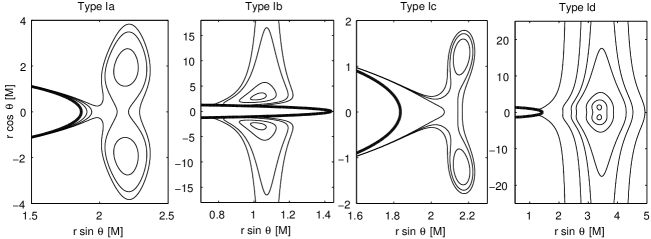
Figure 1: Classification of possible topologies of off-equatorial potential lobes appearing above the event horizon (bold line) of the Kerr black hole immersed into the Wald’s test field. See halo2 for details.

The Hamiltonian equations of motion are given in a standard way:

$${\rm d}x^{\mu}/{\rm d}\lambda=\partial\mathcal{H}/\partial\pi_{\mu},\;\;\;\;\;{\rm d}\pi_{\mu}/{\rm d}\lambda=-\partial\mathcal{H}/\partial x^{\mu},$$ (17)

where $\lambda=\tau/m$ denotes the affine parameter and $\tau$ the proper time.

In the case of stationary and axially symmetric systems we immediately identify two constants of motion from the second Hamiltonian equation, namely energy $E$ and angular momentum $L$:

$$\pi_{t}=p_{t}+qA_{t}\equiv-E,\;\;\;\;\pi_{\phi}=p_{\phi}+qA_{\phi}\equiv L.$$ (18)

4.2 Effective potential

We depart from the normalization of the four-momentum

$$g^{\mu\nu}p_{\mu}p_{\nu}=g^{\mu\nu}(\pi_{\mu}-qA_{\mu})(\pi_{\nu}-qA_{\nu})=-m^{2},$$ (19)

which is conserved along the Hamiltonian flow in autonomous systems. In stationary and axially symmetric situation it allows to express the condition for simultaneous turning point in $r$, $\theta$ coordinates, i.e. simultaneous zero points of $u^{r}=p^{r}/m=g^{rr}\pi_{r}/m$ and $u^{\theta}=p^{\theta}/m=g^{\theta\theta}\pi_{\theta}/m$. These points connect in curves which represent natural boundary for the test particle motion at given energetic level. This two-dimensional (i.e. related to the motion in two coordinates) effective potential describing the motion of the charged test particle takes the following form:

$$V_{\rm eff}(r,\theta;\;a,\>\tilde{q}\tilde{Q},\>\tilde{q}B_{0},\>\tilde{L})=\frac{-\beta+\sqrt{\beta^{2}-4\alpha\gamma}}{2\alpha},$$ (20)

denoting

$$\alpha=-g^{tt},$$ (21)

$$\beta=2[g^{t\phi}(\tilde{L}-\tilde{q}A_{\phi})-g^{tt}\tilde{q}A_{t}],$$ (22)

$$\gamma=-g^{\phi\phi}(\tilde{L}-\tilde{q}A_{\phi})^{2}-g^{tt}\tilde{q}^{2}A_{t}^{2}+2g^{t\phi}\tilde{q}A_{t}(\tilde{L}-\tilde{q}A_{\phi})-1,$$ (23)

where we introduce ”specific” quantities $\tilde{L}\equiv{}L/m$ and $\tilde{q}\equiv{}q/m$. Setting the specific energy $\tilde{E}\equiv{}E/m$ of the given test particle we obtain isocontours forming the boundary of allowed region which is accessible to its trajectory. Since the quantities $\tilde{q}$, $\tilde{Q}$ and $B_{0}$ appear only in terms $\tilde{q}\tilde{Q}$ and $\tilde{q}B_{0}$ we only need to specify values of these two products to uniquely determine the test particle (provided that remaining parameters are already set).

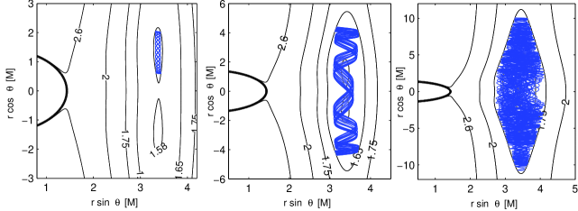
Figure 2: The test particle ($\tilde{L}=6M$, $\tilde{q}B_{0}=M^{-1}$ and $\tilde{q}\tilde{Q}=1$) is launched from the locus of the off-equatorial potential minima $r(0)=3.68\;M$, $\theta(0)=1.18$ with $u^{r}(0)=0$ and various values of the energy $\tilde{E}$. In the left panel we set $\tilde{E}=1.58$ and we observe ordered off-equatorial motion. For the energy of $\tilde{E}=1.65$ cross-equatorial regular motion is observed (middle panel). The trajectory occupies only a part of allowed potential lobe, regardless the length of the integration period. Finally in the right panel with $\tilde{E}=1.75$ we observe irregular motion whose trajectory would ergodically fill whole allowed region after the sufficiently long integration time. We show that the motion is chaotic in this case. Spin of the black hole is $a=0.9\>M$ and its event horizon is depicted by the bold line.

In order to locate the halo orbit and related off-equatorial potential lobe we search for the local minima of the potential $V_{\rm eff}$. Direct approach based on the investigation of the conditions $\frac{\partial{}V_{\rm eff}}{\partial{}r}=0$, $\frac{\partial{}V_{\rm eff}}{\partial\theta}=0$ and the determinant of the Hessian matrix being positive, leads to the set of very intricate algebraic equations. However, when we reformulate these conditions using the force formalism we obtain cubic equation which we are able to solve in general. See kovar08 for details. We found halo2 that potential minima may appear above the event horizon of the black hole, i.e. that off-equatorial stable orbits are allowed in this setup – see Fig. 1. Besides the off-equatorial lobes the potential may form another remarkable structure – endless potential valley of almost constant depth which runs parallelly to the symmetry axis. Thus the particle may escape to infinity from the equatorial plane if its parameters are suitably chosen. Such orbits may form highly collimated jet-like structure and may also provide a charge separation mechanism as was recently reported in preti . Motion in the potential valleys we further discuss in halo3 . Here we concern ourselves with the motion in the closed potential lobes only.

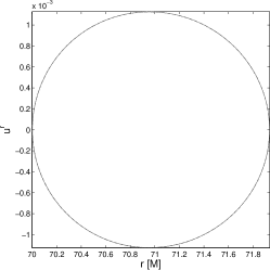
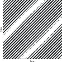
Figure 3: For the sake of comparison we present the surface of section and recurrence plot for a regular trajectory in the fully integrable system of charged test particle ($\tilde{E}=0.9965$, $\tilde{L}=6M$, $\tilde{q}=10^{17}$, $r(0)=70\>M$, $\theta(0)=\theta_{\rm section}=\pi/2$ and $u^{r}(0)=0$) in the pure Kerr-Newman spacetime ($\tilde{Q}=5\times 10^{-18}$, $a=0.9\>M$) endowed with the fourth Carter’s constant of motion $\mathcal{L}$ mtw . Long diagonals parallel to the LOI are a general hallmark of regularity in the RPs.

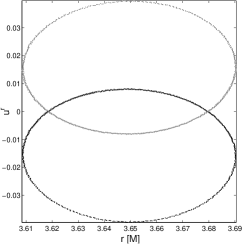
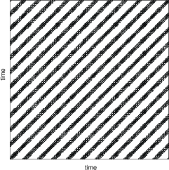
Figure 4: Regular off-equatorial motion of the charged test particle ($\tilde{E}=1.578$, $L=6M$, $\tilde{q}\tilde{Q}=1$, $\tilde{q}B_{0}=M^{-1}$, $r(0)=3.68M$, $u^{r}(0)=0$ and $\theta(0)=\theta_{\rm section}=1.18$) on the Kerr background ($a=0.9\>M$) with the Wald’s test field. In the Poincaré surface of section we distinguish $u^{\theta}\geq 0$ (black point) from $u^{\theta}<0$ (grey point).

5 Regular and chaotic motion in off-equatorial lobes

In this section we shall apply above described recurrence analysis to the chosen set of orbits. From our classification of the off-equatorial potential lobes halo2 which may appear above the horizon of the Kerr black hole immersed in the asymptotically uniform magnetic field (setup described by equations (1), (3) and (4)) we choose the type Id from Fig. 1 for our analysis. In this case the off-equatorial local minima of the effective potential (20) are surrounded by the potential lobes which merge through the equatorial plane once the energy level of the equatorial saddle point is reached and form closed lobe which extends symmetrically above and below the equatorial plane. Increasing the energy even more we would eventually reach the level when this lobe breaks symmetrically in its bottom and upper parts allowing, in principle, the particle to escape to the infinity in the axial direction. Further increase in the energy leads to the opening of the lobe towards the event horizon through the saddle point in the equatorial plane. Described situation is captured in Fig. 2.

Numerical integration of the Hamilton’s equations (17) is carried out using the multistep Adams-Bashforth-Moulton solver of variable order. In several cases when higher accuracy is demanded we employ 7-8th order Dormand-Prince method. Initial values of non-constant components of the canonical momentum $\pi_{r}(0)$ and $\pi_{\theta}(0)$ are obtained from $u^{r}(0)$ (which we set) and $u^{\theta}(0)$ which is calculated from the normalization condition $g^{\mu\nu}u_{\mu}u_{\nu}=-1$ where we always choose the non-negative root as a value of $u^{\theta}(0)$. CRP ToolBox is used for the construction of RPs and evaluation of RQA measures.

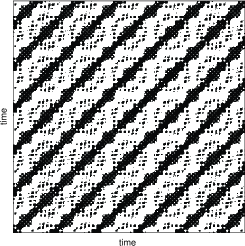
Figure 5: Regular cross-equatorial motion of the charged test particle exposed to the Wald’s field which only differs from the previous case of Fig. 4 by increasing energy to $\tilde{E}=1.65$ for which both off-equatorial potential lobes are already merged via the equatorial plane.

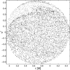
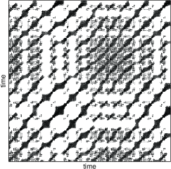
Figure 6: Chaotic motion of the test particle which appears when the energy increases to $\tilde{E}=1.75$ (while all other parameters are kept at values of Figs. 4 and 5).

In Fig. 3 we show how does the regular trajectory in the fully integrable system of the charged test particle in the Kerr-Newman spacetime appear in the Poincaré surface of section and in the recurrence plot. We observe that in this case the RP exhibits purely diagonal features as expected.

Then in Fig. 4 we turn attention to our non-integrable system of the charged test particle being exposed to the Wald’s field on the Kerr background. At given energy level of $\tilde{E}=1.578$ the particle remains trapped in the off-equatorial lobe. Its motion is regular and diagonal structures in the RP typical for the trajectories in integrable systems are preserved, though the pattern is slightly different.

Increasing the energy to $\tilde{E}=1.65$ we obtain the lobe already merged via the equatorial plane. To some surprise the merging itself which occurs at $\tilde{E}\approx 1.59$ is not reflected by the change of the dynamic regime – although the test particle can newly cross the equatorial plane, its motion remains regular (see Fig. 5). Nevertheless the RP proves its dynamics to be more complex than that of the integrable system of Fig. 3. Diagonal structures are preserved, though the pattern is more complicated.

However, at $\tilde{E}=1.75$ we obtain typical chaotic motion Fig. 6. In the surface of section we observe that the trajectory fills all allowed region (hypersurface given by the values of integrals of motion). Diagonal lines in the RP are seriously disrupted and complex large scale structures appear which are characteristic indications of deterministic chaos.

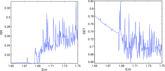
Figure 7: RQA measures $RR$ and $DET$ as a function of specific energy $\tilde{E}$. Dramatic change of behaviour is apparent for both quantities at $\tilde{E}\approx 1.685$. This is where the chaos sets on.

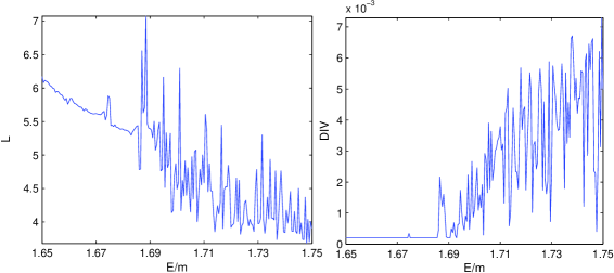
Figure 8: Diagonal RQA measures $L$ and $DIV$ as a function of specific energy $\tilde{E}$. Apparent change of behavior at $\tilde{E}\approx 1.685$ signalizes the onset of chaos.

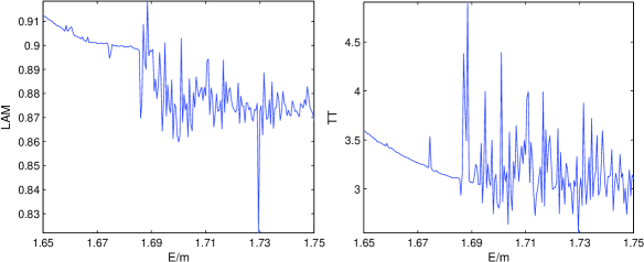
Figure 9: RQA measures derived from vertical lines $LAM$ and $TT$ also clearly signalize the onset of chaos at $\tilde{E}\approx 1.685$.

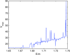
Figure 10: Length of the longest vertical line $V_{\rm{max}}$ generally rises and begins to fluctuate strongly as the chaos sets on at $\tilde{E}\approx 1.685$.

We conclude that the motion in purely off-equatorial lobes (i.e. before merging of the lobes via equatorial plane) is regular. Surprisingly the regularity of motion is not violated when the lobes merge and volume of the accessible portion of phase space suddenly doubles. However, increasing further the energy eventually brings the system to the chaotic regime of motion. This route to chaos was documented by both the standard Poincaré surfaces of section and the recurrence plots. RPs prove to act as an alternative tool to surfaces of section as they allow to distinguish between the regular and the chaotic regime of motion by apparent changes in their patterns.

So far we know that in our set of orbits the transition between the regular and the chaotic regime of the motion occurs somewhere in the range $\tilde{E}\in(1.65,1.75)$. Qualitative methods based on the visual survey of the Poincaré surfaces of section and the recurrence plots do not allow to localise this transition. To this end we employ recurrence quantification analysis (RQA) and observe the behaviour of RQA measures (definitions (8)-(15)). We calculate 200 trajectories with energies equidistantly spread over the range $\left<1.65,1.75\right>$ while other parameters of the system are fixed at values used in Figs. 4–6. In Figs. 7-10 we observe that all queried RQA measures exhibit sudden change in its behaviour at $\tilde{E}\approx 1.685$. This is where the dynamic transition between the regimes occurs. Transition from the regular motion to the chaos is thus detected not only by diagonal RQA measures but also by the vertical ones.

6 Conclusions

In this contribution we demonstrated that the recurrence plots and the recurrence quantification analysis are simple, yet powerful tools which allow one not only to decide whether the dynamic regime of motion is regular or chaotic but also to locate (in terms of some control parameter – energy $\tilde{E}$ in our case) the transition between these regimes with a good precision. General relativistic context highlights the advantages of the recurrence analysis over standard methods as it operates ”locally” (on the small length scale of $\varepsilon$) which allows for various profound computational simplifications when evaluating distances in the phase space. Complex treatment which involves evaluation of the geodesic line and measuring its length may thus be avoided. Major drawback (cost we pay for its simplicity) of RPs and RQA is the lack of invariance (dependence on the threshold $\varepsilon$, $l_{\rm{min}}$, $v_{\rm{min}}$ , choice of the norm etc.). We conclude that RPs themselves may act as an alternative tool to Poincaré surfaces of section and RQA measures are able to detect the transitions between the dynamic regimes.

References

- (1) Kopáček, O., Karas, V., Kovář, J., Stuchlík, Z.: Transition from Regular to Chaotic Circulation in Magnetized Coronae near Compact Objects, Astrophysical Journal, 722, 1240-1259, 2010
- (2) Kovář, J., Kopáček, O., Karas, V., Stuchlík, Z.: Off-equatorial orbits in strong gravitational fields near compact objects – II Classical and Quantum Gravity, 27, 135006-+, 2010
- (3) Kovář, J., Stuchlík, Z. and Karas, V.: Off-equatorial orbits in strong gravitational fields near compact objects Classical and Quantum Gravity, 25, 095011, 2008
- (4) Wald, R. M.: Black hole in a uniform magnetic field, Physical Review D, 10, 1680, 1974
- (5) Marwan, N., Carmen Romano, M., Thiel, M., Kurths, J.: Recurrence plots for the analysis of complex systems, Physics Reports, 438, 237-329, 2007
- (6) Misner C. W., Thorne K. S. and Wheeler J.A.: Gravitation, Freeman, San Francisco, 1973
- (7) Skokos Ch.: The Lyapunov Characteristic Exponents and Their Computation, Lecture Notes in Physics, 790, 63-135, 2010
- (8) Eckmann, J. P., Oliffson Kamphorst, S., Ruelle, D.: Recurrence plots of dynamical systems, Europhysics Letters, 5, 973-977, 1987
- (9) Thorne, K. S., MacDonald, D.: Electrodynamics in Curved Spacetime - 3+1 Formulation, Monthly Notices of the Royal Astronomical Society, 198, 339, 1982
- (10) Bardeen, J. M., Press, W. H. and Teukolsky S. A.: Rotating Black Holes: Locally Nonrotating Frames, Energy Extraction, and Scalar Synchrotron Radiation, Astrophysical Journal, 178, 347-370, 1972
- (11) Thiel, M., Romano, M .C., Kurth J.: How much information is contained in a recurrence plot?, Physics Letters A,330, 343-349, 2004
- (12) Trulla, L. L., Giuliani, A., Zbilut, J. P., Webber, Jr., C. L.: Recurrence quantification analysis of the logistic equation with transients, Physics Letters A, 223, 255-260, 1996
- (13) Preti G.: Nonequatorial charged particle confinement around Kerr black holes 2010 Physical Review D, 81, 024008, 2010