Anisotropic spin Hall effect from first principles

Abstract

We report on first principles calculations of the anisotropy of the intrinsic spin Hall conductivity (SHC) in nonmagnetic hcp metals and in antiferromagnetic Cr. For most of the metals of this study we find large anisotropies. We derive the general relation between the SHC vector and the direction of spin polarization and discuss its consequences for hcp metals. Especially, it is predicted that for systems where the SHC changes sign due to the anisotropy the spin Hall effect may be tuned such that the spin polarization is parallel either to the electric field or to the spin current.

Despite its relative smallness, the spin-orbit interaction (SOI) in solids gives rise to many phenomena of technological relevance and general scientific interest – well-known examples are magnetocrystalline anisotropy and anisotropic magnetoresistance. The anomalous part of the Hall effect Nagaosa et al. (2010), which is observed in ferromagnets even in the absence of a magnetic induction field, results from the spin-dependent transverse velocities which charge carriers acquire in the presence of a longitudinal electric field due to SOI. In paramagnets the spin-dependent transverse velocities of spin-up and spin-down electrons are exactly opposite generating a transverse pure spin current, which is known as spin Hall effect (SHE) D’yakonov and Perel’ (1971); Hirsch (1999); Murakami et al. (2003); Sinova et al. (2004). From the theoretical point of view SHE and anomalous Hall effect (AHE) are thus intimately related and new insights into one of the two effects usually improve understanding of the other.

While the SHE had been predicted theoretically already in 1971 D’yakonov and Perel’ (1971) it was demonstrated experimentally for the first time in 2004 Kato et al. (2004). Since then the enthusiasm about the SHE has not abated. It has been studied experimentally in semiconductors Kato et al. (2004); Sih et al. (2005); Wunderlich et al. (2005); Stern et al. (2006) and metals Valenzuela and Tinkham (2006). As the SHE allows to access the spin degree of freedom of the electron without making use of magnetism it is believed to play an important role in future generations of spintronic devices.

It is well known both from theory and experiment (see Ref. Roman et al. (2009) and references therein) that the anomalous Hall conductivity exhibits anisotropy, i.e., it is dependent on the orientation of magnetization ${\bf{M}}$. Experimental evidence for the anisotropy of the SHE has been reported for AlGaAs quantum wells Sih et al. (2005). In contrast to the AHE the SHE is isotropic in cubic materials, i.e., in order to observe the anisotropy of the SHE non-cubic materials have to be considered Chudnovsky (2009). Besides bearing potential for applications the anisotropic Hall effects are also interesting from the point of view of information encoded in them about the Fermi surfaces and mean free paths of metals. Furthermore, it has been proposed Chudnovsky (2009) to exploit the anisotropy in order to distinguish experimentally between inverse spin Hall effect and competing effects caused by the magnetic field of the transport current. So far, ab initio calculations of the anisotropy of SHE have not been discussed in the literature.

In the present work we undertake a detailed study of the anisotropy of the SHE in nonmagnetic hcp metals and in antiferromagnetic Cr. In particular, the general expression for the orientational dependence of the SHC in hcp and tetragonal metals is derived and the anisotropies are calculated from ab initio within the density functional theory. Generally, in antiferromagnets the SHE is expected to allow the generation of pure spin currents like in paramagnets. While the AHE has recently been studied in complex magnetic structures Yi et al. (2009) first principles calculations of the SHE have been limited to paramagnets so far. Since the magnetic structure breaks the cubic symmetry antiferromagnets such as Cr always exhibit anisotropic SHE.

The anisotropy of the AHE manifests itself in the dependency of the magnitude of the conductivity vector on the magnetization direction. The conductivity vector ${\bm{\sigma}}^{\text{AHE}}({\bf{M}})$ relates the anomalous Hall current density ${\bf{J}}^{\text{AHE}}$ to the electric field:

$${\bf{J}}^{\text{AHE}}={\bf{E}}\times{\bm{\sigma}}^{\text{AHE}}({\bf{M}}).$$ (1)

While the anomalous Hall current is always perpendicular to the electric field, it is not necessarily perpendicular to the magnetization, since conductivity and magnetization vectors are not parallel in general. In the case of the SHE in paramagnets there is no magnetization vector ${\bf{M}}$ to control, only the direction of the applied electric field can be varied. However, the spin polarization of the induced spin current depends on the direction in which the spin current is measured (see Fig. 1(a)). Hence, for a fixed electric field a given spin polarization $\hat{{\bf{S}}}$ is measured only in a certain direction. Thus, in analogy to Eq. (1) we may write

$${\bf{Q}}^{\hat{{\bf{S}}}}={\bf{E}}\times{\bm{\sigma}}(\hat{{\bf{S}}}),$$ (2)

where ${\bf{Q}}^{\hat{{\bf{S}}}}$ is the spin current density and ${\bm{\sigma}}(\hat{{\bf{S}}})$ is the SHC vector. If the magnitude of the SHC vector depends on the spin polarization direction $\hat{{\bf{S}}}$ the SHE is said to be anisotropic.

The spin current is characterized by velocity and spin polarization. Hence, the spin current density ${\bf{Q}}$ is a tensor in the 9-dimensional space $\mathbb{R}^{3}\otimes\mathbb{R}^{3}$ spanned by the basis vectors $\hat{{\bf{e}}}_{i}\otimes\hat{{\bf{s}}}_{s}$. For clarity we use the symbols $\hat{{\bf{s}}}_{x},\hat{{\bf{s}}}_{y}$ and $\hat{{\bf{s}}}_{z}$ to denote the unit vectors of spin polarization while $\hat{{\bf{e}}}_{x}$, $\hat{{\bf{e}}}_{y}$ and $\hat{{\bf{e}}}_{z}$ are the unit vectors of velocity. In addition to the SHC vector we define the tensor of SHC $\sigma_{ij}^{s}$, which has three indices: $i$ denotes the direction of spin current, $j$ the direction of applied external electric field, and $s$ the direction of spin polarization of the spin current. The general expression for the linear response of the spin current density to an applied external electric field is given by

$${\bf{Q}}=\sum_{ijs}\sigma_{ij}^{s}\hat{{\bf{e}}}_{i}\otimes\hat{{\bf{s}}}_{s}E_{j}.$$ (3)

Comparing Eq. (2) and Eq. (3) we find that the SHC vector ${\bm{\sigma}}(\hat{{\bf{S}}})$ and the SHC $\sigma_{ij}^{s}$ are related as follows:

$$\sigma_{k}(\hat{{\bf{S}}})=\frac{1}{2}\sum_{ijs}\epsilon_{ijk}\sigma_{ij}^{s}S_{s},$$ (4)

where $\sigma_{k}$ is the $k$-th component of the conductivity vector, $\hat{{\bf{S}}}=(S_{x},S_{y},S_{z})^{T}$ and $\epsilon_{ijs}$ is the Levy-Civita symbol. Eqns. (3-4) prove Eq. (2), which we conjectured above from analogy to Eq. (1).

In cubic systems symmetry requires that $\sigma_{ij}^{s}=\sigma_{xy}^{z}\epsilon_{ijs}$. Thus, the SHC may be expressed in terms of one material parameter, Eq. (2) simplifies into ${\bf{Q}}^{\hat{{\bf{S}}}}=\sigma_{xy}^{z}{\bf{E}}\times\hat{{\bf{S}}}$, and the conductivity vector is ${\bm{\sigma}}(\hat{{\bf{S}}})=\sigma_{xy}^{z}\hat{{\bf{S}}}$. Since the magnitude of the conductivity vector, $\sigma_{xy}^{z}$, is independent of $\hat{{\bf{S}}}$, the SHE is isotropic in cubic systems. The relationship between the direction of spin current and the direction of spin polarization in cubic systems is illustrated in Fig. 1(a).

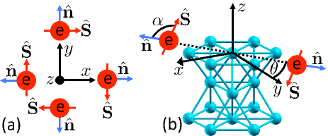
Figure 1: (a) Spin currents in cubic systems induced by an electric field in $z$-direction. For electrons e moving in $y$-direction the spin polarization $\hat{{\bf{S}}}$ points in $x$-direction, while for electrons going in $x$-direction the spin points in minus $y$-direction. (b) Hexagonal hcp structure of the transition metal Ti. Due to the electric field in $x$-direction a spin current flows along $\hat{{\bf{n}}}=(0,\cos\theta,\sin\theta)^{T}$. In general $\hat{{\bf{n}}}$ and $\hat{{\bf{S}}}$ enclose an angle $\alpha\neq 90^{\circ}$.

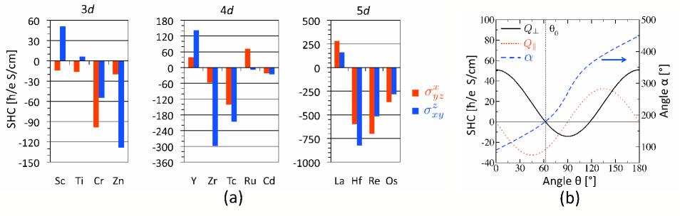
Figure 2: (a) For the hcp metals Sc, Ti, Zn, Y, Zr, Tc, Ru, Cd, La, Hf, Re and Os and for antiferromagnetic Cr the spin Hall conductivities $\sigma^{x}_{yz}$ and $\sigma^{z}_{xy}$ are shown as light (red) and dark (blue) bars, respectively. (b) Decomposition of the SHC of Sc into perpendicular and parallel components following Eq. (6). The angle $\alpha$ enclosed by the direction of the spin current and the direction of the spin polarization is also shown. At the angle $\theta_{0}$=62.2^∘ the component of the spin polarization perpendicular to the spin current vanishes and $\alpha$=180^∘.

In contrast to cubic systems the SHE in hexagonal systems is anisotropic. Consider the structure of the hcp transition metals, which is illustrated in Fig. 1(b). If the electric field is applied along the $x$-direction, the magnitude of the spin current in $y$-direction will generally differ from the one in $z$-direction since the $x$-axis exhibits only 2-fold rotational symmetry. The spin current density in direction $\hat{{\bf{n}}}=(0,\cos\theta,\sin\theta)^{T}$ is

$$\hat{{\bf{n}}}\cdot{\bf{Q}}=-(\sigma^{z}_{xy}\hat{{\bf{s}}}_{z}\cos\theta-\sigma^{y}_{zx}\hat{{\bf{s}}}_{y}\sin\theta)E_{x}.$$ (5)

Note that according to Eq. (3) $\hat{{\bf{n}}}\cdot{\bf{Q}}$ is a vector pointing in the direction of spin polarization. We define the anisotropy of the SHE for spin polarization in the $yz$-plane as $\Delta_{zy}=\sigma_{xy}^{z}-\sigma_{zx}^{y}$. For a general angle $\theta$ the components of the spin current with spin polarization parallel to $\hat{{\bf{n}}}$ ($Q_{\|}$) and spin polarization perpendicular to $\hat{{\bf{n}}}$ ($Q_{\perp}$) are given by

$$Q_{\|} =\hat{{\bf{n}}}\cdot{\bf{Q}}\cdot\hat{{\bf{n}}}=-\frac{1}{2}\Delta_{zy}\sin(2\theta)E_{x},$$ (6)

$$Q_{\perp} =(\sigma_{zx}^{y}+\Delta_{zy}\cos^{2}\theta)E_{x}.$$

If $\Delta_{zy}\neq 0$, the spin polarization is perpendicular to $\hat{{\bf{n}}}$ only if $\hat{{\bf{n}}}$ is along the $y$ or $z$-direction, otherwise spin polarization and direction of spin current enclose the angle $\alpha=\arctan(Q_{\perp}/Q_{\|})\neq 90^{\circ}$, as shown in Fig. 1(b). It follows from Eq. (6) that $Q_{\perp}$ is zero at the angle

$$\theta_{0}=\arccos\sqrt{-\sigma_{zx}^{y}/\Delta_{zy}}$$ (7)

if $\sigma_{xy}^{z}$ and $\sigma_{zx}^{y}$ differ in sign. At this angle $\theta_{0}$ the spin polarization and the spin current are collinear. This is an interesting constellation, which cannot occur in cubic systems.

The case of spin current in $x$-direction and electric field ${\bf{E}}=(0,E\cos\theta,E\sin\theta)^{T}$ in the $yz$-plane is simply related to the previous one by a minus sign: The components of the spin current with spin polarization parallel and perpendicular to the electric field ${\bf{E}}$ are given by $Q_{\|}=\frac{1}{2}\Delta_{zy}\sin(2\theta)E$ and $Q_{\perp}=-(\sigma_{zx}^{y}+\Delta_{zy}\cos^{2}\theta)E_{x}$, respectively. At the angle $\theta_{0}$, Eq. (7), the spin polarization and the electric field are collinear. Thus, one can achieve collinearity of spin polarization and electric field, or collinearity of spin polarization and direction of spin current if $\sigma_{xy}^{z}$ and $\sigma_{zx}^{y}$ differ in sign.

If the electric field is applied along the $z$-axis, the same magnitude of the spin current will be measured in all directions perpendicular to the $z$-axis, since the $z$-axis exhibits 3-fold rotational symmetry. The spin current in direction $\hat{{\bf{n}}}=(\cos\theta,\sin\theta,0)^{T}$ is in this case

$$\hat{{\bf{n}}}\cdot{\bf{Q}}=(\sigma_{yz}^{x}\hat{{\bf{s}}}_{x}\sin\theta-\sigma_{zx}^{y}\hat{{\bf{s}}}_{y}\cos\theta)E_{z}.$$ (8)

Symmetry requires $\sigma_{zx}^{y}=\sigma_{yz}^{x}$. Consequently, the magnitude of the spin current is independent of $\theta$ and the spin polarization is perpendicular to both the electric field and $\hat{{\bf{n}}}$.

In the case of the hcp structure the conductivity vector and the spin current density, Eq. (2), may be expressed in terms of the anisotropy as

$${\bm{\sigma}}(\hat{{\bf{S}}}) =\sigma_{yz}^{x}\hat{{\bf{S}}}+(0,0,\Delta_{zy}S_{z})^{T},$$ (9)

$${\bf{Q}}^{\hat{{\bf{S}}}} =\sigma_{yz}^{x}{\bf{E}}\times\hat{{\bf{S}}}+\Delta_{zy}S_{z}(E_{y},-E_{x},0)^{T}.$$

Hence, only two parameters, $\sigma_{yz}^{x}$ and $\Delta_{zy}$, suffice to describe the SHE in hcp nonmagnetic metals. This is a major difference to the anomalous Hall effect, where four parameters are needed in the phenomenological expansion Roman et al. (2009) of the conductivity of hcp crystals up to third order in the direction cosines, because the band energies depend on the direction of magnetization. Note that Eqns. (5-9) apply also to tetragonal metals.

For the sake of completeness we remark that the analog of Eq. (1) and Eq. (2) runs ${\bf{J}}^{\text{OHE}}={\bf{E}}\times{\bm{\sigma}}^{\text{OHE}}({\bf{B}})$ in the case of the low field ordinary Hall effect (OHE) in paramagnets, where ${\bf{B}}$ is the magnetic induction and ${\bm{\sigma}}^{\text{OHE}}({\bf{B}})=\sigma_{yz}^{x}{\bf{B}}+(0,0,\Delta_{zy}B_{z})^{T}$ is the conductivity vector in hexagonal and tetragonal systems (cf Eq. (9)).

In general there is an intrinsic (independent of impurities) and an extrinsic (impurity-driven) contribution to the SHC (see Ref. Nagaosa et al. (2010) and references therein for the origin of AHE, SHE is analogous). In the first principles calculations of the SHC presented below we consider only the intrinsic Murakami et al. (2003); Sinova et al. (2004); Yao and Fang (2005); Guo et al. (2008) contribution to the SHC, which results from the virtual interband transitions in the presence of an external electric field, and which may be written as a Kubo formula:

$$\sigma_{ij}^{s} =e\hbar\int\frac{d^{3}k}{(2\pi)^{3}}\sum_{n=1}^{N_{\text{occ}}}\Omega_{n}^{s}({\bf{k}}),$$ (10)

$$\Omega_{n}^{s}({\bf{k}}) =2\Im\sum_{n\neq m}\frac{\langle\psi_{{\bf{k}}n}|Q_{i}^{s}|\psi_{{\bf{k}}m}\rangle\langle\psi_{{\bf{k}}m}|v_{j}|\psi_{{\bf{k}}n}\rangle}{(\varepsilon_{n}-\varepsilon_{m})^{2}},$$

where $v_{j}$ is the $j$-component of the velocity operator, $Q_{i}^{s}$ is the spatial $i$- and spin $s$-component of the spin current density operator, $N_{\text{occ}}$ is the number of occupied states, $|\psi_{{\bf{k}}n}\rangle$ is the Bloch function of band $n$ at $k$-point ${\bf{k}}$ and $\varepsilon_{n}$ is its energy eigenvalue. If only the spin conserving part of SOI is taken into account the spin current density operator may be written as $Q_{i}^{s}=\hbar/2\,v_{i}\tau_{s}$. Here, $\tau_{s}$ is a Pauli matrix used to express the $s$-component of the spin operator. In order to treat the spin-nonconserving part of the SOI correctly we used the definition of the spin current density operator given in Ref. Shi et al. (2006).

To disentangle the intrinsic and extrinsic contributions to the SHC experimentally is still a challenge. The anisotropy of the extrinsic AHE is expected to be much smaller than the one of the intrinsic AHE Roman et al. (2009). Since AHE and SHE are analogous concerning their intrinsic and extrinsic mechanisms, also the anisotropy of the extrinsic SHE is expected to be small. Thus, the direct comparison between the experimentally measured anisotropy of the SHC and the one calculated theoretically based on Eq. (10) allows to assess whether the first principles calculations predict the intrinsic contribution to the SHC quantitatively correctly for a given system. If quantitative agreement is found this provides a strong justification for the common procedure to attribute the difference between the experimentally measured SHC and Eq. (10) to extrinsic effects, for the calculation of which ab initio methods have been developed recently Lowitzer et al. (2010); Gradhand et al. (2010, 2010).

Our calculations of the intrinsic SHC, Eq. (10), for the hcp metals Sc, Ti, Zn, Y, Zr, Tc, Ru, Cd, La, Hf, Re and Os and for antiferromagnetic Cr are based on the density functional theory and were performed with the full-potential linearized augmented-plane-wave (FLAPW) code FLEUR fle . The generalized gradient approximation of the exchange correlation potential, a plane-wave cutoff of $K_{\text{max}}=3.7$ bohr^-1, and the experimental lattice constants of the metals were chosen. In the case of Cr we neglected the spin-density wave and considered the antiferromagnetic structure with two atoms in the unit cell and with the magnetic moments parallel and antiparallel to the $z$-axis. A dense $k$-mesh is needed to perform the Brillouin-zone integration in Eq. (10) accurately. Consequently, we made use of Wannier interpolation Wang et al. (2006); Yates et al. (2007) in order to reduce the computational cost. For this purpose we constructed a set of 36 maximally localized FLAPW Wannier functions for each of the metals using the Wannier90 code (see Ref. Mostofi et al. (2008) and references therein) and our interface Freimuth et al. (2008) between FLEUR and Wannier90.

The resulting SHCs are shown in Fig. 2(a). Except for Cd all metals studied in this work exhibit a large anisotropy of SHE, which we expect to be clearly visible in experiments. Of particular interest are the hcp metals Sc, Ti and Ru, where the sign of the conductivity changes as the spin polarization is rotated from the $z$-axis into the $xy$-plane. As discussed before, collinearity of the spin polarization and the electric field (of the spin polarization and the spin current) may be achieved if the electric field (the spin current) lies in the $yz$-plane at the angle $\theta_{0}$, Eq. (7), from the $y$-axis. To illustrate this we plot in Fig. 2(b) the angle $\alpha$ enclosed by the direction of the spin current and the direction of the spin polarization as well as the SHCs associated with $Q_{\|}$ and $Q_{\perp}$ (see Eq. (6)) as a function of the angle $\theta$ for Sc. The critical angles at which the perpendicular component of the spin polarization vanishes are $\theta_{0}$=62.2^∘, $\theta_{0}$=32.1^∘, and $\theta_{0}$=19.1^∘ for Sc, Ti, and Ru, respectively. In the case of Cr the SHE is anisotropic as the cubic symmetry is broken by the staggered magnetization: If the spin polarization of the spin current is perpendicular to the staggered magnetization the SHC is larger by a factor of 1.8 compared to the case of spin polarization parallel to the staggered magnetization.

Generally, the integrand in Eq. (10) varies strongly as a function of ${\bf{k}}$ and the entire Brillouin zone has to be considered in the integration in order to reproduce the SHC quantitatively correctly. This makes it hardly possible to interpret the spin Hall conductivity in terms of a small number of virtual interband transitions. Even the sign and order of magnitude of the SHC are difficult to predict based on simple arguments. Recently, the variation of the sign of the Fermi-surface contribution to the SHC along the 4$d$ and 5$d$ transition metal series has been attributed to the variation of the sign of the spin orbit polarization on the Fermi surface Kontani et al. (2009). However, we find that the spin orbit polarization does not change sign for Sc, Ti and Ru while the SHC changes sign as the spin polarization is rotated from the $z$-axis to the $y$-axis.

In conclusion, we have investigated the dependence of the SHE on the directions of electric field and spin polarization. For the special cases of hexagonal and tetragonal metals we derived the general expression for the SHC vector. We predict that in hcp metals and antiferromagnetic Cr the SHE is strongly anisotropic. For Sr, Ti and Ru the anisotropy is particularly strong since the sign of the SHC depends on the orientation of spin polarization. In this case collinearity of spin polarization and electric field (or spin polarization and spin current) can be achieved for special directions of the electric field (or of the spin current).

We gratefully acknowledge computing time on the supercomputers JUGENE and JUROPA at JSC and funding under the HGF-YIG programme VH-NG-513.

References

- Nagaosa et al. (2010) N. Nagaosa, J. Sinova, S. Onoda, A. H. MacDonald, and N. P. Ong, Rev. Mod. Phys., 82, 1539 (2010).
- D’yakonov and Perel’ (1971) M. I. D’yakonov and V. I. Perel’, JETP Lett., 13, 467 (1971).
- Hirsch (1999) J. E. Hirsch, Phys. Rev. Lett., 83, 1834 (1999).
- Murakami et al. (2003) S. Murakami, N. Nagaosa, and S. C. Zhang, Science, 301, 1348 (2003).
- Sinova et al. (2004) J. Sinova, D. Culcer, Q. Niu, N. A. Sinitsyn, T. Jungwirth, and A. H. MacDonald, Phys. Rev. Lett., 92, 126603 (2004).
- Kato et al. (2004) Y. K. Kato, R. C. Myers, A. C. Gossard, and D. D. Awschalom, Science, 306, 1910 (2004).
- Sih et al. (2005) V. Sih, R. C. Myers, Y. K. Kato, W. H. Lau, A. C. Gossard, and D. D. Awschalom, Nature Phys., 1, 31 (2005).
- Wunderlich et al. (2005) J. Wunderlich, B. Kaestner, J. Sinova, and T. Jungwirth, Phys. Rev. Lett., 94, 047204 (2005).
- Stern et al. (2006) N. P. Stern, S. Ghosh, G. Xiang, M. Zhu, N. Samarth, and D. D. Awschalom, Phys. Rev. Lett., 97, 126603 (2006).
- Valenzuela and Tinkham (2006) S. O. Valenzuela and M. Tinkham, Nature, 442, 176 (2006).
- Roman et al. (2009) E. Roman, Y. Mokrousov, and I. Souza, Phys. Rev. Lett., 103, 097203 (2009).
- Chudnovsky (2009) E. M. Chudnovsky, Phys. Rev. B, 80, 153105 (2009).
- Yi et al. (2009) S. D. Yi, S. Onoda, N. Nagaosa, and J. H. Han, Phys. Rev. B, 80, 054416 (2009).
- Yao and Fang (2005) Y. Yao and Z. Fang, Phys. Rev. Lett., 95, 156601 (2005).
- Guo et al. (2008) G. Y. Guo, S. Murakami, T. W. Chen, and N. Nagaosa, Phys. Rev. Lett., 100, 96401 (2008).
- Shi et al. (2006) J. Shi, P. Zhang, D. Xiao, and Q. Niu, Phys. Rev. Lett., 96, 76604 (2006).
- Lowitzer et al. (2010) S. Lowitzer, D. Ködderitzsch, and H. Ebert, Phys. Rev. B, 82, 140402 (2010).
- Gradhand et al. (2010) M. Gradhand, D. V. Fedorov, P. Zahn, and I. Mertig, Phys. Rev. Lett., 104, 186403 (2010a).
- Gradhand et al. (2010) M. Gradhand, D. V. Fedorov, P. Zahn, and I. Mertig, Phys. Rev. B, 81, 245109 (2010b).
- (20) See http://www.flapw.de.
- Wang et al. (2006) X. Wang, J. R. Yates, I. Souza, and D. Vanderbilt, Phys. Rev. B, 74, 195118 (2006).
- Yates et al. (2007) J. R. Yates, X. Wang, D. Vanderbilt, and I. Souza, Phys. Rev. B, 75, 195121 (2007).
- Mostofi et al. (2008) A. A. Mostofi, J. R. Yates, Y.-S. Lee, I. Souza, D. Vanderbilt, and N. Marzari, Computer Physics Communications, 178, 685 (2008).
- Freimuth et al. (2008) F. Freimuth, Y. Mokrousov, D. Wortmann, S. Heinze, and S. Blügel, Phys. Rev. B, 78, 035120 (2008).
- Kontani et al. (2009) H. Kontani, T. Tanaka, D. S. Hirashima, K. Yamada, and J. Inoue, Phys. Rev. Lett., 102, 016601 (2009).