Multigrid solver for clover fermions

Abstract:

We present an adaptive multigrid Dirac solver developed for Wilson clover fermions which offers order-of-magnitude reductions in solution time compared to conventional Krylov solvers. The solver incorporates even-odd preconditioning and mixed precision to solve the Dirac equation to double precision accuracy and shows only a mild increase in time to solution for decreasing quark mass. We show actual time to solution on production lattices in comparison to conventional Krylov solvers and will also discuss the setup process and its relative cost to the total solution time.

1 Introduction

Much of the work in lattice QCD goes into the repeated solution of Dirac equation

$$\left[D(U)+m\right]\psi=\eta$$ (1)

for varying sources $\eta$ and/or gauge fields $U$. Typically this is done with a Krylov solver such as conjugate gradients (CG) or BiCGStab. These methods are known to exhibit critical slowing down where the time to solution increases rapidly as the quark mass is decreased. This is because the condition number of the Dirac matrix tends to diverge (for a large enough volume) as the mass decreases ($\kappa\sim 1/m$), while standard Krylov solvers become inefficient as the condition number grows (iterations ${}^{>}_{\sim}$$\sqrt{\kappa}$).

A lot of work has been done on developing deflation methods that remove a set of low modes (i.e., eigenvectors with small eigenvalues) from the solver, leading to improvements in the solver time [1]. However all these methods will require deflating a number of modes that scales linearly with the volume, which then becomes more difficult as the volume increases. An alternative is to use the local deflation approach of Lüscher [2] which splits the low vectors into spatial blocks which then gives a larger span of modes to deflate, and thus does not require a number of vectors that scales with volume. This splitting of vectors is similar to that done in multigrid methods [3] which we describe here.

While multigrid methods have been very successful in other fields, their application to lattice QCD has been difficult due to the complexity of the low modes of the QCD Dirac operator. We have been working to apply the methods of adaptive multigrid to QCD starting with plain Wilson quarks in 2d [4] and 4d [5]. Here we present the extension to 4d clover improved Wilson quarks and show results of a production-ready implementation using the USQCD software libraries [6].

Adaptive multigrid: The main motivation behind multigrid is the observation that in typical linear systems (from discretized PDEs) the low modes, which are responsible for the poor convergence of the solver, are smooth and therefore can be approximated well on a coarser grid which reduces the effort required to solve for them. The problem is then essentially split into two parts with the high frequency components being solved on the original (fine) grid and the low modes being solved on a coarse grid. The basic multigrid algorithm consists of alternating between a relaxation step (smoother) on the fine grid using traditional iterative solvers (typically stationary or Krylov) and a solve on a coarse grid. This procedure can be repeated recursively to solve the coarse grid problem, reducing to coarser and coarser grids until the coarsest problem is small enough to be easily solved.

The key components of the algorithm are the choice of smoother and the operators used for the coarse solve: restriction, $R$, used to project the error from the fine lattice onto the coarse; prolongation, $P$, (or interpolation) used to bring the coarse grid correction back up to the fine level; and the coarse operator itself. The multigrid procedure is usually not used on its own and is often used as a preconditioner for another solver. For our application, with a non-Hermitian Wilson Dirac operator and our choice of a non-stationary multigrid cycle, we use generalized conjugate residuals (GCR) as the outer solver. Since the basic algorithm for Wilson fermions has already appeared in [5], here we will focus on the extensions to that algorithm.

Red-black preconditioning: The common approach to solving for the Wilson Dirac operator on the lattice is to first employ red-black (even-odd) preconditioning which substantially reduces the number of iterations needed to solve the system [7]. We implement this by splitting the linear system, $Dx=b$, into even ($e$) and odd ($o$) space-time sites as

$$\left(\begin{array}[]{cc}D_{ee}&D_{eo}\\ D_{oe}&D_{oo}\\ \end{array}\right)\left(\begin{array}[]{c}x_{e}\\ x_{o}\end{array}\right)=\left(\begin{array}[]{c}b_{e}\\ b_{o}\end{array}\right)\Rightarrow\left(\begin{array}[]{cc}1&D_{eo}D_{oo}^{-1}\\ D_{oe}D_{ee}^{-1}&1\\ \end{array}\right)\left(\begin{array}[]{c}D_{ee}x_{e}\\ D_{oo}x_{o}\end{array}\right)=\left(\begin{array}[]{c}b_{e}\\ b_{o}\end{array}\right)~{}.$$ (14)

The mass term is now absorbed into $D$. In the preconditioned form, $D_{p}y=b$, on the right side of (14), we can solve the reduced system, $D_{r}y_{e}=b_{r}$, with

$$D_{r} = 1-D_{eo}D_{oo}^{-1}D_{oe}D_{ee}^{-1}$$ (15)

$$b_{r} = b_{e}-D_{eo}D_{oo}^{-1}b_{o}~{},$$ (16)

for the even sites, $y_{e}=D_{ee}x_{e}$. The matrices $D_{ee}$ and $D_{oo}$ are diagonal on the space-time lattice so we can easily compute $D_{r}$ and $b_{r}$ and reconstruct $x_{e}=D^{-1}_{ee}y_{e}$ and $x_{o}=D^{-1}_{oo}(b_{o}-D_{oe}x_{e})$.

On the fine level, we use a GCR solver for the reduced system: $D_{r}y_{e}=b_{r}$. However the coarse operator, $\widehat{D}=RD_{p}P$, is a projection of the full even-odd preconditioned matrix ($D_{p}$). When solving the coarse system we again use even-odd preconditioning to solve the reduced coarse system. The interpolation operator ($P$) is formed from the low modes of the the full preconditioned operator $D_{p}$. One can easily see that the eigenvectors of $D_{p}$ and $D_{r}$ are the same on the even sites so that the low modes of the two are related. For the $\gamma_{5}$-Hermitian Wilson Dirac operator, we constructed the restriction operator $R$ using $R=P^{\dagger}\gamma_{5}$. We also split the vectors that formed $P$ into the 2 chiralities in addition to the space-time blocks, explicitly preserving $\gamma_{5}$-Hermiticity on the coarse level and helping to avoid a nearly singular coarse operator. For the Wilson clover case, $D_{p}$ is not $\gamma_{5}$-Hermitian, however we still use the same construction. Initial tests on smaller Wilson lattices found a 30% improvement using the preconditioning, so we have adopted it for clover lattices too.

Implementation: The multigrid solver has been implemented using the US DOE SciDAC lattice QCD libraries [6] and in particular it is written in the C language version of the QCD data parallel layer QDP/C. This library has been extended to provide multi-lattice support and improved arbitrary $N_{c}$ support which is used to implement the coarse level operators (which look similar to a staggered Dirac operator with $N_{c}$ equal to the number of vectors used to form $P$ and $R$).

Since the single precision operations are generally faster than double precision, we have implemented the multigrid preconditioner in single precision while the outer GCR solver is in full double precision. In all cases tested so far, single precision is sufficiently accurate to provide a good preconditioner for the Dirac matrix. For comparison to conventional Krylov solvers below we have also included a mixed precision version of those based on iterative refinement. Other mixed precision methods such as reliable updates [8] may perform better at lighter masses, but we do not expect this to make a large difference in the final results.

In typical multigrid implementations, one has a choice of how many cycles of the coarse solve and smoothing to perform at each level before going back up to the next finer level. These choices include the conventional V-cycle, where no extra cycles are performed, or a W-cycle, where one extra cycle at the coarsest level is performed, or some more sophisticated pattern. Here instead of choosing the pattern up front, we implement the recursive solver in a truly adaptive fashion where the coarse grid solver is again a GCR solver preconditioned with another multigrid cycle, and so on until the coarsest lattice, which is solved with an unpreconditioned GCR. At each level we only specify the residual tolerance for each GCR solver which then lets the solver at each level determine how many cycles are needed to reach the requested tolerance. We ran the multigrid solver with many different sets of parameters and found that a tolerance of around 0.1 is usually best. This means that the coarse solves do not need to be done very accurately. In all results below the times reported were for the best set of parameters found for that particular case.

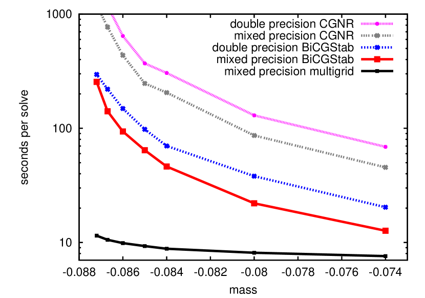
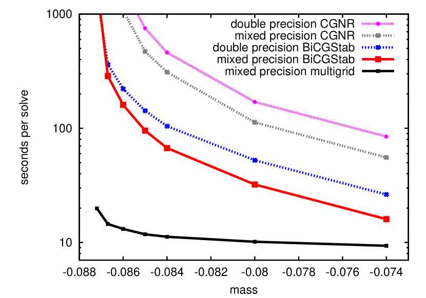
Figure 1: Time to solution (in seconds) for a single solve versus quark mass for various Krylov solvers and multigrid. The left plot is for the $24^{3}\times 128$ lattice and the right is for $32^{3}\times 256$.

2 Results

We have tested the multigrid algorithm on the Hadron Spectrum Collaboration anisotropic clover lattices [9]. We have run on lattices of size $24^{3}\times 128$ and $32^{3}\times 256$ with spatial and temporal lattice spacings of $a_{s}\approx 0.12$ fm and $a_{t}\approx 0.035$ fm. The light dynamical mass ($m_{l}=-0.086$) corresponds to $m_{\pi}\approx 220$ MeV. For reference the strange quark on these lattices was determined to be $m_{s}\approx-0.0743$, while the physical light quark mass would be around $m_{l}\approx-0.0867$. The sizes of the coarse lattices and number of low vectors used in the restriction and prolongation operators are given in table 1. All results were obtained on 256 or 1024 cores of a Blue Gene/P.

lattice	cores	$1^{st}$ coarse lattice	# vectors in $1^{st}$ $P$	$2^{nd}$ coarse lattice	# vectors in $2^{nd}$ $P$
$24^{3}\times 128$	256	$8^{3}\times 16$	24	$4^{3}\times 4$	32
$32^{3}\times 256$	1024	$16\times 8\times 8\times 32$	24	$4^{3}\times 16$	32

Table 1: multigrid parameters

Figure 1 shows the time to solution for a single solve as a function of the quark mass for various solvers for the two lattice volumes. In all cases the conjugate gradients on the normal residual (CGNR) performed worse than BiCGStab and the mixed precision solver performed better than pure double precision. The multigrid solver performs much better than the others and shows a much smaller increase in time as the quark mass is decreased. For the larger volume the speedup factor of multigrid compared to mixed precision BiCGStab is about $1.7\times$ at the heaviest mass, $12.2\times$ at the dynamical light mass and $19.8\times$ at the physical light mass. On the larger volume we see a sharper increase in time at the smallest masses compared to the smaller volume. We expect that this could be improved with additional work in the setup and/or adding a fourth level.

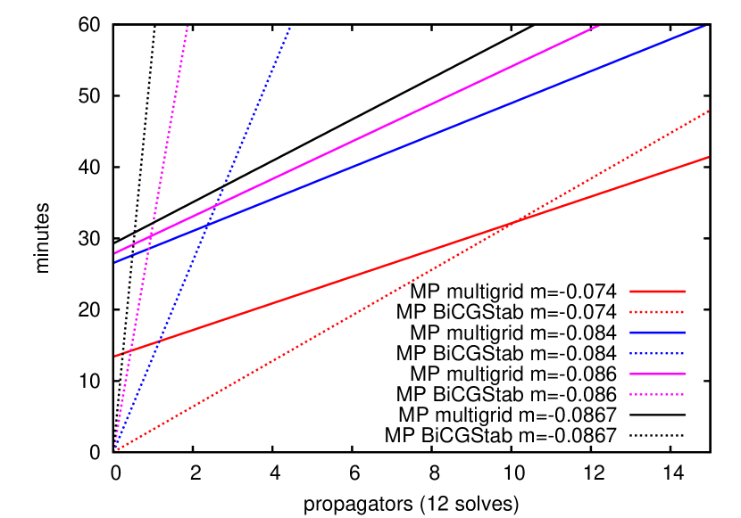
Figure 2: Total time to solution including setup versus number of right hand sides for mixed precision (MP) BiCGStab and multigrid at different quark masses.

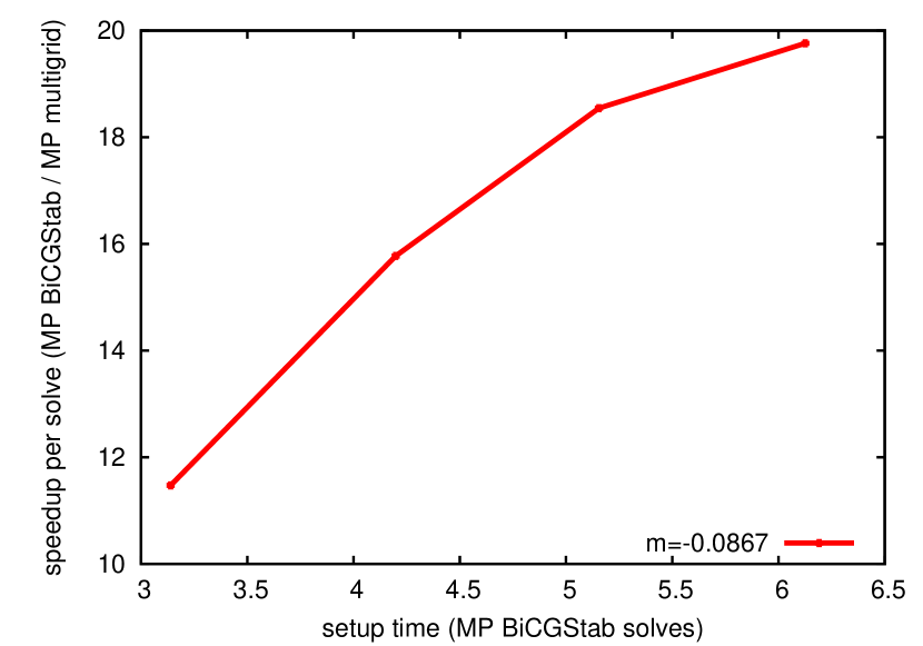
Figure 3: Speedup of multigrid solver relative to BiCGStab versus setup time at the physical quark mass.

In figure 3 we show the total time required to solve different number of right hand sides, including the setup cost, on the larger volume. For small numbers of solves, BiCGStab is faster due to the setup time needed for multigrid. As the number of solves increases multigrid becomes faster due to the improved time per solution. The break even point becomes smaller as the quark mass is decreased. At close to strange quark mass the crossing is at around 10 full propagators (of 12 solves each). At the dynamical mass the crossing is at 1 full propagator and at the physical mass it is about half a propagator (6 solves). Of course it is possible to save the vectors and even the coarse matrix to load back in for later analysis, so for analysis projects on saved configurations, the setup cost should not be an issue. Only for configuration generation is the setup cost an issue. Since the main focus for the implementation is currently for analysis, the setup code has not been fully tuned and there is still room for improvement both algorithmically and in code optimization.

One still has some freedom to choose how much time to spend in the setup procedure which then affects the quality of the resulting solver. In figure 3 we plot the speedup for a single application of the multigrid solver relative to BiCGStab versus the time spent in the setup (in units of the time for a single BiCGStab solve). These results were obtained on the larger lattice at the physical quark mass. If we spend about 6 BiCGStab solves worth of work in the setup we get a solver that is about $20\times$ faster than BiCGStab, which is what was used in the previous figures. If we lower the setup cost to about 3 BiCGStab solves, then the solver speedup reduces to around $11\times$.

We can see how this freedom can be used to optimize the total time in figure 5. Here we show the total solution time including setup versus number of solves for the four different setups shown in the previous figure. These runs were again done on the larger lattice at the physical mass. Here we see that the smallest setup time gives the best total performance up to about 4 propagators at which point the second smallest setup becomes best. The third setup takes over at around 8 propagators and the last at around 25. Thus if the setup is not being saved for reuse at a later time, one can optimize the setup for the particular work being done.

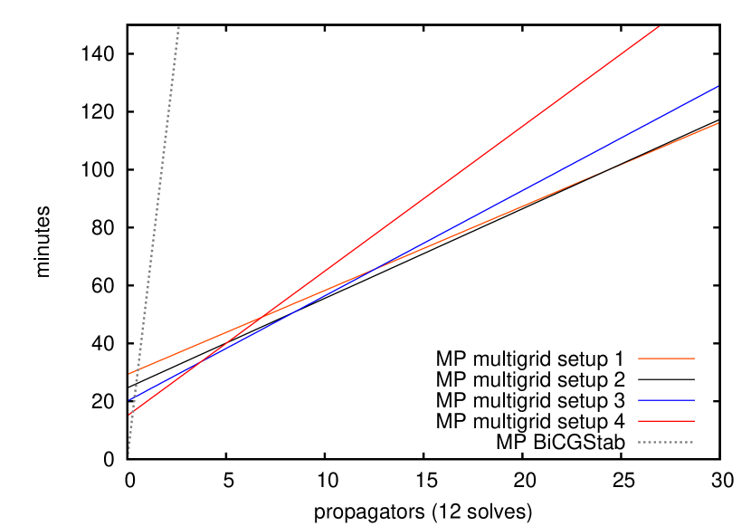
Figure 4: Total time versus number of solves for different amounts of setup work on the $32^{3}\times 256$ lattice at the physical mass.

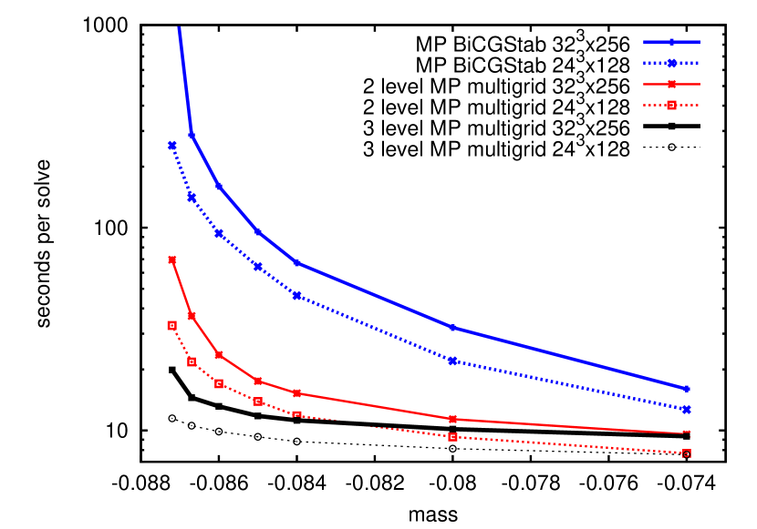
Figure 5: Comparison of 2 and 3 level multigrid algorithms on both lattice sizes.

In figure 5 we compare the performance of the 2-level and 3-level multigrid algorithms for both lattice sizes. For heavier masses the difference between 2 and 3 levels is small while both are still better than BiCGStab. For lighter masses the 3 level algorithm is clearly better and is about $2.5\times$ better at the physical quark mass. As noted earlier the increase in time seen for the 3-level algorithm at the lightest quark masses suggests that improving the coarse level with additional work in the setup and/or adding a fourth multigrid level may be beneficial here.

In figure 7 we show how the relative speedup of multigrid over BiCGStab varies with the requested residual tolerance. These results are obtained at the physical mass. For the smaller volume the speedup appears to stay constant as the tolerance changes, however for the larger volume, the speedup tends to increase as the tolerance is lowered. Thus the multigrid algorithm is even more effective for smaller tolerances.

Although the residual is typically used as the measure of convergence due to it being readily available, what usually matters for observables is the actual error defined by $e=D^{-1}b-x$. It is related to the residual $r$ by $r=b-Dx=De$. Since the residual is the error multiplied by $D$, it is not as sensitive to low modes. In figure 7 we plot the ratio of the magnitude of the error to the magnitude of the residual versus the magnitude of the residual for BiCGStab and multigrid at the physical mass. In order to know the exact solution, we first take a point source ($p$), then solve against that to get an approximate solution $x_{0}\approx D^{-1}p$. We set the right hand side to be $b=Dx_{0}$ so that $b$ is approximately a point source and its exact solution is known. The error is very stable for multigrid and stays at about $40-50\times$ the residual for both lattice volumes. The BiCGStab error fluctuates wildly at about $5-10\times$ larger than the multigrid error and appears to grow with volume.

3 Setup procedure

Currently the setup procedure consists of a sequence of repeated relaxations (inverse iteration) on a random vector, $v$, while monitoring the Rayleigh quotient $v^{\dagger}D^{\dagger}Dv/v^{\dagger}v$ to determine when the vector has converged well enough onto the low modes of the system. During this process we also keep the current vector globally orthogonal to the previously converged vectors. The main motivation for implementing this setup procedure is its simplicity since one doesn’t need to construct coarse operator until all the vectors are found. It is also relatively easy to vary the number of iterations and the convergence criteria to tune the cost of the setup and consequently the efficiency of the resulting solver. However the main drawback of this procedure is that the resulting vectors may be locally redundant within the blocks. More sophisticated setup procedures have been developed to avoid this problem. One such setup procedure is used in the adaptive smooth aggregation ($\alpha$SA) method [10]. Here one constructs a multigrid cycle out of the currently available vectors and uses that solver to relax on random vectors which will then give a new vector which is rich in the modes that the current solver is bad at resolving. This requires construction of coarse operator several times during the setup process which adds to the complexity and possibly also the time of the setup. A hybrid approach combining these procedures was developed for the Wilson case with promising results [5]. We plan to implement this for the clover case in the future.

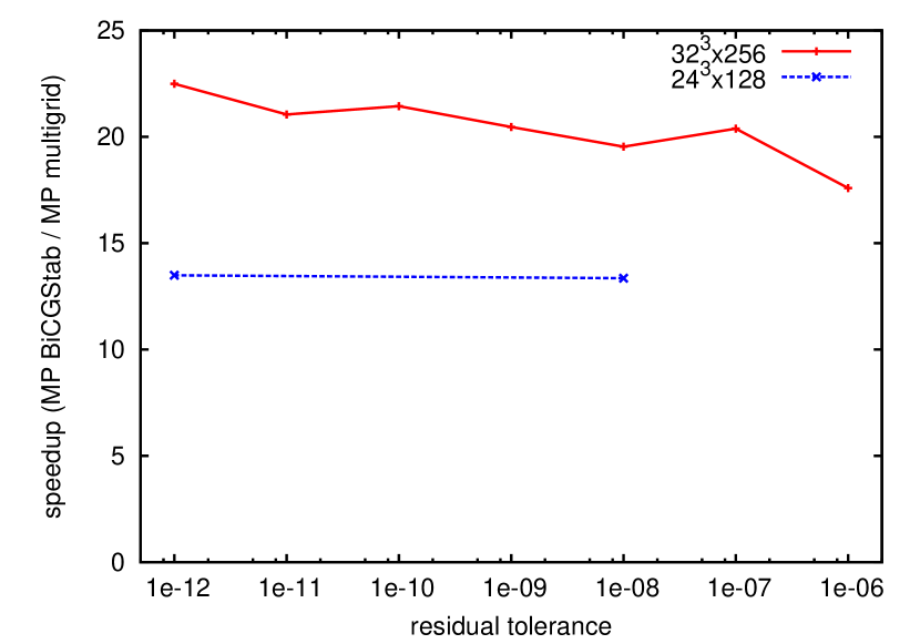
Figure 6: Speedup of multigrid over BiCGStab versus requested residual tolerance. On the larger lattice we see the speedup increase as the tolerance decreases.

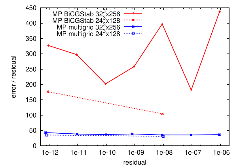
Figure 7: Ratio of magnitude of error to magnitude of residual versus magnitude of residual for BiCGStab and multigrid.

4 Summary and plans

We have developed an efficient implementation of a Wilson clover multigrid solver, currently being used in production for the calculation of disconnected diagrams. For light quarks we see a $10-20\times$ reduction in time to solution. We also note that the error is very stable and relatively small compared to Krylov solvers and that the speedup and relative error improves for larger lattices. We are now in the process of testing it on larger lattices and working on optimizing the code so it can be extended to even coarser lattices. Currently the solver is a great improvement for medium to large analysis projects where the setup cost can be amortized over many solves. We are working to improve the setup process to provide the same or better quality solver and lower cost so that it can be readily used in smaller projects or in configuration generation. Finally we are working on multigrid for domain wall and staggered quarks, as well as porting these solvers to GPUs.

Acknowledgments: This work was supported by the US NSF and DOE. Runs were performed at the Argonne Leadership Computing Facility which is supported under DE-AC02-06CH11357.

References

- [1] R. B. Morgan and W. Wilcox, arXiv:0707.0505 [math-ph]; A. Stathopoulos and K. Orginos, SIAM J. Sci. Comput. 32, 1 (2010).
- [2] M. Lüscher, JHEP 0707, 081 (2007).
- [3] A. Brandt, Math. Comp. 31, 138 (1977).
- [4] J. Brannick, R. C. Brower, M. A. Clark, J. C. Osborn and C. Rebbi, Phys. Rev. Lett. 100, 041601 (2008).
- [5] R. Babich et al., accepted for publication in Phys. Rev. Lett., arXiv:1005.3043 [hep-lat].
- [6] http://usqcd.jlab.org/usqcd-software
- [7] T. DeGrand, Comput. Phys. Commun. 52, 161 (1988).
- [8] M. A. Clark, R. Babich, K. Barros, R. C. Brower and C. Rebbi, Comput. Phys. Commun. 181, 1517 (2010).
- [9] H. W. Lin et al. [Hadron Spectrum Collaboration], Phys. Rev. D 79, 034502 (2009).
- [10] M. Brezina, R. Falgout, S. MacLachlan, T. Manteuffel, S. McCormick and J. Ruge, SIAM J. Sci. Comput. 25, 6 (2004).