On the electrical current distributions for the generalized Ohm’s Law

Abstract

The paper studies a particular class of analytic solutions for the Generalized Ohm’s Law, approached by means of the so called formal powers of the Pseudoanalytic Function Theory. The reader will find a description of the electrical current distributions inside bounded domains, within inhomogeneous media, and their corresponding electric potentials near the boundary. Finally, it is described a technique for approaching separable-variables conductivity functions, a requisite when applying the constructive methods posed in this work.

1 Introduction

The study of the generalized Ohm’s Law

$$\text{div}\left(\sigma\text{grad}u\right)=0,$$ (1)

where $\sigma$ denotes the electrical conductivity function and $u$ is the electric potential, is the base for well understanding a wide class of problems in Electromagnetic Theory, just as the Electrical Impedance Tomography, the name given in medical imaging for the inverse problem posed by Calderon [3] in 1980. Yet, for many decades, the mathematical complexity of (1) imposed so difficult challenges to the researchers, that the structure of its general solution in analytic form remained unknown. It was until 2006 that K. Astala and L. Päivärinta [1] discovered that the two-dimensional case of (1) was closely related with a Vekua equation [15], and in 2007 V. Kravchenko et al. [8], based upon elements of Pseudoanalytic Function Theory [2], achieved to pose what could be considered the first general solution in analytic form of (1) for the plain, when the conductivity function $\sigma$ belongs to a special class of functions.

Virtually, these two discoveries were the departure point for developing a completely new theory for the generalized Ohm’s Law, mainly because they allowed to research a wide sort of electromagnetic phenomena that had remained out of range for the mathematical tools known previously.

In this paper we discuss the possibility of considering the formal powers [2], as a new scope for analyzing the electrical current distributions inside inhomogeneous media in bounded domains, since it is bias their linear combination that we can approach the general solution for the two-dimensional case of (1) [13], and they are also useful for constructing an infinite set of analytic solutions for its three-dimensional case [12].

Starting with the elements of Pseudoanalytic Function Theory, and of Quaternionic Analysis, we briefly expose an idea for rewriting the three-dimensional case of (1) in a quaternionic equation, in order to pose the structure of its general solution by means of a generalization of the Bers generating pair, in Complex Analysis.

Eventually, we focus our attention on the plane by considering one example in which a spacial variable is fixed, and the conductivity $\sigma$ adopts an exponential form. Then we trace the electrical current density patches, obtained from the solutions of the Vekua equation in terms of Taylor series in formal powers, and we show that, from an adequate point of view, the observed patches might keep a sort of regular dynamics when flowing through this inhomogeneous medium, once they are compared to those traced for an homogeneous case.

The work closes with a basic idea for approaching separable-variables conductivity functions, since this is the central requirement if we are to apply the exposed mathematical ideas for approaching solutions of (1), and to analyze their meaning in terms of electrical current flows.

2 Preliminaries

2.1 Elements of pseudoanalytic functions

Following L. Bers [2], a pair of complex-valued functions $F=\text{Re}\left(F\right)+i\text{Im}\left(F\right)$ and $G=\text{Re}\left(G\right)+i\text{Im}\left(G\right)$ will be called a generating pair if the following condition holds:

$$\text{Im}\left(\overline{F}G\right)>0.$$ (2)

Here $i$ denotes the standard imaginary unit $i^{2}=-1$, whereas $\overline{F}$ represents the complex conjugation of $F:\overline{F}=\text{Re}\left(F\right)-i\text{Im}\left(F\right).$ Thus, any complex-valued function $W$ can be represented as the linear combination of the generating pair $\left(F,G\right)$:

$$W=\phi F+\psi G,$$ (3)

where $\phi$ and $\psi$ are both real-valued functions. Hence the derivative in the sense of Bers, or $\left(F,G\right)$-derivative, of a complex-valued function $W$ will be defined as

$$\partial_{\left(F,G\right)}W=\left(\partial_{z}\phi\right)F+\left(\partial_{z}\psi\right)G,$$ (4)

where $\partial_{z}=\frac{\partial}{\partial x}-i\frac{\partial}{\partial y}$, and it will exist if and only if

$$\left(\partial_{\overline{z}}\phi\right)F+\left(\partial_{\overline{z}}\psi\right)G=0,$$ (5)

where $\partial_{\overline{z}}=\frac{\partial}{\partial x}+i\frac{\partial}{\partial y}.$ Notice even the operators $\partial_{z}$ and $\partial_{\overline{z}}$ are usually defined including the coefficient $\frac{1}{2},$ it will result somehow more convenient for this paper to work without it.

By introducing the notations

$$A_{\left(F,G\right)}=-\frac{\overline{F}\partial_{z}G-\overline{G}\partial_{z}F}{F\overline{G}-\overline{F}G},\text{ \ \ }a_{\left(F,G\right)}=-\frac{\overline{F}\partial_{\overline{z}}G-\overline{G}\partial_{\overline{z}}F}{F\overline{G}-\overline{F}G},$$ (6)

$$B_{\left(F,G\right)}=\frac{F\partial_{z}G-G\partial_{z}F}{F\overline{G}-\overline{F}G},\text{ \ \ }b_{\left(F,G\right)}=\frac{F\partial_{\overline{z}}G-G\partial_{\overline{z}}F}{F\overline{G}-\overline{F}G};$$

the $\left(F,G\right)$-derivative of $W$ (4) can be written as

$$\partial_{\left(F,G\right)}W=A_{\left(F,G\right)}W+B_{\left(F,G\right)}\overline{W},$$ (7)

and the condition (5) will turn into

$$\partial_{\overline{z}}W-a_{\left(F,G\right)}W-b_{\left(F,G\right)}\overline{W}=0.$$ (8)

The last differential equation is known as the Vekua equation [15], and it will play a very important roll in our further discussions. The functions defined in (6) are known as the characteristic coefficients of the generating pair $\left(F,G\right)$, and every complex-valued function $W$ satisfying (8) will be referred as an $\left(F,G\right)$-pseudoanalytic function.

The following statements were originally posed in [2]. Another authors will be cited explicitly.

Remark 1

The functions conforming the generating pair $\left(F,G\right)$ are $\left(F,G\right)$-pseudoanalytic, and their $\left(F,G\right)$-derivatives are $\partial_{\left(F,G\right)}F=\partial_{\left(F,G\right)}G=0.$

Remark 2

Let $p$ be a non-vanishing function inside some domain $\Omega$. The pair of functions $F=p$ and $G=\frac{i}{p}$ satisfy the condition (2), so they constitute a Bers generating pair, and their characteristic coefficients are

$$A_{\left(F,G\right)}=a_{\left(F,G\right)}=0,$$ (9)

$$B_{\left(F,G\right)}=\frac{\partial_{z}p}{p},\text{ \ \ }b_{\left(F,G\right)}=\frac{\partial_{\overline{z}}p}{p}.$$

Theorem 1

[6] Let $p$ be a non-vanishing function within some domain $\Omega$. The pair of real-valued functions $\phi$ and $\psi$ will be solutions of the system

$$\frac{\partial}{\partial x}\phi=\frac{1}{p^{2}}\frac{\partial}{\partial y}\psi,\text{ \ \ }\frac{\partial}{\partial y}\phi=-\frac{1}{p^{2}}\frac{\partial}{\partial x}\psi,$$ (10)

if and only if $W=p\phi+\frac{i}{p}\psi$ is solution of the Vekua equation

$$\partial_{\overline{z}}W-\frac{\partial_{\overline{z}}p}{p}\overline{W}=0.$$

A pair of functions $\phi$ and $\psi$ satisfying (10) is called a $p$-analytic system [11].

Definition 1

Let $\left(F_{0},G_{0}\right)$ and $\left(F_{1},G_{1}\right)$ be two generating pairs, and let their characteristic coefficients satisfy

$$a_{\left(F_{0},G_{0}\right)}=a_{\left(F_{1},G_{1}\right)}\text{ \ \ \ and \ \ \ }B_{(F_{0},G_{0})}=-b_{(G_{1},F_{1})}.$$ (11)

The generating pair $\left(F_{1},G_{1}\right)$ will be called a successor pair of $\left(F_{0},G_{0}\right),$ as well as the pair $\left(F_{0},G_{0}\right)$ will be called a predecessor of $\left(F_{1},G_{1}\right)$.

Theorem 2

Let the complex-valued function $W$ be $\left(F_{0},G_{0}\right)$-pseudoanalytic, and let the generating pair $\left(F_{1},G_{1}\right)$ be a successor pair of $\left(F_{0},G_{0}\right)$. Hence, the $\left(F_{0},G_{0}\right)$-derivative of $W$ will be an $\left(F_{1},G_{1}\right)$-pseudoanalytic function.

Definition 2

Let the pairs of functions belonging to the set

$$\left\{\left(F_{n},G_{n}\right):n=0,\pm 1,\pm 2,...\right\}$$ (12)

be all generating pairs, and let every $\left(F_{n+1},G_{n+1}\right)$ be a successor pair of $\left(F_{n},G_{n}\right)$. Then the set (12) is called a generating sequence. If the generating pair $\left(F,G\right)=\left(F_{0},G_{0}\right)$, we say that $\left(F,G\right)$ is embedded in the generating sequence (12).

Definition 3

The generating pairs $\left(F_{n},G_{n}\right)$ and $\left(F_{n}^{\prime},G_{n}^{\prime}\right)$ are called equivalent if they posses the same characteristic coefficients (6).

Definition 4

A generating sequence $\left\{\left(F_{n},G_{n}\right)\right\}$ is called periodic, with period $\alpha>0,$ if the generating pairs $\left(F_{n},G_{n}\right)$ and $\left(F_{n+\alpha},G_{n+\alpha}\right)$ are equivalent.

Definition 5

Let the complex-valued function $W$ be $\left(F,G\right)$-pseudoanalytic, and let $\left\{\left(F_{n},G_{n}\right)\right\}$ be a generating sequence in which the generating pair $\left(F,G\right)$ is embedded. The higher derivatives in the sense of Bers of $W$ will be expressed as

$$W^{[0]}=W;$$

$$W^{[n+1]}=\partial_{{}_{\left(F_{n},G_{n}\right)}}W^{[n]};\text{ }n=0,1,2,...$$

L. Bers also introduced the notion of the $\left(F,G\right)$-integral for a complex-valued function $W$. The following statements describe its structure, the necessary conditions for its existence and some of its properties.

Definition 6

Let $\left(F_{0},G_{0}\right)$ be a generating pair. Its adjoint pair $\left(F_{0}^{\ast},G_{0}^{\ast}\right)$ will be defined according to the formulas

$$F_{0}^{\ast}=-\frac{2\overline{F}_{0}}{F_{0}\overline{G}_{0}-\overline{F}_{0}G_{0}},\ \ G_{0}^{\ast}=\frac{2\overline{G}_{0}}{F_{0}\overline{G}_{0}-\overline{F}_{0}G_{0}}.$$

In particular, if $p$ is a non-vanishing function inside a domain $\Omega$, the adjoint pair of $F_{0}=p$, $G_{0}=\frac{i}{p}$ will have the form

$$F_{0}^{\ast}=-ip,\text{ \ \ }G_{0}^{\ast}=p^{-1}.$$

Definition 7

The $\left(F_{0},G_{0}\right)$-integral of a complex-valued function $W$ is defined as

$$\int_{\Lambda}Wd_{\left(F_{0},G_{0}\right)}z=G_{0}\text{Re}\int_{\Lambda}F_{0}^{\ast}Wdz+F_{0}\text{Re}\int_{\Lambda}G_{0}^{\ast}Wdz,$$

where $\Lambda$ is any rectifiable curve inside some domain $\Omega$, going from $z_{0}$ until $z,$ and it will exist iff $W$ satisfies

$$\text{Re}\oint G_{0}^{\ast}Wdz+i\text{Re}\oint F_{0}^{\ast}Wdz=0.$$

Theorem 3

The $\left(F_{0},G_{0}\right)$-derivative of an $\left(F_{0},G_{0}\right)$-pseudoanalytic function $W$ will be $\left(F_{0},G_{0}\right)$-integrable.

Remark 3

If $W=\phi F_{n}+\psi G_{n}$ is an $\left(F_{n},G_{n}\right)$-pseudoanalytic function inside $\Omega$, its $\left(F_{n},G_{n}\right)$-derivative will be $\left(F_{n},G_{n}\right)$-integrable. Indeed

$$\int_{z_{0}}^{z}\partial_{\left(F_{n},G_{n}\right)}W\left(z\right)d_{\left(F_{n},G_{n}\right)}z=W\left(z\right)-\phi\left(z_{0}\right)F_{n}\left(z\right)-\psi\left(z_{0}\right)G_{n}\left(z\right),$$

where $z_{0}$ is a fixed point. Moreover, by Remark 1 the $\left(F_{n},G_{n}\right)$-derivatives of $F_{n}$ and $G_{n}$ vanish identically, thus the last integral expression represents the $\left(F_{n},G_{n}\right)$-antiderivative of $\partial_{\left(F_{n},G_{n}\right)}W\left(z\right).$

The following paragraphs will expose some definitions and properties of the so called formal powers, whose physical implications will provide most material for this work.

Definition 8

The formal power $Z_{n}^{\left(0\right)}\left(a_{0},z_{0};z\right)$ belonging to the generating pair $\left(F_{n},G_{n}\right)$, with exponent $0$, complex coefficient $a_{0}$, center at the fixed point $z_{0}$ and depending upon $z=x+iy$, is defined by the linear combination of $F_{n}$ and $G_{n}$ according to the expression

$$Z_{n}^{\left(0\right)}\left(a_{0},z_{0};z\right)=\lambda F_{n}+\mu G_{n},$$

where $\lambda$ and $\mu$ are real constants such that

$$\lambda F_{n}\left(z_{0}\right)+\mu G_{n}\left(z_{0}\right)=a_{0}.$$

The formal powers with higher exponents are defined by the recursive formulas

$$Z_{n}^{\left(m+1\right)}\left(a_{m},z_{0};z\right)=\left(m+1\right)\int_{\Lambda}Z_{n+1}^{\left(m\right)}\left(a_{m},z_{0};z\right)d_{\left(F_{n},G_{n}\right)}z;$$

where $m,n=0,1,2,...$

Theorem 4

The formal powers posses the following properties:
1) $Z_{n}^{\left(m\right)}\left(a_{m},z_{0};z\right)$ is $\left(F_{n},G_{n}\right)$-pseudoanalytic.
2) If $a^{\prime}$ and $a^{\prime\prime}$ are real constants, then

$$Z_{n}^{\left(m\right)}\left(a^{\prime}+ia^{\prime\prime},z_{0};z\right)=a^{\prime}Z_{n}^{\left(m\right)}\left(1,z_{0};z\right)+a^{\prime\prime}Z_{n}^{\left(m\right)}\left(i,z_{0};z\right),$$

for $m,n=0,1,2,...$
3) When $z\rightarrow z_{0}$ we have that

$$Z_{n}^{\left(m\right)}\left(a_{m},z_{0};z\right)\rightarrow a_{m}\left(z-z_{0}\right)^{m}.$$

Theorem 5

Let $W$ be an $\left(F,G\right)$-pseudoanalytic function. Then, it accepts the expansion

$$W=\sum_{m=0}^{\infty}Z^{\left(m\right)}\left(a_{m},z_{0};z\right),$$ (13)

where the absence of the subindex ”$n$” in the formal powers $Z^{\left(m\right)}\left(a_{m},z_{0};z\right)$ implies that all formal powers belong to the same generating pair. The coefficients $a_{m}$ will be given by the formulas

$$a_{m}=\frac{W^{\left[m\right]}\left(z_{0}\right)}{n!}.$$

The expansion (13) is called Taylor series in formal powers of $W$.

Remark 4

Since every $\left(F,G\right)$-pseudoanalytic function $W$ can be expressed by means of the Taylor series (13), this expansion is in fact an analytical representation for the general solution of the Vekua equation (8), being the formal powers

$$Z^{\left(m\right)}\left(1,z_{0};z\right)\text{ \ \ and \ \ }Z^{\left(m\right)}\left(i,z_{0};z\right),$$

by virtue of Theorem 15, number (2), a base for the set of its solutions.

2.1.1 An alternative path for introducing the concept of Bers generating pair

Following [9], let $\phi$ be a real-valued function and let $F$ be a complex-valued function. Consider the equality

$$\left(\partial_{\overline{z}}-a-b\mathbf{C}\right)\left(\phi F\right)=\left(\partial_{\overline{z}}\phi\right)F;$$ (14)

where $a$ and $b$ are complex-valued functions, and $\mathbf{C}$ denotes the complex conjugation operator acting upon $F$ as $\mathbf{C}F=\overline{F}$. The partial differential operator in the left side of the equation is clearly the one corresponding to a Vekua equation. A simple calculation will show that (14) will be valid if and only if the complex-valued function $F$ is a particular solution of

$$\partial_{\overline{z}}F-aF-b\overline{F}=0.$$ (15)

In the same way, let $\psi$ be a real-valued function and let $G$ be a particular solution of (15). Thus the equality

$$\left(\partial_{\overline{z}}-a-b\mathbf{C}\right)\left(\psi G\right)=\left(\partial_{\overline{z}}\psi\right)G$$

will hold. By adding this equation with (14), and introducing the notation $W=\phi F+\psi G$, we will obtain

$$\partial_{\overline{z}}W-aW-b\overline{W}=\left(\partial_{\overline{z}}\phi\right)F+\left(\partial_{\overline{z}}\psi\right)G.$$

Hence

$$\partial_{\overline{z}}W-aW-b\overline{W}=0$$ (16)

if and only if

$$\left(\partial_{\overline{z}}\phi\right)F+\left(\partial_{\overline{z}}\psi\right)G=0.$$

If we require the functions $F$ and $G$ to fulfil the condition (2), we will arrive to the very definition of an $\left(F,G\right)$-pseudoanalytic function $W$. Indeed, additional calculations will show that the functions $a$ and $b$ are precisely the characteristic coefficients $a_{\left(F,G\right)}$ and $b_{\left(F,G\right)}$ defined in (6), thus (16) coincides with (8).

This alternative procedure will be useful for introducing the notion of Bers generating sets for the solutions of the three-dimensional quaternionic Generalized Ohm’s Law.

2.2 Elements of Quaternionic Analysis

The algebra of real quaternions will be denoted by $\mathbb{H}\left(\mathbb{R}\right)$ (see e.g. [7]). Every element belonging to this set will have the form $q=\sum_{k=0}^{3}q_{k}\mathbf{e}_{k},$ where $q_{k}=q_{k}\left(x_{1},x_{2},x_{3}\right);$ $k=\overline{0,3}$ are in general real-valued functions depending upon three spacial variables, $\mathbf{e}_{0}=1,$ and $\mathbf{e}_{k};$ $k=1,2,3$ are the standard quaternionic units, possessing the following properties of multiplication:

$$\mathbf{e}_{1}^{2}=\mathbf{e}_{2}^{2}=\mathbf{e}_{3}^{2}=-1,$$ (17)

$$\mathbf{e}_{1}\mathbf{e}_{2}\mathbf{e}_{3}=-1.$$

It will be useful to introduce the auxiliary notation for an element $q\in\mathbb{H}\left(\mathbb{R}\right)$

$$q=q_{0}+\overrightarrow{q},$$

where clearly $\overrightarrow{q}=\sum_{k=0}^{3}q_{k}\mathbf{e}_{k}$. Thus $q_{0}$ will be named the scalar part of the quaternion $q$, whereas $\overrightarrow{q}$ will be referred as the vectorial part of $q.$ It is important to point out that the set of purely vectorial quaternionic functions such that $\left\{q=\overrightarrow{q}:q\in\mathbb{H}\left(\mathbb{R}\right)\right\}$ conforms an isomorphism with the set of three-dimensional Cartesian vectors $\mathbb{R}^{3}.$

As it can be easily inferred from (17), the quaternionic product is not commutative, hence the multiplication by the right hand-side of the quaternion $p$ by the quaternion $q$ will be written as

$$pq=M^{q}p.$$

2.2.1 The Moisil-Theodoresco differential operator

On the set of at least once-differentiable quaternionic-valued functions, it is defined the Moisil-Theodoresco partial differential operator, that was first introduced by Hamilton itself

$$D=\sum_{k=1}^{3}\mathbf{e}_{k}\frac{\partial}{\partial x_{k}}.$$

By means of the isomorphism remarked before, the operator $D$ acts upon a function $q\in\mathbb{H}\left(\mathbb{R}\right)$ according to the rule:

$$Dq=\text{grad}q_{0}-\text{div}\overrightarrow{q}+\text{rot}\overrightarrow{q},$$ (18)

where ”grad”, ”div” and ”rot” are the classical Cartesian operators, written using quaternionic notations (see e.g. [7]).

2.2.2 Bers generating sets for the solutions of partial differential equations

Let us consider the quaternionic differential equation

$$DQ+Qp=0,$$ (19)

where $p,Q\in\mathbb{H}\left(\mathbb{R}\right).$ Employing the idea exposed within the last paragraphs dedicated to the elements of pseudoanalytic functions, let $Q$ be a particular solution of the equation (19) and let $\varphi$ be a purely scalar function. A short calculation will show that the following equation holds

$$D\left(\varphi Q\right)+\left(\varphi Q\right)p=\left(D\varphi\right)Q.$$

Hence, if we own a set of four linearly independent $Q_{k}\in\mathbb{H}\left(\mathbb{R}\right);~{}k=\overline{0,3}$, every one solution of (19), we will be able to represent the general solution of (19) by means of the linear combination of $Q_{k}$.

Theorem 6

[9] Let $\left\{Q_{k}\right\}_{k=0}^{3}\subset\mathbb{H}\left(\mathbb{R}\right)$ be a set of linearly independent solutions of the equation (19), thus its general solution can be written as

$$Q=\sum_{k=0}^{3}\varphi_{k}Q_{k},$$

where $\left\{\varphi_{k}\right\}_{k=0}^{3}$ $\subset\mathbb{R}$ are scalar functions, all solutions of

$$\sum_{k=0}^{3}\left(D\varphi_{k}\right)Q_{k}=0.$$ (20)

We shall call $\left\{Q_{k}\right\}_{k=0}^{3}$ the Bers generating set for the solutions of (19).

3 Study of the generalized Ohm’s Law for a separable-variables conductivity function $\sigma$

As it was shown in [12] and [14], introducing the notations

$$\overrightarrow{\mathcal{E}}=-\sqrt{\sigma}\text{grad}u,\text{ }\overrightarrow{\mathbf{\sigma}}=\frac{\text{grad}\sqrt{\sigma}}{\sqrt{\sigma}};$$ (21)

the Ohm’s Law (1) can be rewritten in quaternionic form:

$$\left(D+M^{\overrightarrow{\mathbf{\sigma}}}\right)\overrightarrow{\mathcal{E}}=0.$$ (22)

Hence, by virtue of Theorem 18, its general solution will have the form

$$\overrightarrow{\mathcal{E}}=\sum_{k=1}^{3}\varphi_{k}\overrightarrow{\mathcal{E}}_{k},$$ (23)

where $\left\{\overrightarrow{\mathcal{E}}_{k}\right\}_{k=1}^{3}\subset\mathbb{H}\left(\mathbb{R}\right)$ is a set of linearly independent solutions of (22), and $\left\{\mathcal{\varphi}_{k}\right\}_{k=1}^{3}\mathbb{\subset R}$ are scalar functions, all solutions of

$$\sum_{k=1}^{3}\left(D\varphi_{k}\right)\overrightarrow{\mathcal{E}}_{k}=0.$$ (24)

Specifically, when the conductivity $\sigma$ is a separable-variables function $\sigma=s_{1}\left(x_{1}\right)s_{2}\left(x_{2}\right)s_{3}\left(x_{3}\right)$ the Bers generating set (23) can be constructed explicitly [12] (it is worth of mention that a separable-variables conductivity function, in polar coordinates, was considered in the interesting work [5], for studying the Generalized Ohm’s Law by means of different mathematical methods). For example, let $\overrightarrow{\mathcal{E}}_{1}=\mathbf{e}_{1}\mathcal{E}_{1},$ where $\mathcal{E}_{1}\in\mathbb{R}$. Substituting into (22), we will obtain the partial differential system

$$\frac{\partial}{\partial x_{1}}\mathcal{E}_{1}+s_{1}^{\prime}\mathcal{E}_{1}=0,\text{ }\frac{\partial}{\partial x_{2}}\mathcal{E}_{1}-s_{2}^{\prime}\mathcal{E}_{1}=0,\text{ }\frac{\partial}{\partial x_{3}}\mathcal{E}_{1}-s_{3}^{\prime}\mathcal{E}_{1}=0,$$

where $s_{k}^{\prime}=\frac{1}{s_{k}}\frac{\partial}{\partial x_{k}}s_{k};~{}k=1,2,3,$ for which a solution is

$$\mathcal{E}_{1}=e^{-\int s_{1}^{\prime}dx_{1}+\int s_{2}^{\prime}dx_{2}+\int s_{3}^{\prime}dx_{3}}.$$

Using the same idea, we will find out that the set of quaternionic-valued functions

$$\overrightarrow{\mathcal{E}}_{1} = \mathbf{e}_{1}\mathcal{E}_{1}=\mathbf{e}_{1}e^{-\int s_{1}^{\prime}dx_{1}+\int s_{2}^{\prime}dx_{2}+\int s_{3}^{\prime}dx_{3}},$$ (25)

$$\overrightarrow{\mathcal{E}}_{2} = \mathbf{e}_{2}\mathcal{E}_{2}=\mathbf{e}_{2}e^{\int s_{1}^{\prime}dx_{1}-\int s_{2}^{\prime}dx_{2}+\int s_{3}^{\prime}dx_{3}},$$

$$\overrightarrow{\mathcal{E}}_{3} = \mathbf{e}_{3}\mathcal{E}_{3}=\mathbf{e}_{3}e^{\int s_{1}^{\prime}dx_{1}+\int s_{2}^{\prime}dx_{2}-\int s_{3}^{\prime}dx_{3}},$$

conforms a Bers generating set for the solutions of (22).

We must find the general solution of (20) if we are to pose the general solution of (22), but it is not clear yet how to achieve this task. However, it is possible to construct an infinite set of solutions for (22) by means of the following procedure [12].

Suppose the scalar function $\varphi_{3}$ vanishes identically inside the domain of interest $\Omega$. Then (20) will turn into

$$\left(D\varphi_{1}\right)\overrightarrow{\mathcal{E}}_{1}+\left(D\varphi_{2}\right)\overrightarrow{\mathcal{E}}_{2}=0,$$

which will reach the system

$$\frac{\partial}{\partial x_{1}}\varphi_{1}=-\frac{1}{p^{2}}\frac{\partial}{\partial x_{2}}\varphi_{2},\text{ \ \ }\frac{\partial}{\partial x_{2}}\varphi_{1}=\frac{1}{p^{2}}\frac{\partial}{\partial x_{1}}\varphi_{2},$$ (26)

$$\frac{\partial}{\partial x_{3}}\varphi_{1}=\frac{\partial}{\partial x_{3}}\varphi_{2}=0;$$

where $p=e^{-\int s_{1}^{\prime}dx_{1}+\int s_{2}^{\prime}dx_{2}}$. The first pair of equations conforms precisely the $p$-analytic system [11] introduced in Theorem 3, thus its corresponding Vekua equation will have the form

$$\partial_{\overline{\zeta}}W-\frac{\partial_{\overline{\zeta}}p}{p}\overline{W}=0,$$ (27)

where $W=p\varphi_{1}+\frac{i}{p}\varphi_{2}$, and $\partial_{\overline{\zeta}}=\frac{\partial}{\partial x_{2}}+i\frac{\partial}{\partial x_{1}}.$

Moreover, based upon a result posed by L. Bers itself in [2], and latter generalized by V. Kravchenko in [6], slightly adapted for this work, we are able to find in analytic form the generating sequence that will allow us to build the formal powers for approaching the general solution of (27) in terms of Taylor series.

Theorem 7

[2][6] Let $p$ be a non-vanishing separable-variables function inside a domain $\Omega$, and let $F_{0}=p$, $G_{0}=\frac{i}{p}$. Since $p=p_{1}\left(x_{1}\right)p_{2}\left(x_{2}\right)$ the generating pair $\left(F_{0},G_{0}\right)$ is embedded within a periodic generating sequence $\left\{\left(F_{m},G_{m}\right)\right\}$, with period $2$, such that

$$F_{m}=p_{1}\left(x_{1}\right)p_{2}\left(x_{2}\right),\text{ \ \ }G_{m}=\frac{i}{p_{1}\left(x_{1}\right)p_{2}\left(x_{2}\right)},$$

when $m$ is an even number, and

$$F_{m}=\frac{p_{1}\left(x_{1}\right)}{p_{2}\left(x_{2}\right)},\text{ \ \ }G_{m}=i\frac{p_{2}\left(x_{2}\right)}{p_{1}\left(x_{1}\right)}$$

when $m$ is odd.

It is evident that identical procedures can be employed for the cases when the scalar function $\varphi_{1}$ vanishes identically in (20), and when $\varphi_{2}$ does; leading to an infinite set of solutions for the three-dimensional quaternionic Generalized Ohm’s Law (22).

3.1 Electrical current distributions in analytic form

In order to pose an example for analyzing the behavior of the electrical current distributions, obtained bias the formal powers method; let us consider a conductivity function $\sigma$ with the form

$$\sigma=s_{1}\left(x_{1}\right)s_{2}\left(x_{2}\right)s_{3}\left(x_{3}\right)=e^{2\sigma_{1}x_{1}+2\sigma_{2}x_{2}+2\sigma_{3}x_{3}},$$

where $\sigma_{1},\sigma_{2}$ and $\sigma_{3}$ are all real constants, and let $\varphi_{3}$ vanish identically inside $\Omega.$ In concordance with (26) the function $p$ will have the form

$$p=e^{-\sigma_{1}x_{1}+\sigma_{2}x_{2}},$$

and the corresponding Vekua equation will be

$$\partial_{\overline{\zeta}}W-\left(\sigma_{2}-i\sigma_{1}\right)\overline{W}=0,$$ (28)

where $\partial_{\overline{\zeta}}=\frac{\partial}{\partial x_{2}}+i\frac{\partial}{\partial x_{1}}.$ Following the Theorems and Definitions cited in the section of Preliminaries, let us consider the domain $\Omega$ as the unitary circle, fixing the center of the formal powers at the origin of the plane $\zeta_{0}=0$ (it is remarkable that an equivalent case was considered in [4], where the authors performed numerical calculations in order to examine solutions for boundary value problems for elliptic differential operators).

Since every formal power $Z^{(m)}\left(a_{m},0;\zeta\right),$ $\zeta=x_{2}+ix_{1},$ is $\left(F,G\right)$-pseudoanalytic, it will be enough to focus our attention into the electrical currents emerging from the pair of functions $Z^{(m)}\left(1,0;\zeta\right)$ and $Z^{(m)}\left(i,0;\zeta\right),$ $=0,1,2,...$, because any other electrical current will be necessarily a linear combination of them (see Theorem 15).

Hence, let us consider the three first pairs of formal powers, corresponding to the generating pair $F_{0}=e^{-\sigma_{1}x_{1}+\sigma_{2}x_{2}}$ and $G_{0}=ie^{\sigma_{1}x_{1}-\sigma_{2}x_{2}}$, in exact form:

$$Z^{(0)}\left(1,0;\zeta\right)=e^{-\sigma_{1}x_{1}+\sigma_{2}x_{2}},\text{ \ \ }Z^{(0)}\left(i,0;\zeta\right)=ie^{\sigma_{1}x_{1}-\sigma_{2}x_{2}};$$ (29)

$$Z^{(1)}\left(1,0;\zeta\right) = \frac{1}{\sigma_{2}}e^{-\sigma_{1}x_{1}}\sinh\left(\sigma_{2}x_{2}\right)+\frac{i}{\sigma_{1}}e^{-\sigma_{2}x_{2}}\sinh\left(\sigma_{1}x_{1}\right),$$ (30)

$$Z^{(1)}\left(i,0;\zeta\right) = -\frac{1}{\sigma_{1}}e^{\sigma_{2}x_{2}}\sinh\left(\sigma_{1}x_{1}\right)+\frac{i}{\sigma_{2}}e^{\sigma_{1}x_{1}}\sinh\left(\sigma_{2}x_{2}\right);$$

and

$$Z^{(2)}\left(1,0;\zeta\right)=\left(\frac{x_{1}}{2\sigma_{1}}+\frac{x_{2}}{2\sigma_{2}}\right)e^{-\sigma_{1}x_{1}+\sigma_{2}x_{2}}-$$ (31)

$$-\frac{1}{2\sigma_{1}^{2}}e^{\sigma_{2}x_{2}}\sinh\left(\sigma_{1}x_{1}\right)-\frac{1}{2\sigma_{2}^{2}}e^{-\sigma_{1}x_{1}}\sinh\left(\sigma_{2}x_{2}\right)+$$

$$+\frac{i}{2\sigma_{1}\sigma_{2}}\left(e^{\sigma_{1}x_{1}}\sinh\left(\sigma_{2}x_{2}\right)-e^{-\sigma_{2}x_{2}}\sinh\left(\sigma_{1}x_{1}\right)\right)+$$

$$+\frac{i}{2\sigma_{1}x_{1}-2\sigma_{2}x_{2}}\left(\frac{x_{1}}{\sigma_{2}}-\frac{x_{2}}{\sigma_{1}}\right)\sinh\left(\sigma_{1}x_{1}-\sigma_{2}x_{2}\right),$$

$$Z^{(2)}\left(i,0;\zeta\right)=-i\left(\frac{x_{1}}{2\sigma_{1}}+\frac{x_{2}}{2\sigma_{2}}\right)e^{\sigma_{1}x_{1}-\sigma_{2}x_{2}}+$$

$$+\frac{i}{2\sigma_{1}^{2}}e^{-\sigma_{2}x_{2}}\sinh\left(\sigma_{1}x_{1}\right)+\frac{i}{2\sigma_{2}^{2}}e^{\sigma_{1}x_{1}}\sinh\left(\sigma_{2}x_{2}\right)+$$

$$+\frac{1}{2\sigma_{1}\sigma_{2}}\left(e^{-\sigma_{1}x_{1}}\sinh\left(\sigma_{2}x_{2}\right)-e^{\sigma_{2}x_{2}}\sinh\left(\sigma_{1}x_{1}\right)\right)+$$

$$+\frac{1}{2\sigma_{1}x_{1}-2\sigma_{2}x_{2}}\left(\frac{x_{1}}{\sigma_{2}}-\frac{x_{2}}{\sigma_{1}}\right)\sinh\left(\sigma_{1}x_{1}-\sigma_{2}x_{2}\right).$$

Taking into account the notations introduced in (21), (23), (25) and (27), we have that the current density vectors $\overrightarrow{j}^{\left(m\right)}$ will be given by

$$\overrightarrow{j}^{\left(m\right)}=-\sigma\text{grad}u=\left(\begin{array}[]{c}\sqrt{\sigma}\mathcal{E}_{1}p^{-1}\text{Re}Z^{\left(m\right)}\\ \sqrt{\sigma}\mathcal{E}_{2}p\text{Im}Z^{\left(m\right)}\\ 0\end{array}\right).$$ (32)

3.2 Electrical current patches within the unitary circle

In order to pose a qualitative idea of the current patches inside the unitary circle, it will be convenient to observe first the traces provoked by the electrical currents flowing through an homogeneous medium, say $\sigma=1$. Evidently, this implies $\sigma_{1}=\sigma_{2}=0$, and thus the Vekua equation (28) will turn into the well known Cauchy-Riemann equation

$$\partial_{\overline{\zeta}}W_{h}=0,$$

for which the standard Taylor series describe the general solution

$$W_{h}=\sum_{m=0}^{\infty}a_{m}\zeta^{m}.$$

By considering (32) for $\zeta^{0},$ $\zeta$ and $\zeta^{2}$, with coefficients $1$ and $i$ alternatively, we will obtain

$$\overrightarrow{j}_{h}^{\left(0\right)}\left(1,0\right)=\left(\begin{array}[]{c}1\\ 0\\ 0\end{array}\right),~{}\overrightarrow{j}_{h}^{\left(0\right)}\left(i,0\right)=\left(\begin{array}[]{c}0\\ 1\\ 0\end{array}\right);$$ (39)

$$\overrightarrow{j}_{h}^{\left(1\right)}\left(1,0\right)=\left(\begin{array}[]{c}x_{2}\\ x_{1}\\ 0\end{array}\right),\text{ }\overrightarrow{j}_{h}^{\left(1\right)}\left(i,0\right)=\left(\begin{array}[]{c}-x_{1}\\ x_{2}\\ 0\end{array}\right);$$ (46)

$$\overrightarrow{j}_{h}^{\left(2\right)}\left(1,0\right)=\left(\begin{array}[]{c}x_{2}^{2}-x_{1}^{2}\\ 2x_{1}x_{2}\\ 0\end{array}\right),\text{ }\overrightarrow{j}_{h}^{\left(2\right)}\left(i,0\right)=\left(\begin{array}[]{c}-2x_{1}x_{2}\\ x_{2}^{2}-x_{1}^{2}\\ 0\end{array}\right).$$ (53)

To trace the electrical current patches for $\overrightarrow{j}_{h}^{\left(0\right)}\left(1,0\right)$ and $\overrightarrow{j}_{h}^{\left(0\right)}\left(i,0\right)$ is a trivial task, since they posses only one spatial component. Some of the patches corresponding to the rest of vectors are shown in the following figures.

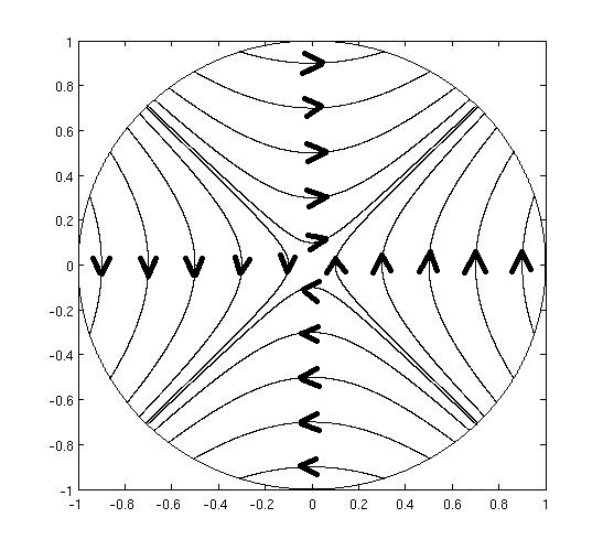
Figure 1: $\stackrel{{\scriptstyle\rightarrow}}{{j}}_{h}^{\left(1\right)}\left(1,0\right)$

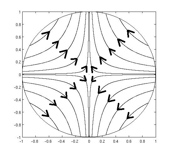
Figure 2: $\stackrel{{\scriptstyle\rightarrow}}{{j}}_{h}^{\left(1\right)}\left(i,0\right)$

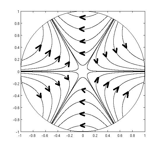
Figure 3: $\stackrel{{\scriptstyle\rightarrow}}{{j}}_{h}^{\left(2\right)}\left(1,0\right)$

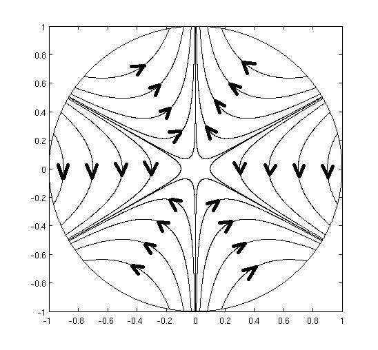
Figure 4: $\stackrel{{\scriptstyle\rightarrow}}{{j}}_{h}^{\left(2\right)}\left(i,0\right)$

In these Figures, as for all corresponding to this section, the arrows point out the direction of the electrical current flows. Just such nearest to the center are omitted by virtue of the space.

Let us focus our attention now onto the inhomogeneous case. Just as it happened before, the traces corresponding to the currents emerging from the formal powers $Z^{\left(0\right)}\left(1,0;\zeta\right)$ and $Z^{\left(0\right)}\left(i,0;\zeta\right)$ does not reach interesting diagrams.

$$\overrightarrow{j}^{\left(0\right)}\left(1,0;x_{1},x_{2}\right)=\left(\begin{array}[]{c}e^{2\sigma_{2}x_{2}+2\sigma_{3}x_{3}}\\ 0\\ 0\end{array}\right),\text{ }\overrightarrow{j}^{\left(0\right)}\left(i,0;x_{1},x_{2}\right)=\left(\begin{array}[]{c}0\\ e^{2\sigma_{1}x_{1}+2\sigma_{3}x_{3}}\\ 0\end{array}\right);$$ (54)

More illustrative examples arise when considering the current flows of $Z^{\left(1\right)}\left(1,0;\zeta\right)$ and $Z^{\left(1\right)}\left(i,0;\zeta\right)$ (for simplicity, next Figures are traced by fixing $x_{3}=0$):

$$\overrightarrow{j}^{\left(1\right)}\left(1,0;x_{1},x_{2}\right)=\left(\begin{array}[]{c}\frac{1}{\sigma_{2}}e^{\sigma_{2}x_{2}+2\sigma_{3}x_{3}}\sinh\left(\sigma_{2}x_{2}\right)\\ \frac{1}{\sigma_{1}}e^{\sigma_{1}x_{1}+2\sigma_{3}x_{3}}\sinh\left(\sigma_{1}x_{1}\right)\\ 0\end{array}\right),$$ (58)

$$\overrightarrow{j}^{\left(1\right)}\left(i,0;x_{1},x_{2}\right)=\left(\begin{array}[]{c}-\frac{1}{\sigma_{1}}e^{\sigma_{1}x_{1}+2\sigma_{2}x_{2}+2\sigma_{3}x_{3}}\sinh\left(\sigma_{1}x_{1}\right)\\ \frac{1}{\sigma_{2}}e^{2\sigma_{1}x_{1}+\sigma_{2}x_{2}+2\sigma_{3}x_{3}}\sinh\left(\sigma_{2}x_{2}\right)\\ 0\end{array}\right).$$ (62)

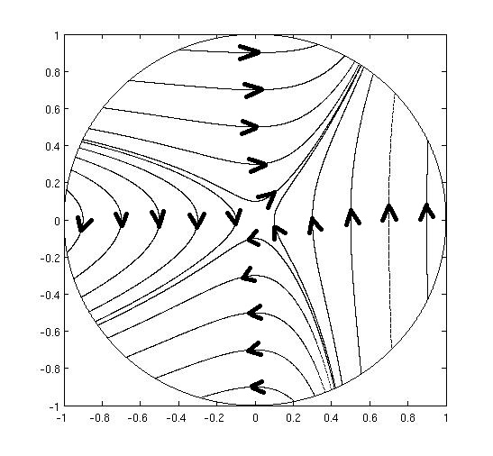
Figure 5: $\stackrel{{\scriptstyle\rightarrow}}{{j}}^{\left(1\right)}\left(1,0;x_{1},x_{2}\right)$

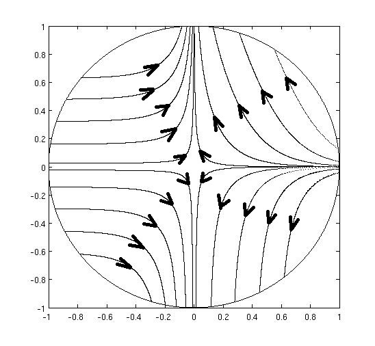
Figure 6: $\stackrel{{\scriptstyle\rightarrow}}{{j}}^{\left(1\right)}\left(i,0;x_{1},x_{2}\right)$

The diagrams are drawn considering $\sigma_{1}=3$ and $\sigma_{2}=1;$ and by evaluating the current density vectors $\overrightarrow{j}$ into a fixed point, displacing the mark in the direction of the vector in a distance of $0.01\%$ of the Cartesian norm in the subregions with higher conductivity, and $10\%$ in such with lower.

The Figures 7 and 8 show current patches when considering the remaining formal powers $\overrightarrow{j}^{\left(2\right)}\left(1,0;x_{1},x_{2}\right)$ and $\overrightarrow{j}^{\left(2\right)}\left(i,0;x_{1},x_{2}\right)$.

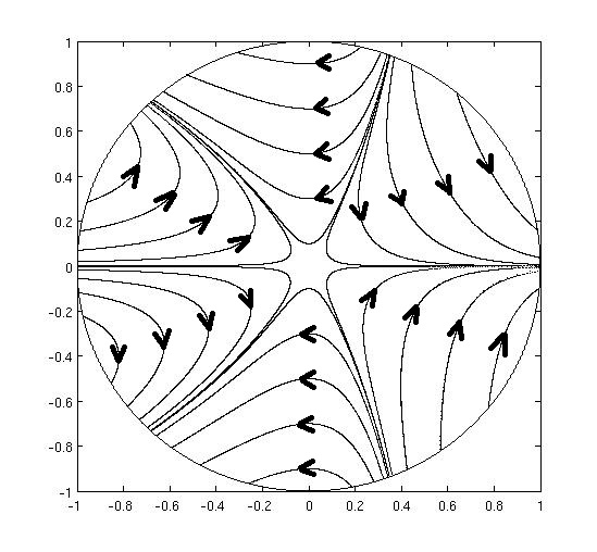
Figure 7: $\stackrel{{\scriptstyle\rightarrow}}{{j}}^{\left(2\right)}\left(1,0;x_{1},x_{2}\right)$

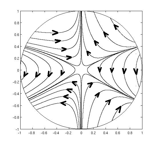
Figure 8: $\stackrel{{\scriptstyle\rightarrow}}{{j}}^{\left(2\right)}\left(i,0;x_{1},x_{2}\right)$

These short previews to the qualitative dynamics of the electrical current density vectors $\overrightarrow{j}^{\left(m\right)},~{}m=1,2;$ already allow us to point out some characteristics that seem to carry out useful patterns, when comparing them with the currents distributions for a constant conductivity function.

For instance, Figure 5 keeps the dynamical behavior of the traces found in Figure 1, presenting the most significant variations into the positive $x_{1}$-semiplane. Naturally, the magnitudes of the vector currents in both figures differ considerably when taking into account the conductivity values at every point into the domain $\Omega$. Still, a sort of dynamical relation might be suggested when adopting an appropriate point of view, as it will be posed in the next section, dedicated to the electric potentials at the boundary.

It is also remarkable that already watching the traces of the very first formal powers, we can infer that the most important disparities between the current patches corresponding to the homogeneous case and such of the inhomogeneous, will take place on the diagrams belonging to the lower formal degrees. This is, to such formal powers whose superindex are among the smallest.

This statement is based onto the location of what could be considered sink points and source points, following the terms employed in Complex Dynamical Systems (see e.g. [10]). Of course, in a strict sense, not any sink or source point is found inside the unitary circle, neither will be outside of it, because all traces behave asymptotically. Nevertheless, the reader could easily infer the location of such regions by watching the places around the perimeter where the patches seem to get closer to each other.

The bigger displacement of such regions takes place when appreciating the diagrams corresponding to the expressions with the smallest formal degrees. If the reader wishes to verify such behavior, perhaps standard computational languages for symbolic calculations can be useful in order to obtain in exact form some formal powers with higher degrees. Other case, it could be enough to trace again the posed diagrams considering, for example, $\sigma_{1}=\sigma_{2}=1$.

Thus, from this qualitative appreciation (at least for the inhomogeneous case just examined), we can observe a typical behavior of the formal powers when compared to the standard powers inside the unitary circle. We shall remember that this kind of behavior had been already remarked by L. Bers itself. Indeed, as it was mentioned before, professor Bers gave the complete proof for the case when $z\rightarrow z_{0}$ [2], opening the opportunity to study the behavior of the formal powers far away from their center.

3.3 The electric potential at the boundary

On the light of the last qualitative overview, a quantitative examination is in order. Let us pay our attention into one of the most important particular topics of the Generalized Ohm’s Law, when studied into bounded domains: The behavior of the electric potential $u$ at the boundary.

It is easy to see that for approaching the electric potentials $u^{\left(m\right)}(x_{1},x_{2})$ corresponding to the current density vectors posed before, numerical methods are already needed for the cases corresponding to the formal degree $2$. Let us consider by now some details of the electric potentials that can be obtained in exact form.

Ignoring the constant parts, the electric potential corresponding to the current $\overrightarrow{j}^{\left(0\right)}\left(1,0;x_{1},x_{2}\right)$ described in (54) is

$$u^{\left(0\right)}\left(1,0;x_{1},x_{2}\right)=\frac{1}{2\sigma_{1}}e^{-2\sigma_{1}x_{1}},$$

whereas the one for $\overrightarrow{j}^{\left(0\right)}\left(i,0;x_{1},x_{2}\right)$ is

$$u^{\left(0\right)}\left(i,0;x_{1},x_{2}\right)=\frac{1}{2\sigma_{2}}e^{-2\sigma_{2}x_{2}}.$$

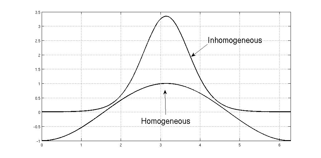
Figure 9: $u^{\left(0\right)}\left(1,0;x_{1},x_{2}\right)$

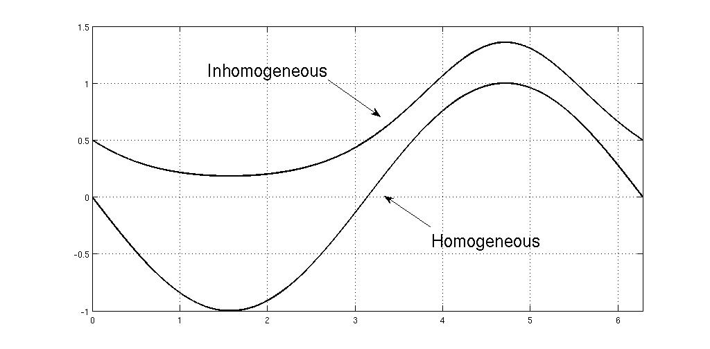
Figure 10: $u^{\left(0\right)}\left(i,0;x_{1},x_{2}\right)$

As it is pointed out, the graphics included in Figure 9 correspond to the electric potential of the inhomogeneous case, titling the Figure with the abbreviated notation $u^{\left(0\right)}\left(1,0\right),$ and of the homogeneous case denoted by $u_{h}^{\left(0\right)}\left(1,0\right)$. The graphics are traced by simply considering the value of the potentials at the boundary. This is, $x_{1}=\cos\theta$ and $x_{2}=\sin\theta;$ $\theta\in[0,2\pi].$ The same is done for the next Figure, where the graphics for $u^{\left(0\right)}\left(i,0\right)$ and $u_{h}^{\left(0\right)}\left(i,0\right)$ are presented.

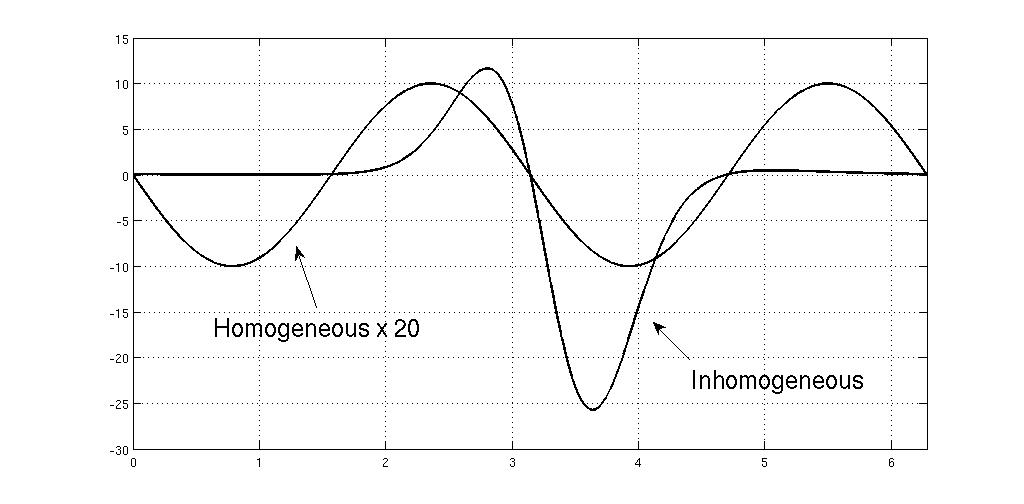
Figure 11: $u^{\left(1\right)}\left(1,0;x_{1},x_{2}\right)$

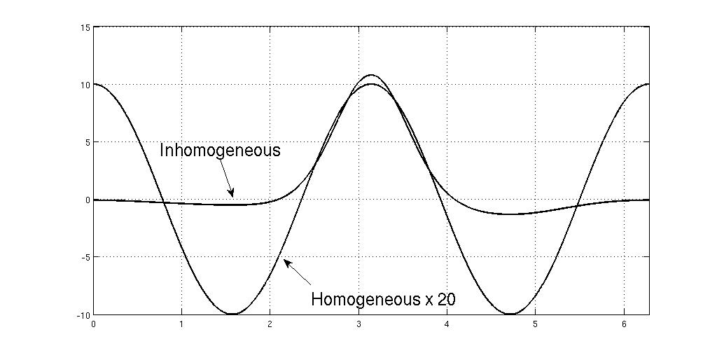
Figure 12: $u^{\left(1\right)}\left(i,0;x_{1},x_{2}\right)$

Again, as it was already expected, from a certain point of view it could be possible to assert that there exist a pattern on the dynamical behavior of these potentials at the boundary. For these cases, as the following graphics could suggest, the boundary potentials corresponding to the lower formal degrees, seem to hold the closest dynamical behavior.

For the current vectors $\overrightarrow{j}^{\left(1\right)}\left(1,0;x_{1},x_{2}\right)$ and $\overrightarrow{j}^{\left(1\right)}\left(i,0;x_{1},x_{2}\right)$ of (58), the electric potentials are

$$u^{\left(1\right)}\left(1,0;x_{1},x_{2}\right)=\frac{1}{4\sigma_{1}\sigma_{2}}\left(e^{-2\sigma_{1}x_{1}}+e^{-2\sigma_{2}x_{2}}-e^{-2\sigma_{1}x_{1}-2\sigma_{2}x_{2}}\right),$$

$$u^{\left(1\right)}\left(i,0;x_{1},x_{2}\right)=\frac{x_{1}}{2\sigma_{1}}-\frac{x_{2}}{2\sigma_{2}}+\frac{1}{4\sigma_{1}^{2}}e^{-2\sigma_{1}x_{1}}-\frac{1}{4\sigma_{2}^{2}}e^{-2\sigma_{2}x_{2}}.$$

The behaviors of the potentials illustrated in Figure 11 and Figure 12, could still suggest the existence of some dynamical relation, pointing out that it was already necessary to scale the graphics corresponding to the homogeneous case by a factor of $20,$ in order to show them together with such corresponding to the inhomogeneous case.

Other hand, the dynamics performed in this examples can be located nearer of the behaviors expected when analyzing the electric potentials from a classical point of view: The variations of the potentials at the boundary does not hold any simple relation with the variations of the conductivity inside the domain $\Omega$. Still, by these basic examples, it is possible to suggest that perhaps from the point of view of the Pseudoanalytic Function Theory, applied to the study of the Generalized Ohm’s Law, the instability of the electric potential at the boundary, when changes of the conductivity function inside the domain are taking place, could be diminished if the changes are considered for every formal electric potential individually.

This could well represent an important contribution for better understanding inverse problems, as it is the one posed by A. P. Calderon in 1980 [3], known in medical imaging as Electrical Impedance Tomography.

4 A technique for approaching separable-variables conductivity functions

A very important problem is located around how to approach a separable-variable conductivity function once it is given a finite set of points inside a domain $\Omega$ in the plane, where the electric conductivity is known (a very natural starting point for many physical examinations).

This is a critical matter, since all procedures posed in this work are based upon the idea of possessing an explicit separable-variables conductivity function. Indeed, it is very difficult to find among the literature any reference about specific methods for interpolating separable-variables functions, even for the two-dimensional case. Perhaps the following idea could serve as a temporally departure point.

Let us suppose we have a finite set of $k_{1}+1$ parallel lines to the $x_{1}$-axe, dividing the domain $\Omega$ into $k_{1}$ segments. Suppose we also have a set of $k_{2}+1$ lines parallel to the $x_{2}$-axe, dividing again the segments obtained from the first step. The result will be a sort of grill, with a finite number $k<k_{1}\times k_{1}$ of intersections within the domain $\Omega$, hence we can introduce a set of points $z_{k}=(z_{k}^{\prime},z_{k}^{\prime\prime})$ located precisely at every intersection inside $\Omega$, where $z_{k}^{\prime}$ represents the $x_{1}$-coordinate of $z_{k}$ and $z_{k}^{\prime\prime}$ is the $x_{2}$-coordinate. Finally, let us assign a conductivity value $\sigma\left(z_{k}\right)$ to each point $z_{k}.$

Starting with the segment of line intersecting the $x_{2}$-axe at the maximum value reached inside $\Omega$, we can interpolate all values $\sigma\left(z_{k}\right)$ corresponding to the points $z_{k}$ contained within that line. Hence we can pose a continuos function of the form

$$\alpha_{1}\left(x_{1}\right)=\frac{f_{1}\left(x_{1}\right)}{z_{1}^{\prime\prime}+K},$$

where $z_{1}^{\prime\prime}$ is the common $x_{2}$-coordinate of all points $z_{k}$ belonging to the line segment on which the interpolating function $f_{1}$ is defined, and $K$ is an arbitrary real constant such that $x_{2}+K\neq 0,$ $x_{2}\in\Omega.$

The same can be done for the rest of line segments parallel to $x_{1}$ found into $\Omega.$

We can then define the following piecewise function $\sigma\left(x_{1},x_{2}\right):$

$$\sigma\left(x_{1},x_{2}\right)=\left\{\begin{array}[]{l}\left(x_{2}+K\right)\alpha_{1}\left(x_{1}\right):x_{2}\in\left[\max x_{2}:x_{2}\in\Omega,z_{1}^{\prime\prime}-\frac{z_{1}^{\prime\prime}+z_{2}^{\prime\prime}}{2}\right);\\ \left(x_{2}+K\right)\alpha_{2}\left(x_{1}\right):x_{2}\in\left[z_{1}^{\prime\prime}-\frac{z_{1}^{\prime\prime}+z_{2}^{\prime\prime}}{2},z_{2}^{\prime\prime}-\frac{z_{2}^{\prime\prime}+z_{3}^{\prime\prime}}{2}\right);\\ \left(x_{2}+K\right)\alpha_{3}\left(x_{1}\right):x_{2}\in\left[z_{2}^{\prime\prime}-\frac{z_{2}^{\prime\prime}+z_{3}^{\prime\prime}}{2},z_{3}^{\prime\prime}-\frac{k_{3}^{\prime\prime}+k_{4}^{\prime\prime}}{2}\right);\\ \lx@intercol\hfil...\hfil\lx@intercol\\ \left(x_{2}+K\right)\alpha_{k_{1}}\left(x_{1}\right):x_{2}\in\left[z_{k_{1}-1}^{\prime\prime}-\frac{z_{k_{1}-1}^{\prime\prime}+z_{k_{1}}^{\prime\prime}}{2},\min x_{2}:x_{2}\in\Omega\right];\end{array}\right.$$

where $z_{k}^{{}^{\prime\prime}}:k=1,2,...,k_{1}$ are the common $x_{2}$-coordinates of every set of $z_{k}$ points belonging to the same line segment parallel to $x_{1}$ inside $\Omega$.

It is easy to see that the piecewise function $\sigma\left(x_{1},x_{2}\right)$ defined in the last expression is a separable-variable function, so it can be employed when numerical calculations are performed for approaching higher formal powers than those considered in this work. Notice also that the same idea can be extended for segmentations of a bounded domain $\Omega$ by means of polar traces.

Moreover, this basic idea could be also useful when considering the resulting electrical impedance equation when studying the monochromatic time-dependet case:

$$\text{div}\left(\gamma\text{grad}u\right)=0.$$

Here $\gamma=i\omega\varepsilon+\sigma$ represents the electrical impedance, $\omega$ is the wave frequency and $\varepsilon$ is a scalar function denoting the electrical permittivity. The reader can verify that virtually all mathematical methods explained in the above paragraphs can be extended for this complex case.

Acknowledgement 1

The author would like to acknowledge the support of CONACyT project 106722, Mexico.

References

• [1] K. Astala and L. Päivärinta, Calderón’s inverse conductivity problem in plane, Annals of Mathematics No. 163, 265-299, 2006.
• [2] L. Bers, Theory of Pseudo-Analytic Functions, Institute of Mathematics and Mechanics, New York University, New York, 1953.
• [3] A. P. Calderon, On an inverse boundary value problem, Seminar on Numerical Analysis and its Applications to Continuum Physics, Sociedade Brasileira de Matematica, pp. 65-73, 1980.
• [4] R. Castillo P., V. V. Kravchenko, R. Resendiz V., Solution of boundary value and eigenvalue problems for second order elliptic operators in the plane using pseudoanalytic formal powers, Mathematical Methods in the Applied Sciences, Available in electronic format in arXiv:1002.1110v1 [math.AP], 2010.
• [5] E. Demidenko, Separable Laplace equation, magic Toeplitz matrix, and generalized Ohm’s law, Applied Mathematics and Computation, Vol. 181, Issue 2, 1313-1327, Elsevier, 2006.
• [6] V. V. Kravchenko, Applied Pseudoanalytic Function Theory, Series: Frontiers in Mathematics, ISBN: 978-3-0346-0003-3, 2009.
• [7] V. V. Kravchenko, Applied Quaternionic Analysis, Researches and Exposition in Mathematics, Vol. 28, Heldermann Verlag, 2003.
• [8] V. V. Kravchenko, H. Oviedo, On explicitly solvable Vekua equations and explicit solution of the stationary Schrödinger equation and of the equation $\text{div}\left(\sigma\nabla u\right)=0$, Complex Variables and Elliptic Equations, Vol. 52, No. 5, pp. 353-366, 2007.
• [9] V. V. Kravchenko, M. P. Ramirez T., On Bers generating functions for first order systems of mathematical physics, Advances in Applied Clifford Algebras ISSN 0188-7009 (Accepted for publication). Available in electronic in arXiv:1001.0552v1, 2010.
• [10] H. Peitgen, H. Jürgens, D. Saupe, Chaos and Fractals: New Frontiers of Science, Springer-Verlag, 1993.
• [11] G. N. Polozhy, Generalization of the theory of analytic functions of complex variables: p-analytic and (p,q)-analytic functions and some applications, Kiev University Publishers (in Russian), 1965.
• [12] M. P. Ramirez T., J. J. Gutierrez C., V. D. Sanchez N. and E. Bernal F., New Solutions for the Three-Dimensional Electrical Impedance Equation and its Application to the Electrical Impedance Tomography Theory, Proceedings of the WCE 2010, Vol. 1, pp. 527-532, U.K., 2010.
• [13] M. P. Ramirez T., V. D. Sanchez N., O. Rodriguez T. and A. Gutierrez S., On the General Solution for the Two-Dimensional Electrical Impedance Equation in Terms of Taylor Series in Formal Powers, IAENG International Journal of Applied Mathematics, 39:4, 2009.
• [14] M. P. Ramirez T., O. Rodriguez T., J. J. Gutierrez C., New Exact Solutions for the Three-Dimensional Electrical Impedance Equation applying Quaternionic Analysis and Pseudoanalytic Function Theory, Proceedings of CCE 2009, IEEE, pp. 344-349, 2009.
• [15] I. N. Vekua, Generalized Analytic Functions, International Series of Monographs on Pure and Applied Mathematics, Pergamon Press, 1962.