Spectral properties of quarks above $T_{c}$ – thermal mass, dispersion relation, and self-energy –

Abstract:

Spectral properties of quarks above the critical temperature for deconfinement are analyzed in quenched lattice QCD on lattices of size $128^{3}\times 16$. We study quark spectral function in energy and momentum space, focusing on the values of the thermal mass and the dispersion relations of normal and plasmino modes at nonzero momentum, as well as their spatial volume dependence. Our numerical result suggests that the dispersion relation of the plasmino mode has a minimum at nonzero momentum even near the critical temperature. The quark self-energy is also analyzed by using the analyticy of the inverse propagator, which is found to be consistent with the spectral function estimated by the two-pole ansatz.

1 Introduction

At asymptotically high temperature ($T$), properties of strongly interacting matter described by Quantum Chromodynamics (QCD) can be calculated using perturbative techniques. In this limit, it is known that the collective excitations of quarks develop a mass gap (thermal mass) and a decay rate proportional to $gT$ and $g^{2}T$, respectively, where $g$ denotes the gauge coupling [1]. Furthermore, the dispersion relation splits into two branches, the normal and plasmino modes. As the decay rate parametrically grows faster than the thermal mass as $g$ increases, it is naïvely expected that the quark quasi-particles cease to exist as $T$ is lowered. On the other hand, quark number scaling of the elliptic flow observed in RHIC experiments indicates the existence of quasi-particles having a quark quantum number [2]. To understand properties of the matter near $T_{c}$, especially the quasi-particle nature of elementary excitations, therefore, it is desirable to explore the spectral properties of quarks within nonperturbative techniques.

Recently, the correlation function of quarks at nonzero $T$ has been analyzed on the quenched lattice with size up to $N_{\sigma}^{3}\times N_{\tau}=64^{3}\times 16$ in Landau gauge [3]. In these studies, it is found that the quark correlation function above $T_{c}$ obtained on the lattice is well reproduced by the two-pole ansatz for the spectral function, where the two poles correspond to the normal and plasmino modes. In the chiral limit these modes have identical quasi-particle masses, which are identified to be the thermal mass, that are approximately proportional to $T$. These calculations, however, also showed that the quasi-particle masses, which perturbatively arise through the resummation of infra-red sensitive loops [1], are strongly dependent on the physical volume, $V$, used in the lattice calculations.

The purpose of the present study is to extend the analysis in Refs. [3] to much larger spatial volume, $N_{\sigma}^{3}\times N_{\tau}=128^{3}\times 16$ [4]. This analysis enables us to investigate the spatial volume dependence in more detail. The large spatial volume also allows to directly analyze the momentum dependence of excitation spectra, i.e. the dispersion relations, more precisely. To obtain better understanding on the spectral property of quarks, in addition to the analysis of the spectral function, we also try to examine the quark self-energy by numerically taking the inverse of the quark propagator.

2 Quark spectral function and fitting ansatz

Excitation properties of the quark field are encoded in the quark spectral function $\rho_{\mu\nu}(\omega,\vec{p})$, with $\mu$ and $\nu$ denoting Dirac indices. The Dirac structure of $\rho_{\mu\nu}(\omega,\vec{p})$ at finite temperature is decomposed as

$$\rho_{\mu\nu}(\omega,\vec{p})=\rho_{0}(\omega,p)(\gamma^{0})_{\mu\nu}-\rho_{\rm v}(\omega,p)(\hat{\vec{p}}\cdot\vec{\gamma})_{\mu\nu}+\rho_{\rm s}(\omega,p)1_{\mu\nu},$$ (1)

where $p=|\vec{p}|$ and $\hat{\vec{p}}=\vec{p}/p$. In the present study we consider the spectral function above $T_{c}$ for two cases; (1) at zero momentum, and (2) in the chiral limit. In these cases, the Dirac structure of $\rho_{\mu\nu}(\omega,\vec{p})$ are decomposed by using projection operators [3]. With $p=0$, $\rho_{\rm v}(\omega,p)$ vanishes in Eq. (1) and $\rho_{\mu\nu}(\omega,\vec{p}=\vec{0})$ is decomposed with the projection operators $L_{\pm}=(1\pm\gamma^{0})/2$ as

$$\rho(\omega,\vec{0})=\rho^{\rm M}_{+}(\omega)L_{+}\gamma^{0}+\rho^{\rm M}_{-}(\omega)L_{-}\gamma^{0}.$$ (2)

In the chiral limit and for $T>T_{c}$, the system possesses the chiral symmetry and $\rho_{\rm s}(\omega,p)$ vanishes. In this case, $\rho_{\mu\nu}(\omega,\vec{p})$ is decomposed with the projection operators $P_{\pm}(\vec{p})=(1\pm\gamma^{0}\hat{\vec{p}}\cdot\vec{\gamma})/2$ as

$$\rho(\omega,\vec{p})=\rho^{\rm P}_{+}(\omega,p)P_{+}(\vec{p})\gamma^{0}+\rho^{\rm P}_{-}(\omega,p)P_{-}(\vec{p})\gamma^{0}.$$ (3)

In order to extract $\rho_{\mu\nu}(\omega,\vec{p})$ from lattice QCD simulations we have analyzed the quark correlation function in Euclidean space

$$S_{\mu\nu}(\tau,\vec{p})=\frac{1}{V}\int d^{3}xd^{3}y\mbox{e}^{i{\bf p}\cdot({\bf x}-{\bf y})}\langle\psi_{\mu}(\tau,\vec{x})\bar{\psi}_{\nu}(0,\vec{y})\rangle,$$ (4)

on the lattice in quenched approximation in Landau gauge. Nonperturbatively-improved clover fermion is used for the analysis. Equation (4) is related to the spectral function as

$$S_{\mu\nu}(\tau,\vec{p})=\int_{-\infty}^{\infty}d\omega\frac{\mbox{e}^{(1/2-\tau T)\omega/T}}{\mbox{e}^{\omega/2T}+\mbox{e}^{-\omega/2T}}\rho_{\mu\nu}(\omega,\vec{p}).$$ (5)

In order to examine the quark spectral function from lattice correlator, we follow the approach taken in [3], which makes use of a two-pole ansatz for the spectrum,

$$\rho^{\rm M,P}_{+}(\omega)=Z_{1}\delta(\omega-E_{1})+Z_{2}\delta(\omega+E_{2}).$$ (6)

Here, $Z_{1,2}$, and $E_{1,2}>0$, are fitting parameters that will be determined from correlated fits to the lattice correlator: $Z_{1,2}$ and $E_{1,2}$ represent the residues and positions of poles, respectively. When comparing the fit results with spectral functions obtained in perturbative calculations one can identify the pole at $\omega=E_{1}$ to be the normal mode, while the one at $\omega=-E_{2}$ corresponds to the plasmino mode [5, 6]. To determine the fit parameters with correlated fits, we use lattice data points at $\tau_{\rm min}\leq\tau/a\leq N_{\tau}-\tau_{\rm min}$ with $\tau_{\rm min}=4$. We found that the ansatz Eq. (6) gives a reasonable chi-square, $\chi^{2}/{\rm dof}\simeq 1$, over wide parameter ranges [3]; see, however, Ref. [4] which discusses problems associated with the analysis of the spectral function with an ansatz.

3 Thermal mass and dispersion relations

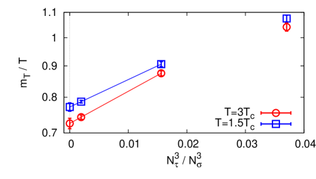
Figure 1: Extrapolation of the thermal mass of the quark $m_{T}$ obtained by the pole ansatz to the infinite volume limit for $T/T_{c}=3$, $1.5$.

The quark spectral function is analyzed (1) for $p=0$ as a fuctions of bare quark mass, $m_{0}$, and (2) for $m_{0}=0$ as a fuctions of $p$. For each case, we use the projection Eqs. (2) and (3), respectively.

In the analysis of $\rho^{\rm M}_{\pm}(\omega)$ at $p=0$ on the largest lattice with $N_{\sigma}/N_{\tau}=8$, we found that the $m_{0}$ dependence of fitting parameters qualitatively agrees with previous results obtained on lattices with $N_{\sigma}/N_{\tau}=4$ and $3$ in Ref. [3]. From the $m_{0}$ dependence of $\rho^{\rm M}_{\pm}(\omega)$ one can define the critical hopping parameter for the chiral limit and the thermal mass, $m_{T}$ [3, 4]. In Fig. 1, we show the value of $m_{T}$ with $N_{\sigma}/N_{\tau}=8$, $4$ and $3$ for $T/T_{c}=1.5$ and $3$. To infer the thermal mass in the infinite volume limit, we performed an extrapolation of $m_{T}$ to infinite volume with an ansatz $m_{T}(1/V)\sim m_{T}(0)\exp(c/V)$ using the results with $N_{\sigma}/N_{\tau}=8$ and $4$. The result of this extrapolation is shown in Fig. 1. Within the extrapolation, the value of $m_{T}(1/V\to 0)$ coincides the one obtained with $N_{\sigma}/N_{\tau}=8$ within the statistical error.

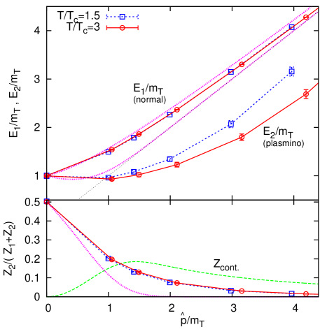
Figure 2: Dependences of the fitting parameters $E_{1}$ and $E_{2}$ and the ratio $Z_{2}/(Z_{1}+Z_{2})$ on the lattice momentum $\hat{p}=(1/a)\sin(pa)$ for $T/T_{c}=1.5$ and $3$. See, the text for the explanation of other lines.

Next, we set $m_{0}=0$ and analyze the momentum dependence of the excitation spectra at nonzero momentum using the decomposition given in Eq. (3). In Fig. 2 we show the momentum dependence of $E_{1}$ and $E_{2}$ normalized by $m_{T}$ and $Z_{2}/(Z_{1}+Z_{2})$ for $T/T_{c}=1.5$ and $3$. The horizontal axis represents the momentum of free Wilson fermions on the lattice, $\hat{p}=(1/a)\sin pa$, normalized by $m_{T}$. The figure shows that $E_{1}>E_{2}$ is satisfied in accordance with the relation between the normal and plasmino dispersions at asymptotically high temperature. The figure also shows that the value of $E_{2}$ for the lowest non-zero momentum, $p_{\rm min}=2\pi(N_{\tau}/N_{\sigma})T$, is significantly lower than $m_{T}$. Provided that the value of $E_{2}$ in our two-pole ansatz represents the dispersion relation of the plasmino mode, this result serves as direct evidence for the existence of the plasmino minimum in the non-perturbative analysis. One, however, has to be careful with this interpretation because the Euclidean correlator is insensitive to the spectral function at low energy, $|\omega|\lesssim T$, and analysis of the spectrum in this energy range has large uncertainty [4].

4 Quark self-energy

In order to investigate dynamical properties of the system in lattice simulations, one has to take the analytic continuation from a Euclidean correlation function obtained on the lattice to a real-time propagator. This analytic continuation, however, is a famous ill-posed problem, because one has to infer the real-time propagator, which is a continuous function, from finite and noisy data obtained on the Monte Carlo simulations. In previous sections, we have used an ansatz Eq. (5) for the spectral function to avoid this difficulty. Although such an analysis would be convenient to understand a qualitative structure of the spectrum, details of the spectrum is not accessible. Even if one uses the maximum entropy analysis which infers the spectral function without introducing an ansatz, the resulting spectral image has uncertainty in the analyses of lattice correlators with typical statistics. To make the analytic continuation more robust, therefore, it is desirable to have a different formula which relates real- and imaginary-time functions besides Eq. (5).

Here, we propose to exploit the inverse propagator for this purpose. The inverse of the retarded quark propagator, $S^{R}(\omega,p)$, is written as

$$\left[S^{R}(\omega,p)\right]^{-1}=\left[S^{R}_{0}(\omega,p)\right]^{-1}-\Sigma^{R}(\omega,p),$$ (7)

where $S^{R}_{0}(\omega,p)$ and $\Sigma^{R}(\omega,p)$ denote the retarded free-quark propagator and self-energy, respectively. Let us first derive a formula like Eq. (5) relating $[S^{R}(\omega,p)]^{-1}$ to a Euclidean function. For this purpose we first remark that $[S^{R}(\omega,p)]^{-1}$ is analytic in the upper-half complex-energy plane, $\mathbb{C}^{+}$, as well as $S^{R}(\omega,p)$. This statement is easily verified by the fact that $\Sigma^{R}(\omega,p)$ is analytic in $\mathbb{C}^{+}$ by definition. Using this property of $[S^{R}(\omega,p)]^{-1}$ and Kramers-Kronig relation, by taking a similar procedure to derive Eq. (5) one arrives at a formula which connects the inverse retarded propagator to a Euclidean function

$$\left[\tilde{S}\right]^{-1}(\tau,p)=\int_{-\infty}^{\infty}d\omega\frac{\mbox{e}^{(1/2-\tau T)\omega/T}}{\mbox{e}^{\omega/2T}+\mbox{e}^{-\omega/2T}}\mbox{Im}\left[S^{R}(\omega,p)\right]^{-1}=-\int_{-\infty}^{\infty}d\omega\frac{\mbox{e}^{(1/2-\tau T)\omega/T}}{\mbox{e}^{\omega/2T}+\mbox{e}^{-\omega/2T}}\mbox{Im}\Sigma^{R}(\omega,p),$$ (8)

where $[\tilde{S}]^{-1}(\tau,p)$ is the inverse of the Matsubara propagator $\tilde{S}(\tau,p)$. Remark, however, that Eq. (8) cannot apply to $\tau=0$. In the last equality of Eq. (8) we have used the fact that $[S_{0}(\omega,p)]^{-1}$ is real, and hence $\mbox{Im}[S(\omega,p)]^{-1}=-\mbox{Im}\Sigma^{R}(\omega,p)$.

The inverse propagator $[\tilde{S}]^{-1}(\tau,p)$ is calculated by inverting the correlation function $\tilde{S}(\tau,p)$ obtained on the lattice. Since $\tilde{S}(\tau,p)$ is block-diagonal in frequency space, this inversion is most conveniently taken after the Fourier transformation, i.e.

$$\left[\tilde{S}\right]^{-1}(\tau,p)=T\sum_{n}\left[\tilde{S}(i\omega_{n},p)\right]^{-1}e^{-i\tau\omega_{n}},$$ (9)

with Matsubara frequency $\omega_{n}=(2n+1)\pi T$, where $[~{}~{}]^{-1}$ in the r.h.s. represents an inverse of $4\times 4$ matrix for Dirac indices, while that in the l.h.s. means the inverse of the whole propagator. Since Eq. (8) has the same form as Eq. (5), once $[S]^{-1}(\tau,p)$ is constructed one can infer the real-time self-enegy $\mbox{Im}\Sigma(\omega,p)$ with the same techniques to analyze the spectral function with Eq. (5), such as the maximum entropy method.

Remarks in constructing $[\tilde{S}]^{-1}(\tau,p)$ are in order here. First, $[\tilde{S}]^{-1}(\tau,p)$ is not the thermal average of the fermion matrix $K=iD/-m$. This is because the propagator in the l.h.s. of Eq. (7) is defined by the thermal average of $K^{-1}$. The thermal average thus must be taken for the inverse of $K$. Second, to obtain $[\tilde{S}]^{-1}(\tau,p)$ one needs all elements of $\tilde{S}(\tau,p)$ including the value at $\tau=0$. For correlators having a positive mass dimension, $\tilde{S}(\tau,p)$ is singular at $\tau=0$ in the continuum limit, and one must exclude this point from the analysis. The quark correlator, on the other hand, has zero mass dimension and takes a finite value even at the origin. No difficulty thus in principle arises with the use of this point. The use of $\tilde{S}(\tau,p)$ near the source, however, is troublesome because correlators with small $\tau/a$ receive strong lattice artifacts due to the overlap of operators on the lattice. We will later investigate this effect by directly analysing $[\tilde{S}]^{-1}(\tau,p)$.

The analysis of $[\tilde{S}]^{-1}(\tau,p)$ and ${\rm Im}\Sigma^{R}(\omega,p)$ has more advantages. First, in the perturbative analysis of quark propagator one must first calculate the self-energy. In this sense, the self-energy is more useful and fundamental quantity than the propagator in the analytic studies. If one wants to compare the analytic result with the lattice one, the comparison is usually made in terms of the propagator. The data of the inverse propagator, $[\tilde{S}]^{-1}(\tau,p)$, on the other hand, enables to make this comparison in terms of the self-energy. Next, microscopic physics behind the spectral properties would become more apparent through the analysis of $\mbox{Im}\Sigma(\omega,p)$. Because the value of $\mbox{Im}\Sigma(\omega,p)$ is related to elementary processes via the optical theorem, one can give a direct interpretations to the structure of $\mbox{Im}\Sigma(\omega,p)$. Of course, $\rho(\omega,p)$ and $\mbox{Im}\Sigma(\omega,p)$ should have one-to-one correspondence under a given regularization, and in principle one of these functions must contain all information of excitation properties. In lattice simulations, however, one cannot determine the real-time function definitely. The analysis of a different function thus can make different physics more apparent.

Because the same correlator as in Eq. (5) is used in the construction of $[\tilde{S}]^{-1}(\tau,p)$, one may think that Eq. (8) does not provide any new information on the real-time function besides Eq. (5). We, however, remark that Eq. (8) encodes the analyticy of the inverse propagator in $\mathbb{C}^{+}$, which is not taken into account in Eq. (5). An appropriate use of Eq. (8) thus should enable us to extract additional information on the real-time function.

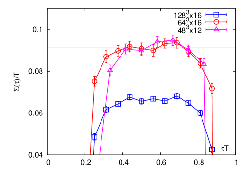
Figure 3: The quark self-energy in Euclidean space as a function of imaginary time $\tau$ for $T/T_{c}=3$.

In Fig. 3, we show the inverse quark propagator $[\tilde{S}]^{-1}_{0}(\tau,0)={\rm Tr}[[\tilde{S}]^{-1}(\tau,0)\gamma^{0}]$ in imaginary time in the chiral limit for $T=3T_{c}$, with several values of $N_{\sigma}$ and $N_{\tau}$, which are constructed from the same quark correlators analyzed in the previous sections [3, 4]. Errorbars are estimated by the jackknife analysis. In the figure, we also show the values of $[\tilde{S}]^{-1}_{0}(\tau,0)$ corresponding to the spectral function estimated by the two-pole ansatz Eq. (6) by the thin-solid lines: The spectrum in the chiral limit, $\rho(\omega,0)=Z(\delta(\omega-m_{T})+\delta(\omega+m_{T}))$, corresponds to ${\rm Im}[S(\omega,0)]^{-1}_{0}={\rm Im}{\rm Tr}[\Sigma(\omega,0)\gamma^{0}]=m_{T}^{2}/(TZ)\delta(\omega)$. One finds from the figure that $[S]^{-1}_{0}(\tau,0)$ is consistent with the prediction of the two-pole ansatz within statistics near $\tau T=0.5$. On the other hand, $[\tilde{S}]^{-1}_{0}(\tau,0)$ shows a strong deviation from the constant near the source. Similar results are obtained for nonzero $m_{0}$ and $p$.

The fact that the values of $[\tilde{S}]^{-1}_{0}(\tau,p)$ coincide with the ones predicted by the pole ansatz around $\tau T=0.5$ would support (1) the validity of the pole ansatz for the quark spectrum, and (2) the relevance of the evaluation of ${\rm Im}\Sigma(\omega,p)$ with Eq. (8). The large deviation from the constant near the source would be attributed to the distortion effects; in fact, the deviation is more prominent on the course lattice. The errorbars and the distortion effect with the present lattice data are too large to constrain the form of the spectral function with Eq. (8). Much finer lattice and higher statistics are needed to proceed the analysis of the self-energy with Eq. (8) further.

To summarize, in this report we analyzed the spectral properties of quarks on the quenched lattice with size $N_{\sigma}^{3}\times N_{\tau}=128^{3}\times 16$. We found that the spatial volume dependence of the quark thermal mass defined by the pole ansatz tends to converge on this volume. The dispersion relations of the normal and plasmino modes are investigated within the two-pole ansatz. The result indicates the existence of a minimum of the plasmino dispersion at nonzero momentum. We also introduced attempts to analyze the quark self-energy.

This proceedings is based on the collabolation done with O. Kaczmarek, F. Karsch, W. Soeldner, M. Asakawa, and S. Takotani. Numerical simulations of this study have been performed on the BlueGene/L at the New York Center for Computational Sciences (NYCCS).

References

- [1] M. Le Bellac, Thermal Field Theory (Cambridge University Press, Cambridge, England 1996).
- [2] R. J. Fries, B. Muller, C. Nonaka and S. A. Bass, Phys. Rev. C 68, 044902 (2003) [arXiv:nucl-th/0306027].
- [3] F. Karsch and M. Kitazawa, Phys. Lett. B 658, 45 (2007) [arXiv:0708.0299 [hep-lat]]; Phys. Rev. D 80, 056001 (2009) [arXiv:0906.3941 [hep-lat]].
- [4] O. Kaczmarek, F. Karsch, M. Kitazawa, and W. Soeldner, in preparation.
- [5] G. Baym, J. P. Blaizot and B. Svetitsky, Phys. Rev. D 46, 4043 (1992).
- [6] M. Kitazawa, T. Kunihiro and Y. Nemoto, Phys. Lett. B 633, 269 (2006) [arXiv:hep-ph/0510167]; Prog. Theor. Phys. 117, 103 (2007) [arXiv:hep-ph/0609164]; M. Kitazawa, T. Kunihiro, K. Mitsutani and Y. Nemoto, Phys. Rev. D 77, 045034 (2008) [arXiv:0710.5809 [hep-ph]].