Persistent Magnetic Wreaths in a Rapidly Rotating Sun

Abstract

When our Sun was young it rotated much more rapidly than now. Observations of young, rapidly rotating stars indicate that many possess substantial magnetic activity and strong axisymmetric magnetic fields. We conduct simulations of dynamo action in rapidly rotating suns with the 3-D MHD anelastic spherical harmonic (ASH) code to explore the complex coupling between rotation, convection and magnetism. Here we study dynamo action realized in the bulk of the convection zone for a system rotating at three times the current solar rotation rate. We find that substantial organized global-scale magnetic fields are achieved by dynamo action in this system. Striking wreaths of magnetism are built in the midst of the convection zone, coexisting with the turbulent convection. This is a surprise, for it has been widely believed that such magnetic structures should be disrupted by magnetic buoyancy or turbulent pumping. Thus, many solar dynamo theories have suggested that a tachocline of penetration and shear at the base of the convection zone is a crucial ingredient for organized dynamo action, whereas these simulations do not include such tachoclines. We examine how these persistent magnetic wreaths are maintained by dynamo processes and explore whether a classical mean-field $\alpha$-effect explains the regeneration of poloidal field. We find that the global-scale toroidal magnetic fields are maintained by an $\Omega$-effect arising from the differential rotation, while the global-scale poloidal fields arise from turbulent correlations between the convective flows and magnetic fields. These correlations are not well represented by an $\alpha$-effect that is based on the kinetic and magnetic helicities.

Feb 11, 2010

1. Stellar Magnetism and Rotation

Most stars are born rotating quite rapidly. They can arrive on the main sequence with rotational velocities as high as 200 $\mathrm{km}\>\mathrm{s}^{-1}$ (Bouvier et al. 1997). Stars with convection zones at their surfaces, like the Sun, slowly spin down as they shed angular momentum through their magnetized stellar winds (e.g., Weber & Davis 1967; Skumanich 1972; MacGregor & Brenner 1991). The time needed for significant spindown appears to be a strong function of stellar mass (e.g., Barnes 2003; West et al. 2004): solar-mass stars slow less rapidly than somewhat less massive G and K-type stars, but still appear to lose much of their angular momentum by the time they are as old as the Sun. Present day observations of the solar wind likewise indicate that the current angular momentum flux from the Sun is a few times 10³⁰ dyn cm (e.g., Pizzo et al. 1983), suggesting a time scale for substantial angular momentum loss of a few billion years. Thus the Sun likely rotated significantly more rapidly in its youth than it does today.

1.1. Rotation-Activity Relations

Rotation appears to be inextricably linked to stellar magnetic activity. Observations indicate that in stars with extensive convective envelopes, chromospheric and coronal activity – which partly trace magnetic heating of stellar atmospheres – first rise with increasing rotation rate, then eventually level off at a constant value for rotation rates above a mass-dependent threshold velocity (e.g., Noyes et al. 1984; Patten & Simon 1996; Delfosse et al. 1998; Pizzolato et al. 2003). Activity may even decline somewhat in the most rapid rotators (e.g., James et al. 2000). Similar correspondence is observed between rotation rate and estimates of the unsigned surface magnetic flux (Saar 1996, 2001; Reiners et al. 2009). This “rotation-activity” relationship is tightened when stellar rotation is given in terms of the Rossby number $\mathrm{Ro}\sim P/\tau_{c}$, with $P$ the rotation period and $\tau_{c}$ an estimate of the convective overturning time (e.g., Noyes et al. 1984). Expressed in this fashion, a common rotation-activity correlation appears to span spectral types ranging from late F to late M (e.g., Mohanty & Basri 2003; Pizzolato et al. 2003; Reiners & Basri 2007). Magnetic fields can likewise feed back upon stellar rotation by modifying the rate at which angular momentum is lost through a stellar wind (e.g., Weber & Davis 1967; Matt & Pudritz 2008). Analyses of stellar spindown as a function of age and mass have thus provided further constraints on stellar magnetism and its connections to rotation. There are also indications that the period of the activity cycle itself may depend on the stellar rotation rate (e.g., Saar & Brandenburg 1999). Recent observations of solar-type stars may indicate that even the topology of the global-scale fields changes with rotation rate, with the rapid rotators having substantial global-scale toroidal magnetic fields at their surfaces (Petit et al. 2008). The overall picture that emerges from these observations is that rapid rotation, as realized in the younger Sun and in a host of other stars, can aid in the generation of strong magnetic fields and that young stars tend to be rapidly rotating and magnetically active, whereas older ones are slower and less active (e.g., Barnes 2003; West et al. 2004, 2008).

A full theoretical understanding of the rotation-activity relationship, and likewise of stellar spindown, has remained elusive. Some aspects of these phenomena probably depend upon the details of magnetic flux emergence, chromospheric and coronal heating, and mass loss mechanisms – but the basic existence of a rotation-activity relationship is widely thought to reflect some underlying rotational dependence of the dynamo process itself (e.g., Knobloch et al. 1981; Noyes et al. 1984; Baliunas et al. 1996).

1.2. Elements of Global Dynamo Action

In stars like the Sun, the global-scale dynamo is generally thought to be seated in the tachocline, an interface of shear between the differentially rotating convection zone and the radiative interior which is in solid body rotation (e.g., Parker 1993; Charbonneau & MacGregor 1997; Ossendrijver 2003). Helioseismology revealed the internal rotation profile of the Sun and the presence of this important shear layer (e.g., Thompson et al. 2003). The stably stratified tachocline may provide a region for storing and amplifying coherent tubes of magnetic field which may eventually rise to the surface of the Sun as sunspots. Others have suggested that the latitudinal and radial gradients of angular velocity in the bulk of the convection zone may be sufficient for global dynamo action (e.g., Dikpati & Charbonneau 1999; Brandenburg 2005; Guerrero & de Gouveia Dal Pino 2007). However, it has generally been believed that magnetic buoyancy instabilities may prevent fields from being strongly amplified within the bulk of the convection zone itself (Parker 1975). In the now prevalent “interface dynamo” model, solar magnetic fields are partly generated in the convection zone by helical convection, then transported downward into the tachocline where they are organized and amplified by the shear. Ultimately the fields may become unstable and rise to the surface.

Although the rotational dependence of this process is not well understood, some guidance may come from mean-field dynamo theory. In such theories, the solar dynamo is often referred to as an “$\alpha-\Omega$” dynamo, with the $\alpha$-effect characterizing the twisting of fields by helical convection (e.g., Moffatt 1978; Steenbeck et al. 1966), and the $\Omega$-effect representing the shearing of poloidal fields by differential rotation to form toroidal fields. Both of these effects are, in mean-field theory, sensitive to rotation: the $\alpha$-effect because it is proportional to the kinetic helicity of the convective flows, which sense the overall rotation rate, and the $\Omega$-effect because more rapidly rotating stars are generally expected to have stronger differential rotation. But the detailed nature of these effects in the solar dynamo and the appropriate scaling with rotation has been very difficult to elucidate.

Simulations of the global-scale solar dynamo have generally affirmed the view that the tachocline may play a central role in building the globally-ordered magnetism in the Sun. Recent three-dimensional (3D) simulations of solar convection without a tachocline at the base of the convection zone achieved dynamo action and produced magnetic fields which were strongly dominated by fluctuating components with little global-scale order (Brun et al. 2004). When a tachocline of penetration and shear was included, remarkable global-scale magnetic structures were realized in the tachocline region, while the convection zone remained dominated by fluctuating fields (Browning et al. 2006). These simulations are making good progress toward clarifying the elements at work in the operation of the solar global-scale dynamo, but for other stars many questions remain. In particular, observations of large-scale magnetism in fully convective M-stars (Donati et al. 2006), along with the persistence of a rotation-activity correlation in such low-mass stars, hint that perhaps tachoclines may not be essential for the generation of global-scale magnetic fields. This view is partly borne out by simulations of M-dwarfs under strong rotational constraints (Browning 2008), where strong longitudinal mean fields were realized despite the lack of either substantial differential rotation or a stable interior and thus no classical tachocline. Major puzzles remain in the quest to understand stellar magnetism and its scaling with stellar rotation.

1.3. Convection and Dynamos in Rapidly Rotating Systems

We began our study of rapidly rotating suns by carrying out a suite of 3D hydrodynamic simulations in full spherical shells that explored the coupling of rotation and convection in these younger solar-type stars (Brown et al. 2008). Those simulations studied the influence of rotation on the patterns of convection and the nature of global-scale flows in such stars. The shearing flows of differential rotation generally grow in amplitude with more rapid rotation, possessing rapid equators and slower poles, while the meridional circulations weaken and break up into multiple cells in radius and latitude. More rapid rotation can also substantially modify the patterns of convection in a surprising fashion. With more rapid rotation, localized states begin to appear in which the convection at low latitudes is modulated in its strength with longitude. At the highest rotation rates, the convection can become confined to active nests which propagate at distinct rates and persist for long epochs.

Motivated by these discoveries, we turn here to explorations of the possible dynamo action achieved in a solar-type star rotating at three times the current solar rate. These 3D magnetohydrodynamic (MHD) simulations span the convection zone alone, as the nature of tachoclines in more rapidly rotating suns is at present unclear. We find that a variety of dynamos can be excited, including steady and oscillating states, and that dynamo action is substantially easier to achieve at these faster rotation rates than in the solar simulations. Magnetism leads to strong feedbacks on the flows, particularly modifying the differential rotation and its scaling with the overall rotation rate $\Omega_{0}$. The magnetic fields which form in these dynamos have prominent global-scale organization within the convection zone, in contrast to previous solar dynamo simulations (Brun et al. 2004; Browning et al. 2006).

Quite strikingly, we find that coherent global magnetic structures arise naturally in the midst of the turbulent convection zone. These wreath-like structures are regions of strong longitudinal field $B_{\phi}$ organized loosely into tubes, with fields wandering in and out of the surrounding convection. These wreaths of magnetism differ substantially from the idealized flux tubes supposed in many dynamo theories, though they may be related to coherent structures achieved in local simulations of dynamo action in shear flows (Cline et al. 2003; Vasil & Brummell 2008, 2009).

Here we explore the nature of persistent magnetic wreaths realized in a global simulation rotating at three times the solar rotation rate, and discuss how they are maintained amidst turbulent convection. In many of our other rapidly rotating suns, the dynamos become time dependent and undergo semi-regular changes of global-scale polarity. Those dynamos will be explored in an upcoming paper. We additionally find that magnetic wreaths survive in the presence of a model tachocline, and those simulations will be reported on separately.

We outline in §2 the 3D MHD anelastic spherical shell model and the parameter space explored by these simulations. We then examine in §§3 and 4 the structure of magnetic fields found in our rapidly rotating dynamo at three times the solar rate, which builds persistent global-scale ordered fields in the form of wreaths in the midst of its convection zone. In §5 we examine how such global-scale fields are created and maintained by dynamo processes. In §6 we explore whether a classical mean-field $\alpha$-effect reproduces our observed production of poloidal field. We reflect on our findings in §7.

Table 1Parameters for Primary Simulations

Case	$N_{r},N_{\theta},N_{\phi}$	Ra	Ta	Re	Re′	Rm	Rm′	Ro	Roc	$\nu$	$\eta$	$\Omega_{0}/\Omega_{\odot}$
D3	$96\times 256\times 512$	3.22$\times 10^{5}$	1.22$\times 10^{7}$	173	105	86	52	0.378	0.311	1.32	2.64	3
H3	$96\times 256\times 512$	4.10$\times 10^{5}$	1.22$\times 10^{7}$	335	105	—	—	0.427	0.353	1.32	—	3

Note. — Dynamo simulation at three times the solar rotation rate is case D3, and the hydrodynamic (non-magnetic) companion is H3. Both simulations have inner radius $r_{\mathrm{bot}}=5.0\times 10^{10}$cm and outer radius of $r_{\mathrm{top}}=6.72\times 10^{10}$cm, with $L=(r_{\mathrm{top}}-r_{\mathrm{bot}})=1.72\times 10^{10}$cm the thickness of the spherical shell. Evaluated at mid-depth are the Rayleigh number $\mathrm{Ra}=(-\partial\rho/\partial S)(\mathrm{d}\bar{S}/\mathrm{d}r)gL^{4}/\rho\nu\kappa$, the Taylor number $\mathrm{Ta}=4\Omega_{0}^{2}L^{4}/\nu^{2}$, the rms Reynolds number $\mathrm{Re}=v_{\mathrm{rms}}L/\nu$ and fluctuating Reynolds number $\mathrm{Re}^{\prime}=v_{\mathrm{rms}}^{\prime}L/\nu$, the magnetic Reynolds number $\mathrm{Rm}=v_{\mathrm{rms}}L/\eta$ and fluctuating magnetic Reynolds number $\mathrm{Rm}^{\prime}=v_{\mathrm{rms}}^{\prime}L/\eta$, the Rossby number $\mathrm{Ro}=\omega/2\Omega_{0}$ , and the convective Rossby number $\mathrm{Roc}=(\mathrm{Ra}/\mathrm{Ta}\,\mathrm{Pr})^{1/2}$. Here the fluctuating velocity $v^{\prime}$ has the axisymmetric component removed: $v^{\prime}=v-\langle v\rangle$, with angle brackets denoting an average in longitude. For both simulations, the Prandtl number $\mathrm{Pr}=\nu/\kappa$ is 0.25 and in the dynamo simulation the magnetic Prandtl number $\mathrm{Pm}=\nu/\eta$ is 0.5. The viscous and magnetic diffusivity, $\nu$ and $\eta$, are quoted at mid-depth (in units of $10^{12}~{}\mathrm{cm}^{2}\mathrm{s}^{-1}$). The rotation rate $\Omega_{0}$ of each reference frame is in multiples of the solar rate $\Omega_{\odot}=2.6\times 10^{-6}~{}\mathrm{rad}\>\mathrm{s}^{-1}$ or $414$ nHz. The viscous time scale at mid-depth $\tau_{\nu}=L^{2}/\nu$ is about $2600$ days for case D3 and the resistive time scale is about $1300$ days, while the rotation period is 9.3 days.

2. Global Modelling Approach

To study the coupling between rotation, magnetism and the large-scale flows achieved in stellar convection zones, we must employ a global model which simultaneously captures the spherical shell geometry and admits the possibility of zonal jets and large eddy vortices, and of convective plumes that may span the depth of the convection zone. The solar convection zone is intensely turbulent and microscopic values of viscosity and magnetic and thermal diffusivities in the Sun are estimated to be very small. Numerical simulations cannot hope to resolve all scales of motion present in real stellar convection and must instead strike a compromise between resolving dynamics on small scales and capturing the connectivity and geometry of the global scales. Here we focus on the latter by studying a full spherical shell of convection.

2.1. Anelastic MHD Formulation

Our tool for exploring MHD stellar convection is the anelastic spherical harmonic (ASH) code, which is described in detail in Clune et al. (1999). The implementation of magnetism is discussed in Brun et al. (2004). ASH solves the 3D MHD anelastic equations of motion in a rotating spherical shell using the pseudo-spectral method and runs efficiently on massively parallel architectures. We use the anelastic approximation to capture the effects of density stratification without having to resolve sound waves which have short periods (about 5 minutes) relative to the dynamical time scales of the global scale convection (weeks to months) or possible cycles of stellar activity (years to decades). This criteria effectively filters out the fast magneto-acoustic modes while retaining the slow modes and Alfvén waves. Under the anelastic approximation the thermodynamic fluctuating variables are linearized about their spherically symmetric and evolving mean state, with radially varying density $\bar{\rho}$, pressure $\bar{P}$, temperature $\bar{T}$ and specific entropy $\bar{S}$. The fluctuations about this mean state are denoted as $\rho$, $P$, $T$ and $S$. In the reference frame of the star, rotating at average rotation rate $\Omega_{0}$, the resulting MHD equations are:

$$\boldsymbol{\nabla}\cdot(\bar{\rho}\boldsymbol{v})=0\thinspace,$$ (1)

$$\boldsymbol{\nabla}\cdot\boldsymbol{B}=0\thinspace,$$ (2)

$$\begin{array}[]{c}\displaystyle\bar{\rho}\left[\frac{\partial\boldsymbol{v}}{\partial t}+(\boldsymbol{v}\cdot\boldsymbol{\nabla})\boldsymbol{v}+2\boldsymbol{\Omega}_{0}\boldsymbol{\times}\boldsymbol{v}\right]=-\boldsymbol{\nabla}(\bar{P}+P)\\[8.53581pt] \displaystyle+(\bar{\rho}+\rho)\boldsymbol{g}+\frac{1}{4\pi}\left(\boldsymbol{\nabla}\boldsymbol{\times}\boldsymbol{B}\right)\boldsymbol{\times}\boldsymbol{B}-\boldsymbol{\nabla}\cdot\mathcal{D},\end{array}$$ (3)

$$\frac{\partial\boldsymbol{B}}{\partial t}=\boldsymbol{\nabla}\boldsymbol{\times}(\boldsymbol{v}\boldsymbol{\times}\boldsymbol{B})-\boldsymbol{\nabla}\boldsymbol{\times}(\eta\boldsymbol{\nabla}\boldsymbol{\times}\boldsymbol{B}),$$ (4)

$$\begin{array}[]{c}\displaystyle\bar{\rho}\bar{T}\left[\frac{\partial S}{\partial t}+\boldsymbol{v}\cdot\boldsymbol{\nabla}(\bar{S}+S)\right]=\\[8.53581pt] \displaystyle\boldsymbol{\nabla}\cdot\left[\kappa_{r}\bar{\rho}c_{p}\boldsymbol{\nabla}(\bar{T}+T)+\kappa_{0}\bar{\rho}\bar{T}\boldsymbol{\nabla}\bar{S}+\kappa\bar{\rho}\bar{T}\boldsymbol{\nabla}S\right]\\[8.53581pt] \displaystyle+\frac{4\pi\eta}{c^{2}}\boldsymbol{j}^{2}+2\bar{\rho}\nu\left[e_{ij}e_{ij}-\frac{1}{3}(\boldsymbol{\nabla}\cdot\boldsymbol{v})^{2}\right],\end{array}$$ (5)

where $\boldsymbol{v}=(v_{r},v_{\theta},v_{\phi})$ is the local velocity in the stellar reference frame, $\boldsymbol{B}=(B_{r},B_{\theta},B_{\phi})$ is the magnetic field, $\boldsymbol{j}$ is the vector current density, $\boldsymbol{g}$ is the gravitational acceleration, $c_{p}$ is the specific heat at constant pressure, $\kappa_{r}$ is the radiative diffusivity and $\mathcal{D}$ is the viscous stress tensor, given by

$$\mathcal{D}_{ij}=-2\bar{\rho}\nu\left[e_{ij}-\frac{1}{3}(\boldsymbol{\nabla}\cdot\boldsymbol{v})\delta_{ij}\right],$$ (6)

where $e_{ij}$ is the strain rate tensor. Here $\nu$, $\kappa$ and $\eta$ are the diffusivities for vorticity, entropy and magnetic field. We assume an ideal gas law

$$\bar{P}=\mathcal{R}\bar{\rho}\bar{T},$$ (7)

where $\mathcal{R}$ is the gas constant, and close this set of equations using the linearized relations for the thermodynamic fluctuations of

$$\frac{\rho}{\bar{\rho}}=\frac{P}{\bar{P}}-\frac{T}{\bar{T}}=\frac{P}{\gamma\bar{P}}-\frac{S}{c_{p}}.$$ (8)

The mean state thermodynamic variables that vary with radius are evolved with the fluctuations, thus allowing the convection to modify the entropy gradients which drive it.

The mass flux and the magnetic field are represented with a toroidal-poloidal decomposition as

$$\bar{\rho}\boldsymbol{v}= \boldsymbol{\nabla}\boldsymbol{\times}\boldsymbol{\nabla}\boldsymbol{\times}(W\hat{r})+\boldsymbol{\nabla}\boldsymbol{\times}(Z\hat{r}),$$ (9)

$$\boldsymbol{B}= \boldsymbol{\nabla}\boldsymbol{\times}\boldsymbol{\nabla}\boldsymbol{\times}(\beta\hat{r})+\boldsymbol{\nabla}\boldsymbol{\times}(\zeta\hat{r}),$$ (10)

with streamfunctions $W$ and $Z$ and magnetic potentials $\beta$ and $\zeta$. This approach ensures that both quantities remain divergence-free to machine precision throughout the simulation. The velocity, magnetic and thermodynamic variables are all expanded in spherical harmonics for their horizontal structure and in Chebyshev polynomials for their radial structure. The solution is time evolved with a second-order Adams-Bashforth/Crank-Nicolson technique.

ASH is a large-eddy simulation (LES) code, with subgrid-scale (SGS) treatments for scales of motion which fall below the spatial resolution in our simulations. We treat these scales with effective eddy diffusivities, $\nu$, $\kappa$ and $\eta$, which represent the transport of momentum, entropy and magnetic field by unresolved motions in the simulations. These simulations are based on the hydrodynamic studies reported in Brown et al. (2008), and as there $\nu$, $\kappa$ and $\eta$ are taken for simplicity as functions of radius alone and proportional to $\bar{\rho}^{-1/2}$. This adopted SGS variation, as in Brun et al. (2004) and Browning et al. (2006), yields lower diffusivities near the bottom of the layer and thus higher Reynolds numbers. Acting on the mean entropy gradient is the eddy thermal diffusion $\kappa_{0}$ which is treated separately and occupies a narrow region in the upper convection zone. Its purpose is to transport entropy through the outer surface where radial convective motions vanish.

The boundary conditions imposed at the top and bottom of the convective unstable shell are:

1. Impenetrable top and bottom: $v_{r}=0\thinspace,$

2. Stress-free top and bottom:

   $$(\partial/\partial r)(v_{\theta}/r)=(\partial/\partial r)(v_{\phi}/r)=0\thinspace,$$

3. Constant entropy gradient at top and bottom:

   $$\partial(S+\bar{S})/\partial r=\mathrm{const},$$ (11)

4. Match to external potential field at top:

   $$B=\nabla\Phi\quad\mathrm{and}\quad\nabla^{2}\Phi=0{\big{|}}_{r=r_{\mathrm{top}}},$$

5. Perfect conductor at bottom:

   $$B_{r}=(\partial/\partial r)(rB_{\theta})=(\partial/\partial r)(rB_{\phi})=0\thinspace.$$

Figure 1.— Convective structures and mean flows in cases D3 and H3. $(a)$ Radial velocity $v_{r}$ in dynamo case D3, shown in global Mollweide projection at $0.95R_{\odot}$, with upflows light and downflows dark. Poles are at top and bottom and the equator is the thick dashed line. The stellar surface at $R_{\odot}$ is indicated by the thin surrounding line. $(b)$ Profiles of mean angular velocity $\Omega(r,\theta)$, accompanied in $(c)$ by radial cuts of $\Omega$ at selected latitudes. A strong differential rotation is established by the convection. $(d)$ Profiles of meridional circulation, with sense of circulation indicated by color (red counter-clockwise, blue clockwise) and streamlines of mass flux overlaid. $(e-h)$ Companion presentation of fields for hydrodynamic progenitor case H3. The patterns of radial velocity are very similar in both cases. The differential rotation is much stronger in the hydrodynamic case and the meridional circulations there are somewhat weaker, though their structure remains similar.

2.2. Posing the Dynamo Problem

Our simulations are a simplified picture of the vastly turbulent stellar convection zones present in G-type stars. We take solar values for the input entropy flux, mass and radius, and explore simulations of a star rotating at three times the current solar rotation rate. We focus here on the bulk of the convection zone, with our computational domain extending from $0.72R_{\odot}$ to $0.97R_{\odot}$, thus spanning 172 Mm in radius. The total density contrast across the shell is about 25. The reference or mean state of our thermodynamic variables is derived from a 1D solar structure model (Brun et al. 2002) and is continuously updated with the spherically symmetric components of the thermodynamic fluctuations as the simulations proceed. The reference state in all of these simulations is similar to that shown in Brown et al. (2008). We avoid regions near the stellar surface where hydrogen ionization and radiative losses drive intense convection (like granulation) on very small scales that we cannot resolve, and thus position the upper boundary slightly below this region. Our lower boundary is positioned near the base of the convection zone, thus omitting the stably stratified radiative interior and the shear layer at the base of the convection zone known as the tachocline. The fundamental characteristics of our simulations and parameter definitions are summarized in Table 1.

The dynamo simulation was initiated from a mature hydrodynamic progenitor which had been evolved for more than 5000 days and was well equilibrated. The progenitor case H3 is very similar to case G3 reported in Brown et al. (2008), but here we chose a functional form for the SGS entropy diffusion $\kappa_{0}$ that is more confined to the upper 10% of the convection zone; the unresolved flux here does not vary as much with rotation rate. The effects of this change are subtle, resulting primarily in slightly stronger latitudinal gradients of differential rotation and temperature in the uppermost regions of the shell. The patterns of convection are very similar to those found in case G3, though here they are slightly more complex near the top of the shell, and the Reynolds number remains high throughout the convection zone. Case H3 possesses intricate convective patterns and a solar-like differential rotation profile, with fast zonal flow at the equator and slower flows at the poles.

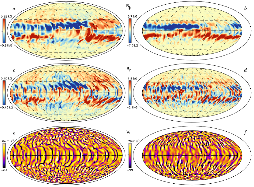
Figure 2.— Magnetic wreaths and convective flows sampled at the same instant in case D3. $(a)$ Longitudinal magnetic field $B_{\phi}$ near the top of the shell ($0.95R_{\odot}$) and ($b$) at mid-depth ($0.85R_{\odot}$). Strong flux structures with opposite polarity lie above and below the equator and span the convection zone. ($c,d$) Weaker radial magnetic field $B_{r}$ permeates and encircles each wreath. ($e,f$) Strong convective upflows and downflows shown by $V_{r}$ pass through and around the wreaths. The regions of strong magnetism tend to disrupt the convective flows while the strongest downflows serve to pump the wreaths to greater depths.

To initiate our dynamo case, a small seed dipole magnetic field was introduced and evolved via the induction equation. The energy in the magnetic fields is initially many orders of magnitude smaller than the energy contained in the convective motions, but these fields are amplified by shear and grow to become comparable in energy to the convective motions.

Stellar dynamo simulations are computationally intensive, requiring both high resolutions to correctly represent the velocity fields and long time evolution to capture the equilibrated dynamo behavior, which may include cyclic variations on time scales of several years. The strong magnetic fields can produce rapidly moving Alfvén waves which seriously restrict the Courant-Friedrichs-Lewy (CFL) timestep limits in the upper portions of the convection zone. Case D3, rotating three times faster than the current Sun, has been evolved for over 7000 days (or over 2 million timesteps). We plan to report on a variety of other dynamo cases, some at higher turbulence levels and rotation rates, in subsequent papers.

This dynamo simulation was conducted at magnetic Prandtl number $\mathrm{Pm}=\nu/\eta=0.5$, a value significantly lower than employed in our previous solar simulations. In particular, Brun et al. (2004) explored $\mathrm{Pm}=2,2.5$ and $4$, and Browning et al. (2006) studied $\mathrm{Pm}=8$. The high magnetic Prandtl numbers were required in the solar simulations to reach sufficiently high magnetic Reynolds numbers to drive sustained dynamo action. In the simulations of Brun et al. (2004) only the simulations with $\mathrm{Pm}>2.5$ and $\mathrm{Rm}^{\prime}\gtrsim 300$ achieved sustained dynamo action, where $\mathrm{Rm}^{\prime}$ is the fluctuating magnetic Reynolds number. We are here able to use a lower magnetic Prandtl number for three reasons. Firstly, more rapid rotation tends to stabilize convection and lower values of $\nu$ and $\eta$ are required to drive the convection. Once convective motions begin, they become quite vigorous and the fluctuating velocities saturate at values comparable to our solar cases. Thus the Reynolds numbers achieved are fairly large and we can achieve modestly high magnetic Reynolds numbers even at low $\mathrm{Pm}$. Secondly, the differential rotation becomes substantially stronger with both more rapid rotation $\Omega_{0}$ and with lower diffusivities $\nu$ and $\eta$. This global-scale flow is an important ingredient and reservoir of energy for these dynamos, and the increase in its amplitude means that low $\mathrm{Pm}$ dynamos can still achieve large magnetic Reynolds numbers based on this zonal flow. Lastly, the critical magnetic Reynolds number for dynamo action likely decreases with increasing kinetic helicity (e.g., Leorat et al. 1981), and helicity generally increases with rotation rate (e.g., Käpylä et al. 2009). Indeed there are even suggestions that the presence of a mean shearing flow may lower the critical magnetic Reynolds number (Hughes & Proctor 2009), and the strong differential rotation present in these rapidly rotating suns may serve to lower this threshold for dynamo action. We find that the rapidly rotating flows considered here achieve dynamo action at somewhat lower $\mathrm{Rm}$ than the models of Brun et al. (2004), which rotated at the solar rate.

3. Dynamos with Persistent Magnetic Wreaths

We here explore case D3 which yields fairly persistent wreaths of magnetism in its two hemispheres, though these do wax and wane somewhat in strength once established. Examining the properties of this dynamo solution should help to provide a perspective for the greater variations realized in our time-dependent dynamos which will be discussed in a following paper.

3.1. Patterns of Convection

The complex and evolving convective structures in our dynamo cases are substantially similar to the patterns of convection found in our hydrodynamic simulations. Our dynamo solution rotating at three times the solar rate, case D3, is presented in Figure 1, along with its hydrodynamic progenitor, case H3. The radial velocities shown near the top of the simulated domain (Figs. 1$a,e$) have broad upflows and narrow downflows as a consequence of the compressible motions. Near the equator the convection is aligned largely in the north-south direction, and these broad fronts sweep through the domain in a prograde fashion. The strongest downflows penetrate to the bottom of the convection zone; the weaker flows are partially truncated by the strong zonal flows of differential rotation. In the polar regions the convection is more isotropic and cyclonic. There the networks of downflow lanes surround upflows and both propagate in a retrograde fashion.

The convection establishes a prominent differential rotation profile by redistributing angular momentum and entropy, building gradients in latitude of angular velocity and temperature. Figures 1$b,f$ show the mean angular velocity $\Omega(r,\theta)$ for cases D3 and H3, revealing a solar-like structure with a prograde (fast) equator and retrograde (slow) pole. Figures 1$c,g$ present in turn radial cuts of $\Omega$ at selected latitudes, which are useful as we consider the angular velocity patterns realized here with faster rotation. These $\Omega(r,\theta)$ profiles are averaged in azimuth (longitude) and time over a period of roughly 200 days. Contours of constant angular velocity are aligned nearly on cylinders, influenced by the Taylor-Proudman theorem.

In the Sun, helioseismology has revealed that the contours of angular velocity are aligned almost on radial lines rather than on cylinders. The tilt of $\Omega$ contours in the Sun may be due in part to the thermal structure of the solar tachocline, as first found in the mean-field models of Rempel (2005) and then in 3D simulations of global-scale convection by Miesch et al. (2006). In those computations, it was realized that introducing a weak latitudinal gradient of entropy at the base of the convection zone, consistent with a thermal wind balance in a tachocline of shear, can serve to tilt the $\Omega$ contours toward a more radial alignment without significantly changing either the overall $\Omega$ contrast with latitude or the convective patterns. Ballot et al. (2007) explored the consequences of such a boundary condition in one of their simulations of young, rapidly rotating suns with deep convection zones and found that the effects on the differential rotation were similar to those found in Miesch et al. (2006). We expect similar behavior here, but at present observations of rapidly rotating stars only measure differential rotation at the surface and do not offer constraints on either the existence of tachoclines in young suns or the nature of their internal differential rotation profiles. As such, we have neglected the possible tachoclines of penetration and shear entirely in these models and instead adopt the simplification of imposing a constant radial entropy gradient at the bottom of the convection zone.

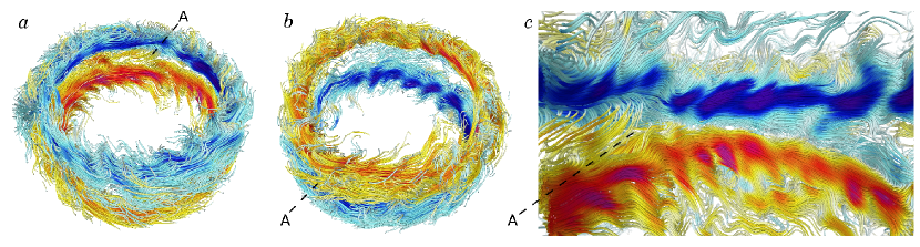
Figure 3.— Field line tracings of magnetic wreaths in case D3. $(a)$ Snapshot of two wreaths in full volume at same instant as in Fig. 2. Lines trace the magnetic fields, color denoting the amplitude and polarity of the longitudinal field $B_{\phi}$ (red, positive; blue, negative). Magnetic field threads in and out of the wreaths, connecting the two opposite polarity structures across the equator (i.e., region A) and to the polar regions where the magnetic field is wound up by the cyclonic convection. $(b)$ Same snapshot showing south polar region. $(c)$ Zoom in on region A showing the complex interconnections across the equator between the two wreaths and to high latitudes. Convective flows create the distinctive waviness visible in all three images.

Table 2Near-surface $\Delta\Omega$

Case	$\Delta\Omega_{\mathrm{lat}}$	$\Delta\Omega_{\mathrm{r}}$	$\Delta\Omega_{\mathrm{lat}}/\Omega_{\mathrm{eq}}$	Epoch
D3	1.18	0.71	0.137	2010-6980
H3	2.22	0.94	0.246	-

Note. — Angular velocity shear in units of $\mu\mathrm{rad}\>s^{-1}$, with $\Delta\Omega_{\mathrm{lat}}$ measured near the surface ($0.97R_{\odot}$) and $\Delta\Omega_{\mathrm{r}}$ measured across the full shell at the equator. The relative latitudinal shear $\Delta\Omega_{\mathrm{lat}}/\Omega_{\mathrm{eq}}$ is also measured at the same point near the surface. For the dynamo case, these measurements are taken over the indicated range of days. Case D3 shows slow variations in $\Delta\Omega_{\mathrm{lat}}$ over periods of about 2000 days. The hydrodynamic case is averaged for roughly 300 days and shows no systematic variation on longer timescales.

The differential rotation achieved is stronger in our hydrodynamic case H3 than in our dynamo case D3. This can be quantified by measurements of the latitudinal angular velocity shear $\Delta\Omega_{\mathrm{lat}}$. Here, as in Brown et al. (2008), we define $\Delta\Omega_{\mathrm{lat}}$ as the shear near the surface between the equator and a high latitude, say $\pm 60^{\circ}$

$$\Delta\Omega_{\mathrm{lat}}=\Omega_{\mathrm{eq}}-\Omega_{60},$$ (12)

and the radial shear $\Delta\Omega_{\mathrm{r}}$ as the angular velocity shear between the surface and bottom of the convection zone near the equator

$$\Delta\Omega_{\mathrm{r}}=\Omega_{0.97R_{\odot}}-\Omega_{0.72R_{\odot}}.$$ (13)

We further define the relative shear as $\Delta\Omega_{\mathrm{lat}}/\Omega_{\mathrm{eq}}$. In both definitions, we average the measurements of $\Delta\Omega$ in the northern and southern hemispheres, as the rotation profile is often slightly asymmetric about the equator. Case H3 achieves an absolute contrast $\Delta\Omega_{\mathrm{lat}}$ of 2.22 $\mu~{}\mathrm{rad}\>\mathrm{s}^{-1}$ (352 nHz) and a relative contrast of 0.247. The strong global-scale magnetic fields realized in the dynamo case D3 serve to diminish the differential rotation. As such, this case achieves an absolute contrast $\Delta\Omega_{\mathrm{lat}}$ of only 1.18 $\mu~{}\mathrm{rad}\>\mathrm{s}^{-1}$ (188 nHz) and a relative contrast of 0.137. This results from both a slowing of the equatorial rotation rate and an increase in the rotation rate in the polar regions. These results are quoted in Table 2.

The meridional circulations realized in the dynamo case D3 are very similar to those found in its hydrodynamic progenitor (case H3). As illustrated in Figures 1$d,h$, the circulations are multi-celled in radius and latitude. The cells are strongly aligned with the rotation axis, though some flows along the inner and outer boundaries cross the tangent cylinder and serve to weakly couple the polar regions to the equatorial convection. Flows of meridional circulation are slightly stronger in the dynamo cases than in the purely hydrodynamic cases, though both cases have weaker flows than are found in simulations rotating at the solar rate. Thus, as found in Brown et al. (2008), the flows of meridional circulation appear to weaken with more rapid rotation. The multi-celled nature of these meridional circulations may hold implications for flux transport dynamo models (e.g, Jouve & Brun 2007). Recent mean-field dynamo models are also beginning to explore the implications of weaker and multi-celled meridional circulations for dynamo action in more rapidly rotating suns (e.g., Jouve et al. 2009).

3.2. Kinetic and Magnetic Energies

Convection in these rapidly rotating dynamos is responsible for building the differential rotation and the magnetic fields. In a volume averaged sense, the energy contained in the magnetic fields in case D3 is about 10% of the kinetic energy. About 35% of this kinetic energy is contained in the fluctuating convection (CKE) and about 65% in the differential rotation (DRKE), whereas the weaker meridional circulations contain only a small portion (MCKE). The magnetic energy is split between the contributions from fluctuating fields (FME), involving roughly 53% of the total magnetic energy, and the energy of the mean toroidal fields (TME) that are 43% of the total. The energy contained in the mean poloidal fields (PME) is only 4% of the total magnetic energy. These energies are defined as

$$\mathrm{CKE} = \frac{1}{2}\bar{\rho}\Big{[}\left(v_{r}-\langle v_{r}\rangle\right)^{2}+\left(v_{\theta}-\langle v_{\theta}\rangle\right)^{2}+$$ (14)

$$\qquad\left(v_{\phi}-\langle v_{\phi}\rangle\right)^{2}\Big{]},$$

$$\mathrm{DRKE} = \frac{1}{2}\bar{\rho}\langle v_{\phi}\rangle^{2},$$ (15)

$$\mathrm{MCKE} = \frac{1}{2}\bar{\rho}\Big{(}\langle v_{r}\rangle^{2}+\langle v_{\theta}\rangle^{2}\Big{)},$$ (16)

$$\mathrm{FME} = \frac{1}{8\pi}\Big{[}\left(B_{r}-\langle B_{r}\rangle\right)^{2}+\left(B_{\theta}-\langle B_{\theta}\rangle\right)^{2}+$$ (18)

$$\qquad\left(B_{\phi}-\langle B_{\phi}\rangle\right)^{2}\Big{]},$$

$$\mathrm{TME} = \frac{1}{8\pi}\langle B_{\phi}\rangle^{2},$$ (19)

$$\mathrm{PME} = \frac{1}{8\pi}\Big{(}\langle B_{r}\rangle^{2}+\langle B_{\theta}\rangle^{2}\Big{)}.$$ (20)

where angle brackets denote an average in longitude.

These results are in contrast to our previous simulations of the solar dynamo, where the mean fields contained only about 2% of the magnetic energy and the fluctuating fields contained nearly 98% (Brun et al. 2004). In simulations of the solar dynamo that included a stable tachocline at the base of the convection zone (Browning et al. 2006), the energy of the mean fields in the tachocline can exceed the energy of the fluctuating fields there by about a factor of three, though the fluctuating fields still dominate the magnetic energy budget within the convection zone itself. Simulations of dynamo activity in the convecting cores of A-type stars (Brun et al. 2005) achieved similar results. There in the stable radiative zone the energies of the mean fields were able to exceed the energy contained in the fluctuating fields, but in the convecting core the fluctuating fields contained roughly 95% of the magnetic energy. Simulations of dynamo action in fully-convective M-stars do however show high levels of magnetic energy in the mean fields (Browning 2008). In those simulations the fluctuating fields still contain much of the magnetic energy, but the mean toroidal fields possess about 18% of the total throughout most of the stellar interior. In our rapidly rotating suns, the mean fields comprise a significant portion of the magnetic energy in the convection zone and are as important as the fluctuating fields.

Convection is similarly strong in both rapidly rotating cases, and CKE is similar in magnitude. The differential rotation in the dynamo case is much weaker than in the hydrodynamic progenitor, and DRKE has decreased by about a factor of five. Meridional circulations are comparably weak in both cases.

Table 3Energies

Case	CKE	DRKE	MCKE	FME	TME	PME
D3	$2.31$	$4.35$	$0.010$	$0.36$	$0.29$	$0.029$
H3	$2.56$	$22.2\phantom{0}\phantom{0}$	$0.012$	-	-	-

Note. — Volume-averaged energy densities relative to the rotating coordinate system. Kinetic energies are shown for convection (CKE), differential rotation (DRKE) and meridional circulations (MCKE). Magnetic energies are shown for fluctuating magnetic fields (FME), mean toroidal fields (TME) and mean poloidal fields (PME). All energy densities are reported in units of $10^{6}\mathrm{erg}\>\mathrm{cm}^{-3}$ and are averaged over 1000 day periods.

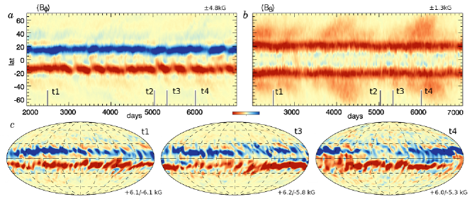
Figure 4.— Persistent wreaths of magnetism in case D3. $(a)$ Time-latitude plots of azimuthally-averaged longitudinal field $\langle B_{\phi}\rangle$ at mid-convection zone ($0.85R_{\odot}$) in a view spanning latitudes from $\pm 70^{\circ}$, with scaling values indicated. The two wreaths of opposite polarity persist for more than 4000 days. $(b)$ Mean colatitudinal magnetic field $\langle B_{\theta}\rangle$ at mid-convection zone over same interval. $(c)$ Snapshots of $B_{\phi}$ in Mollweide projection at mid-convection zone, shown for three times indicated in $a,b$. The wreaths maintain constant polarity over long time intervals, but still show variation as they interact with the convection. Time t2 corresponds to the snapshot in Fig. 2$b$.

4. Wreaths of Magnetism

These rapidly rotating dynamos produce striking magnetic structures in the midst of their turbulent convection zones. The magnetic field is organized into large banded, wreath-like structures positioned near the equator and spanning the depth of the convection zone. These wreaths are shown for case D3 at two depths in the convection zone in Figure 2. The dominant component of the magnetic wreaths is the strong longitudinal field $B_{\phi}$, with each wreath possessing its own polarity. The average strength of the longitudinal field at mid-convection zone is $\pm 7$ kG and peak field strengths there reach roughly $\pm 26$ kG. Threaded throughout the wreaths are weaker radial and latitudinal magnetic fields, which connect the two structures across the equator and also to the high-latitude regions.

These wreaths of magnetism survive despite being embedded in vigorous convective upflows and downflows. The convective flows leave their imprint on the magnetic structures, with individual downflow lanes entraining the magnetic field, advecting it away, and stretching it into $B_{r}$ while leaving regions of locally reduced $B_{\phi}$. The slower upflows carry stronger $B_{\phi}$ up from the depths. Where the magnetism is particularly strong the convective flows are disrupted. Meanwhile, where the convective flows are strongest, the longitudinal magnetic field is weakened and appears to vanish. In reality, the magnetic wreaths here are diving deeper below the mid-convection zone, apparently pumped down by the pummeling action of the strong downflows.

The deep structure of these wreaths is revealed by field line tracings throughout the volume, shown in Figure 3 for the same instant in time. The wreaths are topologically leaky structures, with magnetic field lines threading in and out of the surrounding convection. The wreaths are connected to the high-latitude (polar) convection, and on the poleward edges they show substantial winding from the highly vortical convection found there. This occurs in both the northern and southern hemispheres, as shown in two views at the same instant (north, Fig. 3$a$ and south, Fig. 3$b$). It is here that the global-scale poloidal field is being regenerated by the coupling of fluctuating velocities and fluctuating fields. Magnetic fields cross the equator, tying the two wreaths together at many locations (Fig. 3$c$). The strongest convective downflows leave their imprint on the wreaths as regions where the field lines are dragged down deeper into the convection zone, yielding a wavy appearance to the wreaths as a whole.

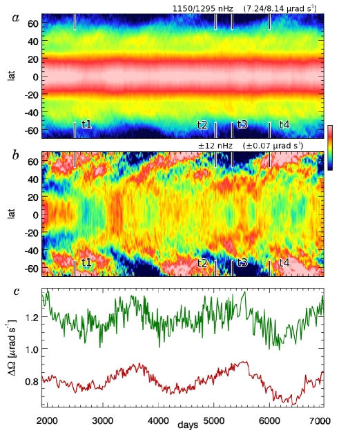
Figure 5.— Differential rotation in case D3. $(a)$ Angular velocity $\Omega$ at mid-convection zone ($0.85R_{\odot}$), with ranges in both nHz and $\mu\mathrm{rad}\>\mathrm{s}^{-1}$. The equator is fast while the poles rotate more slowly. $(b)$ Temporal variations are emphasized by subtracting the time-averaged profile of $\Omega(r,\theta)$, revealing speedup structures at high latitudes and pulses of fast and slow motion near the equator. $(c)$ Angular velocity shear $\Delta\Omega_{\mathrm{lat}}$ (eq. 12) near the surface (upper curve, green) and at mid-convection zone (lower, red).

4.1. Wreaths Persist for Long Epochs

The wreaths of magnetism built in case D3 persist for long periods of time, with little change in strength and no reversals in global-scale polarity for as long as we have pursued these calculations. The long-term stability of the wreaths realized by the dynamo of case D3 is shown in Figure 4. Here the azimuthally-averaged longitudinal field $\langle B_{\phi}\rangle$ and colatitudinal field $\langle B_{\theta}\rangle$ are shown at mid-convection zone at a point after the dynamo has equilibrated and for a period of roughly 5000 days (i.e., several ohmic diffusion times). During this interval there is little change in either the amplitude or structure of the mean fields. This is despite the short overturn times of the convection (10-30 days) or the rotation period of the star ($\sim 9$ days). The ohmic diffusion time at mid-convection zone is approximately 1300 days.

Though the mean (global-scale) fields are roughly steady in nature (Figs. 4$a,b$), the magnetic field interacts strongly with the convection on smaller scales. Several samples of longitudinal field $B_{\phi}$ are shown in full Mollweide projection at mid-convection zone (Fig. 4$c$). The magnetic fields are clearly reacting on short time scales to the convection but the wreaths maintain their coherence.

There are also some small but repeated variations in the global-scale magnetic fields. Visible in Figure 4$b$ are events where propagating structures of $\langle B_{\theta}\rangle$ reach toward higher latitudes over periods of about 1000 days (i.e., from day 3700 to day 4500 and from day 5600 to day 6400). These are accompanied by slight variations in the volume-averaged magnetic energy densities and the comparable kinetic energy of the differential rotation. These variations are also visible in the differential rotation itself, as shown in Figure 5. The differential rotation is fairly stable, though some time variation is visible at high latitudes. This is better revealed (Fig. 5$b$) by subtracting the time-averaged profile of $\Omega$ at each latitude, revealing the temporal variations about this mean. In the polar regions above $\pm 40^{\circ}$ latitude, speedup features move poleward over 500 day periods. These features track similar structures visible in the mean magnetic fields (Fig. 4$b$). The bands of velocity speedup bear some resemblance to the poleward branch of torsional oscillations observed in the solar convection zone over the course of a solar magnetic activity cycle (e.g., Thompson et al. 2003; Howe 2009), though here they propagate to higher latitudes on a shorter time scale.

The temporal variations of the angular velocity contrast in latitude $\Delta\Omega_{\mathrm{lat}}$ are shown for this period in Figure 5$c$. At mid-convection zone (sampled by red line) the variations in $\Delta\Omega_{\mathrm{lat}}$ are modest, varying by roughly 8%. Near the surface (green line) $\Delta\Omega_{\mathrm{lat}}$ shows similar variations with amplitudes of about 6%. The near-surface values of $\Delta\Omega_{\mathrm{lat}}$ are reported in Table 2, averaged over this entire period.

These evolving structures of magnetism and faster and slower differential rotation appear to be the first indications of behavior where the mean fields themselves begin to wax and wane substantially in strength. As the magnetic Reynolds number is increased, by either decreasing the magnetic diffusivity $\eta$ or by increasing the rotation rate of the star $\Omega_{0}$, this time varying behavior becomes more prominent and can even result in organized changes in the global-scale polarity. Such behavior is evident in a number of our dynamo simulations and will be reported on in a subsequent paper.

5. Creating Magnetic Wreaths

The magnetic wreaths formed in case D3 are dominated by strong mean longitudinal field components and show little variation in time. To understand the physical processes responsible for maintaining these magnetic wreaths, we examine the terms arising in the time- and azimuth-averaged induction equation for case D3.

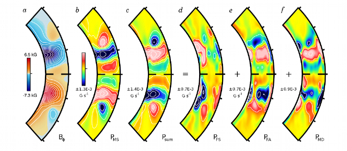
Figure 6.— Generation of mean toroidal magnetic field in case D3. The view is from $\pm 45^{\circ}$ latitude to emphasize the equatorial regions. $(a)$ Mean toroidal field $\langle B_{\phi}\rangle$ with wreaths strongly evident. $(b)$ Production by $P_{\mathrm{MS}}$ serves to build $\langle B_{\phi}\rangle$. This rate term generally matches the sense of $\langle B_{\phi}\rangle$, thus being negative (blue in colorbar, with ranges indicated) in the core of the northern wreath and positive (red) in that of the southern wreath. $(c)$ Destruction of mean toroidal field is achieved by the sum of the two fluctuating (turbulent) induction terms and the ohmic diffusion $\left(P_{\mathrm{FS}}+P_{\mathrm{FA}}+P_{\mathrm{MD}}\right)$. This sum clearly has opposite sense and similar magnitude to $P_{\mathrm{MS}}$. We break out these three destruction terms in the following panels. $(d)$ Fluctuating (turbulent) shear $P_{\mathrm{FS}}$ is strongest near the high-latitude side of each wreath, and $(e)$ fluctuating (turbulent) advection $P_{\mathrm{FA}}$ is strongest in the cores of the wreaths. The sum of these terms $\left(P_{\mathrm{FS}}+P_{\mathrm{FA}}\right)$ is responsible for about half the destructive balance, with the remainder coming from $(f)$ the mean ohmic diffusion $P_{\mathrm{MD}}$. Some differences arise in the boundary layers at top and bottom.

5.1. Maintaining Wreaths of Toroidal Field

We begin our analysis by exploring the maintenance of the mean toroidal field $\langle B_{\phi}\rangle$. Here it is helpful to break the induction term from equation (4) into contributions from shear, advection and compression, namely

$$\boldsymbol{\nabla} \boldsymbol{\times} \left(\boldsymbol{v}\boldsymbol{\times}\boldsymbol{B}\right)=$$ (21)

$$\underbrace{\left(\boldsymbol{B}\cdot\boldsymbol{\nabla}\right)\boldsymbol{v}}_{\mbox{shear}}-\underbrace{\left(\boldsymbol{v}\cdot\boldsymbol{\nabla}\right)\boldsymbol{B}}_{\mbox{advection}}-\underbrace{\boldsymbol{B}\left(\boldsymbol{\nabla}\cdot\boldsymbol{v}\right)}_{\mbox{compression}}.$$

Details of this decomposition are given in the Appendix.

The evolution of the mean longitudinal (toroidal) field $\langle B_{\phi}\rangle$ is described symbolically in equation (A8), with individual terms defined in equation (A9). When we analyze these terms in case D3, we find that $\langle B_{\phi}\rangle$ is produced by the shear of differential rotation and is dissipated by a combination of turbulent induction and ohmic diffusion. This balance can be restated as

$$\frac{\partial\langle B_{\phi}\rangle}{\partial t}\approx P_{\mathrm{MS}}+\left(P_{\mathrm{FS}}+P_{\mathrm{FA}}+P_{\mathrm{MD}}\right)\approx 0\thinspace,$$ (22)

with $P_{\mathrm{MS}}$ representing production by the mean shearing flow of differential rotation, $P_{\mathrm{FS}}$ by fluctuating shear, $P_{\mathrm{FA}}$ by fluctuating advection, and $P_{\mathrm{MD}}$ by mean ohmic diffusion. Those terms are in turn

$$P_{\mathrm{MS}} = \phantom{0}\left(\langle\boldsymbol{B}\rangle\cdot\boldsymbol{\nabla}\right)\langle\boldsymbol{v}\rangle\big{|}_{\phi},$$ (23)

$$P_{\mathrm{FS}} = \phantom{0}\left\langle\left(\boldsymbol{B}^{\prime}\cdot\boldsymbol{\nabla}\right)\boldsymbol{v^{\prime}}\right\rangle\big{|}_{\phi},$$ (24)

$$P_{\mathrm{FA}} = -\left\langle\left(\boldsymbol{v}^{\prime}\cdot\boldsymbol{\nabla}\right)\boldsymbol{B^{\prime}}\right\rangle\big{|}_{\phi},$$ (25)

$$P_{\mathrm{MD}} = -\boldsymbol{\nabla}\boldsymbol{\times}\eta\boldsymbol{\nabla}\boldsymbol{\times}\langle\boldsymbol{B}\rangle\big{|}_{\phi},$$ (26)

where brackets again indicate an azimuthal average and primes indicate fluctuating terms: $\boldsymbol{v}^{\prime}=\boldsymbol{v}-\langle\boldsymbol{v}\rangle$. The detailed implementation of these terms is presented for our spherical geometry in equations (A10-A15). These terms are illustrated in Figure 6 for case D3, averaged over a 450 day interval from day 6450 to 6900.

The structure of $\langle B_{\phi}\rangle$ is shown in Figure 6$a$. The shearing flows of differential rotation $P_{\mathrm{MS}}$ (Fig. 6$b$) act almost everywhere to reinforce the mean toroidal field. Thus the polarity of this production term generally matches that of $\langle B_{\phi}\rangle$. This production is balanced by destruction of mean field arising from both turbulent induction and ohmic diffusion (sum shown in Fig. 6$c$). The individual profiles of $P_{\mathrm{FS}}$, $P_{\mathrm{FA}}$ and $P_{\mathrm{MD}}$ are presented in turn in Figures 6$d,e,f$. The terms from turbulent induction ($P_{\mathrm{FS}}$ and $P_{\mathrm{FA}}$) contribute to roughly half of the total balance, with the remainder carried by ohmic diffusion of the mean fields ($P_{\mathrm{MD}}$). In the core of the wreaths, removal of mean toroidal field is largely accomplished by fluctuating advection $P_{\mathrm{FA}}$ (Fig. 6$e$) and mean ohmic diffusion $P_{\mathrm{MD}}$ (Fig. 6$f$), with the latter also important near the upper boundary. Turbulent shear becomes strongest near the bottom of the convection zone and in the regions near the high-latitude side of each wreath. Thus $P_{\mathrm{FS}}$ (Fig. 6$d$) becomes the dominant member of the triad of terms seeking to diminish the mean toroidal field there. We find that the mean poloidal field is regenerated in roughly the same region.

In the analysis presented in Figure 6 we have neglected the advection of $\langle B_{\phi}\rangle$ by the meridional circulations (shown in the Appendix as $P_{\mathrm{MA}}$), which we find plays a very small role in the overall balance. We have also neglected the amplification of $\langle B_{\phi}\rangle$ by compressibility effects (the Appendix, $P_{\mathrm{MC}}$ and $P_{\mathrm{FC}}$), though it does contribute slightly to reinforcing the underlying mean fields within the wreaths.

To summarize, the mean toroidal fields are built through an $\Omega$-effect, where production by the mean shearing flow of differential rotation ($P_{\mathrm{MS}}$) builds the underlying $\langle B_{\phi}\rangle$. In the statistically steady state achieved, this production is balanced by a combination of turbulent induction ($P_{\mathrm{FS}}+P_{\mathrm{FA}}$) and ohmic diffusion of the mean fields ($P_{\mathrm{MD}}$).

5.2. Maintaining the Poloidal Field

The production of mean poloidal field is achieved through a slightly different balance, with turbulent induction producing poloidal field and ohmic diffusion acting to dissipate it. The mean flows play little role in the overall balance. This balance is clarified if we represent the mean poloidal field by its vector potential $\langle A_{\phi}\rangle$, where

$$\langle\boldsymbol{B}_{\mathrm{pol}}\rangle=\langle B_{r}\rangle\boldsymbol{\hat{r}}+\langle B_{\theta}\rangle\boldsymbol{\hat{\theta}}=\boldsymbol{\nabla}\boldsymbol{\times}\left\langle A_{\phi}\boldsymbol{\hat{\phi}}\right\rangle,$$ (27)

as discussed in the Appendix. We recast the induction equation (4) in terms of the poloidal vector potential by uncurling the equation once, obtaining

$$\frac{\partial\langle\boldsymbol{A_{\phi}}\rangle}{\partial t}=\left\langle\boldsymbol{v}\boldsymbol{\times}\boldsymbol{B}\right\rangle{\big{|}}_{\phi}-\eta\boldsymbol{\nabla}\boldsymbol{\times}\left\langle\boldsymbol{B}\right\rangle{\big{|}}_{\phi},$$ (28)

which is also equation (A29) in the Appendix. The first term is the electromotive force (emf) arising from the coupling of flows and magnetic fields, and the second term is the ohmic diffusion. These can be decomposed into contributions from mean and fluctuating components, as shown symbolically in equation (A30).

In case D3 we find that the mean poloidal vector potential $\langle A_{\phi}\rangle$ is produced by the fluctuating (turbulent) emf and is dissipated by ohmic diffusion

$$\frac{\partial\langle A_{\phi}\rangle}{\partial t}\approx E_{\mathrm{FI}}+E_{\mathrm{MD}}\approx 0\thinspace.$$ (29)

with $E_{\mathrm{FI}}$ the emf arising from fluctuating flows and fluctuating fields, and contributing to the mean induction. The $E_{\mathrm{MD}}$ is the emf arising from mean ohmic diffusion. These terms are

$$E_{\mathrm{FI}} = \langle\boldsymbol{v^{\prime}}\boldsymbol{\times}\boldsymbol{B^{\prime}}\rangle{\big{|}}_{\phi}=\langle v_{r}^{\prime}B_{\theta}^{\prime}\rangle-\langle v_{\theta}^{\prime}B_{r}^{\prime}\rangle,$$ (30)

$$E_{\mathrm{MD}} = -\eta\boldsymbol{\nabla}\boldsymbol{\times}\langle\boldsymbol{B}\rangle{\big{|}}_{\phi}.$$ (31)

The contribution arising from the omitted term $E_{\mathrm{MI}}$ (see eq. A31), related to the emf of mean flows and mean fields, is smaller than these first two by more than an order of magnitude. Additionally, $E_{\mathrm{MI}}$ has a complicated spatial structure which does not appear to act in a coherent fashion within the wreaths to either build or destroy mean poloidal field.

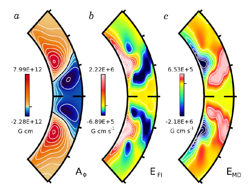
Figure 7.— Production of mean poloidal vector potential $\langle A_{\phi}\rangle$ in case D3, with view restricted to $\pm 45^{\circ}$ latitude. $(a)$ Mean poloidal vector potential $\langle A_{\phi}\rangle$, with sense denoted by color (red, clockwise; blue, counter-clockwise). $(b)$ The fluctuating (turbulent) emf $E_{\mathrm{FI}}$ acts to build the vector potential. This term is strongest near the bottom of the convection zone and the poleward side of the wreaths. $(c)$ Mean ohmic diffusion $E_{\mathrm{MD}}$ acts everywhere in opposition to $E_{\mathrm{FI}}$. The cores of the wreaths are positioned at roughly $\pm 15^{\circ}$ latitude (Fig. 6$a$).

The mean vector potential $\langle A_{\phi}\rangle$ is shown in Figure 7$a$, with poloidal field lines represented by the overlying contours. The mean radial magnetic field $\langle B_{r}\rangle$ is about $\pm 1$ kG in the cores of the wreaths, whereas the mean colatitudinal field $\langle B_{\theta}\rangle$ has an amplitude of roughly $-2$ kG (thus directed northward in both hemispheres), concentrated near the bottom of the convection zone.

The production of $\langle A_{\phi}\rangle$ by the fluctuating (turbulent) emf $E_{\mathrm{FI}}$ is shown in Figure 7$b$. Here too we average over the same 450 day interval. This term generally acts to reinforce the existing poloidal field, having the same sense as the underlying vector potential in most regions. It is strongest near the bottom of the convection zone and is concentrated at the poleward side of each wreath. This is similar, though not identical, to the structure of destruction of mean toroidal field by fluctuating shear $P_{\mathrm{FS}}$ (Fig. 6$d$). It suggests that mean toroidal field is here being converted into mean poloidal field by the fluctuating flows.

There are two terms that contribute to $E_{\mathrm{FI}}$, as shown in equation (30). Much of that fluctuating emf arises from correlations between fluctuating latitudinal flows and radial fields $\langle-v_{\theta}^{\prime}B_{r}^{\prime}\rangle$, which follows the structure of $E_{\mathrm{FI}}$ (Fig. 7$b$) closely. The contribution from fluctuating radial flows and colatitudinal fields $\langle v_{r}^{\prime}B_{\theta}^{\prime}\rangle$ is more complex in structure. Near $\pm 20^{\circ}$ latitude, this term reinforces $\langle-v_{\theta}^{\prime}B_{r}^{\prime}\rangle$, but acts against it at higher latitudes and thus diminishes the overall amplitude of $E_{\mathrm{FI}}$. The mean ohmic diffusion $E_{\mathrm{MD}}$ (Fig. 7$c$), almost entirely balances the production of $\langle A_{\phi}\rangle$ by $E_{\mathrm{FI}}$.

This shows that our mean poloidal magnetic field is maintained by the fluctuating (turbulent) emf and is destroyed by ohmic diffusion. In mean-field dynamo theory, this is often parametrized by an “$\alpha$-effect.” Now we turn to interpretations within that framework.

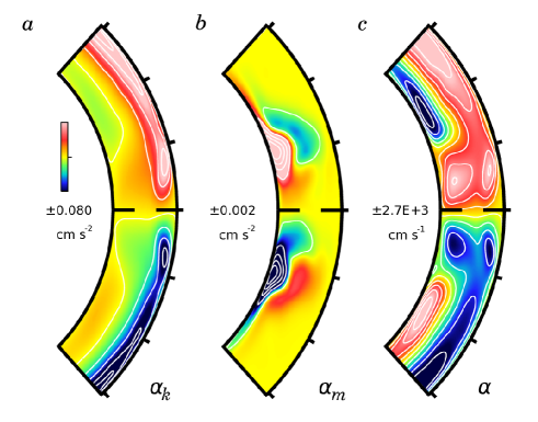
Figure 8.— Estimating the mean-field $\alpha$-effect from case D3. Shown are the $(a)$ kinetic and $(b)$ magnetic contributions to the $\alpha$-effect as defined in eqs. (33-35). $(c)$ Mean-field $\alpha$, constructed by combining $\alpha_{k}$ and $\alpha_{m}$ with a turbulent correlation time $\tau$.

6. Exploring Mean-Field Interpretations

Many mean-field theories assert that the production of mean poloidal field is likely to arise from the fluctuating emf. This process is often approximated with an $\alpha$-effect, where it is proposed that the sense and amplitude of the emf scales with the mean toroidal field

$$\langle\boldsymbol{v^{\prime}}\boldsymbol{\times}\boldsymbol{B^{\prime}}\rangle=\alpha\langle\boldsymbol{B}\rangle,$$ (32)

where $\alpha$ can be either a simple scalar or may be related to the kinetic and magnetic (current) helicities. In isotropic (but not reflectionally symmetric), homogeneous, incompressible MHD turbulence

$$\alpha = \phantom{0}\frac{\tau}{3}\left(\alpha_{k}+\alpha_{m}\right),$$ (33)

$$\alpha_{k} = -\boldsymbol{v^{\prime}}\cdot\left(\boldsymbol{\nabla}\boldsymbol{\times}\boldsymbol{v^{\prime}}\right),$$ (34)

$$\alpha_{m} = \phantom{0}\frac{1}{4\pi\rho}\boldsymbol{B^{\prime}}\cdot\left(\boldsymbol{\nabla}\boldsymbol{\times}\boldsymbol{B^{\prime}}\right),$$ (35)

as discussed in Pouquet et al. (1976) and Brandenburg & Subramanian (2005). Here $\tau$ is the lifetime or correlation time of a typical turbulent eddy. In mean-field theory, these fluctuating helicities are typically not solved directly and are instead solved through auxiliary equations for the total magnetic helicity or are prescribed. Here we can directly measure our fluctuating helicities and examine whether they approximate our fluctuating emf.

To assess the possible role of an $\alpha$-effect in our simulation, we show in Figures 8$a,b$ the fluctuating kinetic and current helicities $\alpha_{k}$ and $\alpha_{m}$ realized in our case D3, averaged over the same 450 day analysis interval. To make an estimate of the $\alpha$-effect, we approximate the correlation time $\tau$ by defining

$$\tau=\frac{H_{P}}{v^{\prime}}$$ (36)

where $H_{P}$ is the local pressure scale height and $v^{\prime}$ is the local fluctuating rms velocity, which are functions of radius only. Estimated by this method, the turnover time $\tau$ has a smooth radial profile and is roughly 10 days near the bottom of the convection zone, 3 days at mid-convection zone, and slightly less near the upper boundary. If we use the fast peak upflow or downflow velocities instead of the rms velocities, our estimate of $\tau$ is about a factor of 4 smaller. Our mean-field $\alpha$ (eq. 33) is shown in Figure 8$c$. In the upper convection zone, this is dominated by the fluctuating kinetic helicity while the fluctuating magnetic (current) helicity becomes important at depth.

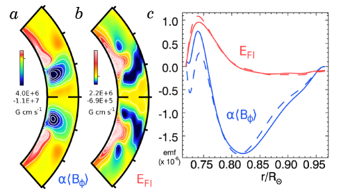
Figure 9.— Comparison of emfs in case D3. $(a)$ Profile of proposed mean-field emf given by $\alpha\langle B_{\phi}\rangle$. $(b)$ Actual turbulent emf $E_{\mathrm{FI}}$ measured in the dynamo. $(c)$ Variation of hemisphere-averaged emfs with fractional radius. The mean-field approximated emf is shown in blue, and $E_{\mathrm{FI}}$ in red. The average over the northern hemisphere is shown solid, the southern is dashed.

We form a mean-field emf (right-hand side of eq. 32) by multiplying our derived $\alpha$ (Fig. 8$c$) with our $\langle B_{\phi}\rangle$ (Fig. 6$a$), and show this in Figure 9$a$. The turbulent emf $E_{\mathrm{FI}}$, which is the left-hand side of equation (32), can be measured in our simulations and is shown again in Figure 9$b$. Although there is some correspondence in the two patterns, there are significant differences. In particular, the mean-field emf $\alpha\langle B_{\phi}\rangle$ has peak amplitudes in the cores of the wreaths (at $\pm 15^{\circ}$ latitude) and is negative there. In contrast, the actual fluctuating emf given by $E_{\mathrm{FI}}$ is positive and has its highest amplitude at the poleward side of the wreaths (near $\pm 20^{\circ}$ latitude). Thus the mean-field emf predicts an incorrect balance in the generation terms and would yield a distinctly different mean poloidal magnetic field.

To assess whether better agreement may be achieved with a latitude-averaged emf, we average the mean-field emf and $E_{\mathrm{FI}}$ separately over the northern and southern hemispheres and plot these quantities in Figure 9$c$. Though both have a similar positive sense near the base of the convection zone, the hemisphere-averaged $E_{\mathrm{FI}}$ becomes small above $0.8R_{\odot}$ whereas the averaged mean-field emf $\alpha\langle B_{\phi}\rangle$ is large and negative there. Thus even the averaged emfs are not in accord.

In summary, it is evident that a simple scalar $\alpha$-effect will predict the wrong sign for the fluctuating emf in the two hemispheres, as $\langle B_{\phi}\rangle$ is anti-symmetric across the equator while $\langle A_{\phi}\rangle$ is symmetric. An $\alpha$-effect based on the kinetic helicity and magnetic helicity may capture some sense of the fluctuating emf, as those quantities are themselves anti-symmetric across the equator. Yet Figure 9 suggests that there are significant discrepancies between this particular approximation and our turbulent emf. In particular, this mean-field $\alpha$-effect misses the offset between the generation regions for mean toroidal and mean poloidal field. This offset in latitude of the generation regions may be important for avoiding the $\alpha$-quenching problems encountered in many mean-field theories. A more complex mean-field model, which takes spatial gradients of $\langle B_{\phi}\rangle$ into account, may do better. In particular, the $\boldsymbol{\Omega}\boldsymbol{\times}\boldsymbol{J}$-effect (e.g., Moffatt & Proctor 1982; Rogachevskii & Kleeorin 2003) may be at work in these systems, and preliminary explorations indicate that this term matches the spatial structure of our $E_{\mathrm{FI}}$ better than the above $\alpha$-effect. A tensor representation of the $\alpha$-effect may also do much better at approximating $E_{\mathrm{FI}}$, and test-field techniques could be employed to measure this quantity e.g., Schrinner et al. 2005, and recently reviewed in Brandenburg 2009. As with our analysis of dynamo production terms presented in §5, this comparative study of $\alpha\langle B_{\phi}\rangle$ and $E_{\mathrm{FI}}$ is conducted here for the special circumstances of a dynamo which builds global-scale magnetic fields that are nearly steady in time. The magnetic wreaths realized in dynamos at higher magnetic Reynolds numbers show larger time-variations, and it is possible that $\alpha\langle B_{\phi}\rangle$ better approximates $E_{\mathrm{FI}}$ during the growing phase of each oscillation, when the magnetic fields have not yet saturated in strength and the dynamo is in a more kinematic regime.

7. Conclusions

The ability for a dynamo to build wreaths of strong magnetic fields in the bulk of the convection zone has largely been a surprise, for it had generally been supposed that turbulent convection would disrupt such magnetic structures. To avoid these difficulties, many solar and stellar dynamo theories shift the burden of magnetic storage, amplification and organization to a tachocline of shear and penetration at the base of the convection zone where motions are more quiescent. In contrast, our simulations of rapidly rotating stars are able to achieve sustained global-scale dynamo action within the convection zone itself, with the magnetic structures both being built and able to survive while embedded deep within the turbulence. These dynamos are able to circumvent the Parker instability by means of turbulent Reynolds and Maxwell stresses that contribute to the mechanical force balance and prevent the wreaths from buoyantly escaping the convection zone. This striking behavior may be enabled by the stars rotating somewhat faster than the current Sun, which yields a strong differential rotation that is a key element in the dynamo behavior. In our broader exploration of rapidly rotating dynamos, we find that magnetic wreaths are present in all simulations, including those rotating as slowly as $1.5\thinspace\Omega_{\odot}$. Such structures may be obtainable in simulations rotating at the solar rate as well, and efforts are underway to explore the presence of wreaths in solar dynamos.

We have achieved some dynamo states that are persistent and others that flip the sense of their magnetic fields. In our case D3 the global-scale fields have small vacillations in their amplitudes, but the magnetic wreaths retain their identities for many thousands of days. This represents hundreds of rotation periods and several magnetic diffusion times, indicating that the dynamo has achieved a persistent equilibrium.

Increasing the rotation rate or decreasing the magnetic diffusivity $\eta$ yields more complex time dependence. In many of our dynamos the oscillations can become large, and this may result in the global-scale fields repeatedly flipping their polarity. At times those dynamos appear to be cyclic but in other intervals they behave more chaotically. Such time-dependent dynamos will be reported on in a forthcoming paper. In separate explorations, we have found that magnetic wreaths also survive in the presence of a tachocline of penetration and shear. In those simulations the wreaths continue to fill the convection zone even while developing roots in the tachocline. Dynamos in rapidly rotating suns with tachoclines can also exhibit time-dependent oscillations and polarity reversals. Wreath-building dynamos with tachoclines will be reported on subsequently.

In our persistent case D3 we are able to analyze the generation and transport of mean magnetic field. We find that our dynamo action is of an $\alpha-\Omega$ nature, with the mean toroidal fields being generated by an $\Omega$-effect from the mean shearing flow of differential rotation. This generation is balanced by a combination of turbulent induction and ohmic diffusion. The mean poloidal fields appear to be generated by an $\alpha$-effect arising from couplings between the fluctuating flows and fluctuating fields, with this production largely balanced by the ohmic diffusion. This is unlike the toroidal balance, for here the mean flows play almost no role and the turbulent correlations are constructive rather than destructive. In assessing what a mean-field model might predict for the magnetic structures realized in case D3, we find that the isotropic, homogeneous $\alpha$-effect based on kinetic and magnetic (current) helicities fails to capture the sense of our turbulent emf. In general, our $E_{\mathrm{FI}}$ is poorly represented by an $\alpha\langle B_{\phi}\rangle$ that is so determined. This comparative analysis of $\alpha\langle B_{\phi}\rangle$ and $E_{\mathrm{FI}}$ is performed here only for the special case of a dynamo with persistent global-scale magnetic fields. It is possible that these results will differ in our dynamos that show substantial time-varying behavior.

The realization of global-scale magnetic structures in our simulations, and their great strength relative to the fluctuating fields, may in part be a consequence of the relatively modest degree of turbulence attained here. Whether such structures can be generated and sustained amidst the far more complex flows in actual stellar interiors is not yet clear. If such structures are indeed realized in stars, they may or may not survive to print through the highly turbulent convection occurring just below the stellar photosphere. If they do appear at the surface, some global-scale magnetic features may propagate toward the poles along with the bands of angular velocity speedup. There are some indications in stellar observations that global-scale toroidal magnetic fields may indeed become strong in rapidly rotating stars (Donati et al. 2006; Petit et al. 2008), though small-scale fields may still account for much of the magnetic energy near the surface (Reiners & Basri 2009). The global-scale poloidal fields may be more successful in surviving the passage through the turbulent surface convection. If they do, the stellar magnetic field will likely have significant non-dipole components. Thus the mean poloidal fields observed at the surface may give clues to the presence of large wreaths of magnetism that occupy the bulk of the convection zone.

Appendix A Production, Destruction and Transport of Magnetic Field

We derive diagnostic tools to evaluate the generation and transport of magnetic field in a magnetized and rotating turbulent convection zone. This derivation is in spherical coordinates, and is under the anelastic approximation.

A.1. Induction Equation

In the induction equation (4), the first term on the right hand side represents production of magnetic field while the second term represents its diffusion. We first rewrite the production term to make the contributions of shear, advection and compressible effects more explicit as

$$\mbox{\boldmath$\nabla$}\boldsymbol{\times}(\boldsymbol{v}\boldsymbol{\times}\boldsymbol{B})=(\boldsymbol{B}\cdot\mbox{\boldmath$\nabla$})\boldsymbol{v}-(\boldsymbol{v}\cdot\mbox{\boldmath$\nabla$})\boldsymbol{B}-\boldsymbol{B}(\mbox{$\boldsymbol{\nabla}\cdot\,$}\boldsymbol{v}).$$ (A1)

Under the anelastic approximation the divergence of $\boldsymbol{v}$ can be expressed in terms of the logarithmic derivative of the mean density because

$$\mbox{$\boldsymbol{\nabla}\cdot\,$}(\bar{\rho}\boldsymbol{v})=0=\bar{\rho}(\mbox{$\boldsymbol{\nabla}\cdot\,$}\boldsymbol{v})+(\boldsymbol{v}\cdot\mbox{\boldmath$\nabla$})\bar{\rho},$$

and therefore

$$\mbox{$\boldsymbol{\nabla}\cdot\,$}\boldsymbol{v}=-v_{r}\frac{\partial}{\partial r}\ln\bar{\rho}.$$ (A2)

The induction equation thus becomes

$$\frac{\partial\boldsymbol{B}}{\partial t}=\underbrace{(\boldsymbol{B}\cdot\mbox{\boldmath$\nabla$})\boldsymbol{v}}_{\mbox{shearing}}-\underbrace{(\boldsymbol{v}\cdot\mbox{\boldmath$\nabla$})\boldsymbol{B}}_{\mbox{advection}}+\underbrace{v_{r}\boldsymbol{B}\frac{\partial}{\partial r}\ln\bar{\rho}}_{\mbox{compression}}-\underbrace{\mbox{\boldmath$\nabla$}\boldsymbol{\times}(\eta\mbox{\boldmath$\nabla$}\boldsymbol{\times}\boldsymbol{B})}_{\mbox{diffusion}}$$ (A3)

As labeled, the first term represents shearing of $\boldsymbol{B}$, the second term advection of $\boldsymbol{B}$, the third one compressible amplification of $\boldsymbol{B}$, and the last term ohmic diffusion.

A.2. Production of Axisymmetric Magnetic Field

To identify the processes contributing to the production of mean (axisymmetric) field, we separate our velocities and magnetic fields into mean and fluctuating components $\boldsymbol{v}=\langle\boldsymbol{v}\rangle+\boldsymbol{v}^{\prime}$ and $\boldsymbol{B}=\langle\boldsymbol{B}\rangle+\boldsymbol{B}^{\prime}$ where angle brackets denote an average in longitude. Thus $\langle\boldsymbol{v}^{\prime}\rangle=\langle\boldsymbol{B}^{\prime}\rangle=0$ by definition. Expanding the production term of equation (A3) we obtain the mean shearing term

$$\langle(\boldsymbol{B}\cdot\mbox{\boldmath$\nabla$})\boldsymbol{v}\rangle=\left(\langle\boldsymbol{B}\rangle\cdot\mbox{\boldmath$\nabla$}\right)\langle\boldsymbol{v}\rangle+\langle(\boldsymbol{B}^{\prime}\cdot\mbox{\boldmath$\nabla$})\boldsymbol{v}^{\prime}\rangle,$$ (A4)

the mean advection term

$$-\langle(\boldsymbol{v}\cdot\mbox{\boldmath$\nabla$})\boldsymbol{B}\rangle=-\left(\langle\boldsymbol{v}\rangle\cdot\mbox{\boldmath$\nabla$}\right)\langle\boldsymbol{B}\rangle-\langle(\boldsymbol{v}^{\prime}\cdot\mbox{\boldmath$\nabla$})\boldsymbol{B}^{\prime}\rangle,$$ (A5)

and the mean compressibility term

$$\langle v_{r}\boldsymbol{B}\frac{\partial}{\partial r}\ln\bar{\rho}\rangle=\left(\langle v_{r}\rangle\langle\boldsymbol{B}\rangle+\langle v_{r}^{\prime}\boldsymbol{B}^{\prime}\rangle\right)\frac{\partial}{\partial r}\ln\bar{\rho}.$$ (A6)

In a similar fashion, the mean diffusion term becomes

$$-\langle\mbox{\boldmath$\nabla$}\boldsymbol{\times}(\eta\mbox{\boldmath$\nabla$}\boldsymbol{\times}\boldsymbol{B})\rangle=-\mbox{\boldmath$\nabla$}\boldsymbol{\times}(\eta\mbox{\boldmath$\nabla$}\boldsymbol{\times}\langle\boldsymbol{B}\rangle).$$ (A7)

The axisymmetric component of the induction equation is written symbolically as:

$$\frac{\partial\langle\boldsymbol{B}\rangle}{\partial t}=P_{\mathrm{MS}}+P_{\mathrm{FS}}+P_{\mathrm{MA}}+P_{\mathrm{FA}}+P_{\mathrm{MC}}+P_{\mathrm{FC}}+P_{\mathrm{MD}}$$ (A8)

With $P_{\mathrm{MS}}$ representing production of field by mean shear, $P_{\mathrm{FS}}$ production by fluctuating shear, $P_{\mathrm{MA}}$ advection by mean flows, $P_{\mathrm{FA}}$ advection by fluctuating flows, $P_{\mathrm{MC}}$ amplification arising from the compressibility of mean flows, $P_{\mathrm{FC}}$ amplification arising from fluctuating compressible motions, and $P_{\mathrm{MD}}$ ohmic diffusion of the mean fields. In turn, these terms are

$$P_{\mathrm{MS}}= \left(\langle\boldsymbol{B}\rangle\cdot\mbox{\boldmath$\nabla$}\right)\langle\boldsymbol{v}\rangle, P_{\mathrm{FS}}= \langle(\boldsymbol{B}^{\prime}\cdot\mbox{\boldmath$\nabla$})\boldsymbol{v}^{\prime}\rangle, P_{\mathrm{MA}}= -\left(\langle\boldsymbol{v}\rangle\cdot\mbox{\boldmath$\nabla$}\right)\langle\boldsymbol{B}\rangle, P_{\mathrm{FA}}= -\langle(\boldsymbol{v}^{\prime}\cdot\mbox{\boldmath$\nabla$})\boldsymbol{B}^{\prime}\rangle,$$

$$P_{\mathrm{MC}}= \left(\langle v_{r}\rangle\langle\boldsymbol{B}\rangle\right)\frac{\partial}{\partial r}\ln\bar{\rho}, P_{\mathrm{FC}}= \left(\langle v_{r}^{\prime}\boldsymbol{B}^{\prime}\rangle\right)\frac{\partial}{\partial r}\ln\bar{\rho},\text{and} P_{\mathrm{MD}}= -\mbox{\boldmath$\nabla$}\boldsymbol{\times}(\eta\mbox{\boldmath$\nabla$}\boldsymbol{\times}\langle\boldsymbol{B}\rangle).$$ (A9)

We now expand each of these terms into their full representation in spherical coordinates.

A.3. Production of Mean Longitudinal Field

$$\frac{\partial\langle B_{\phi}\rangle}{\partial t} = P_{\mathrm{MS}}+P_{\mathrm{FS}}+P_{\mathrm{MA}}+P_{\mathrm{FA}}+P_{\mathrm{MC}}+P_{\mathrm{FC}}+P_{\mathrm{MD}}$$

$$P_{\mathrm{MS}} = \phantom{0}\left[\langle B_{r}\rangle\frac{\partial}{\partial r}+\frac{\langle B_{\theta}\rangle}{r}\frac{\partial}{\partial\theta}\right]\langle v_{\phi}\rangle+\frac{\langle B_{\phi}\rangle\langle v_{r}\rangle+\cot\theta\langle B_{\phi}\rangle\langle v_{\theta}\rangle}{r}$$ (A10)

$$P_{\mathrm{FS}} = \phantom{0}\bigg{\langle}\left[B_{r}^{\prime}\frac{\partial}{\partial r}+\frac{B_{\theta}^{\prime}}{r}\frac{\partial}{\partial\theta}+\frac{B_{\phi}^{\prime}}{r\sin\theta}\frac{\partial}{\partial\phi}\right]v_{\phi}^{\prime}\bigg{\rangle}+\frac{\langle B_{\phi}^{\prime}v_{r}^{\prime}\rangle+\cot\theta\langle B_{\phi}^{\prime}v_{\theta}^{\prime}\rangle}{r}$$ (A11)

$$P_{\mathrm{MA}} = -\left[\langle v_{r}\rangle\frac{\partial}{\partial r}+\frac{\langle v_{\theta}\rangle}{r}\frac{\partial}{\partial\theta}\right]\langle B_{\phi}\rangle-\frac{\langle v_{\phi}\rangle\langle B_{r}\rangle+\cot\theta\langle v_{\phi}\rangle\langle B_{\theta}\rangle}{r}$$ (A12)

$$P_{\mathrm{FA}} = -\bigg{\langle}\left[v_{r}^{\prime}\frac{\partial}{\partial r}+\frac{v_{\theta}^{\prime}}{r}\frac{\partial}{\partial\theta}+\frac{v_{\phi}^{\prime}}{r\sin\theta}\frac{\partial}{\partial\phi}\right]B_{\phi}^{\prime}\bigg{\rangle}-\frac{\langle v_{\phi}^{\prime}B_{r}^{\prime}\rangle+\cot\theta\langle v_{\phi}^{\prime}B_{\theta}^{\prime}\rangle}{r}$$ (A13)

$$P_{\mathrm{MC}} = \phantom{0}\left(\langle v_{r}\rangle\langle B_{\phi}\rangle\right)\frac{\partial}{\partial r}\ln\bar{\rho}\qquad\qquad\qquad P_{\mathrm{FC}}=\left(\langle v_{r}^{\prime}B_{\phi}^{\prime}\rangle\right)\frac{\partial}{\partial r}\ln\bar{\rho}$$ (A14)

$$P_{\mathrm{MD}} = \phantom{0}\eta\nabla^{2}\langle B_{\phi}\rangle-\frac{\eta\langle B_{\phi}\rangle}{r^{2}\sin^{2}\theta}+\frac{d\eta}{dr}\left(\frac{1}{r}\frac{\partial(r\langle B_{\phi}\rangle)}{\partial r}\right)$$ (A15)

A.4. Production of Mean Latitudinal Field

$$\frac{\partial\langle B_{\theta}\rangle}{\partial t} = P_{\mathrm{MS}}+P_{\mathrm{FS}}+P_{\mathrm{MA}}+P_{\mathrm{FA}}+P_{\mathrm{MC}}+P_{\mathrm{FC}}+P_{\mathrm{MD}}$$

$$P_{\mathrm{MS}} = \phantom{0}\left[\langle B_{r}\rangle\frac{\partial}{\partial r}+\frac{\langle B_{\theta}\rangle}{r}\frac{\partial}{\partial\theta}\right]\langle v_{\theta}\rangle+\frac{\langle B_{\theta}\rangle\langle v_{r}\rangle-\cot\theta\langle B_{\phi}\rangle\langle v_{\phi}\rangle}{r}$$ (A16)

$$P_{\mathrm{FS}} = \phantom{0}\bigg{\langle}\left[B_{r}^{\prime}\frac{\partial}{\partial r}+\frac{B_{\theta}^{\prime}}{r}\frac{\partial}{\partial\theta}+\frac{B_{\phi}^{\prime}}{r\sin\theta}\frac{\partial}{\partial\phi}\right]v_{\theta}^{\prime}\bigg{\rangle}+\frac{\langle B_{\theta}^{\prime}v_{r}^{\prime}\rangle-\cot\theta\langle B_{\phi}^{\prime}v_{\phi}^{\prime}\rangle}{r}$$ (A17)

$$P_{\mathrm{MA}} = -\left[\langle v_{r}\rangle\frac{\partial}{\partial r}+\frac{\langle v_{\theta}\rangle}{r}\frac{\partial}{\partial\theta}\right]\langle B_{\theta}\rangle-\frac{\langle v_{\theta}\rangle\langle B_{r}\rangle-\cot\theta\langle v_{\phi}\rangle\langle B_{\phi}\rangle}{r}$$ (A18)

$$P_{\mathrm{FA}} = -\bigg{\langle}\left[v_{r}^{\prime}\frac{\partial}{\partial r}+\frac{v_{\theta}^{\prime}}{r}\frac{\partial}{\partial\theta}+\frac{v_{\phi}^{\prime}}{r\sin\theta}\frac{\partial}{\partial\phi}\right]B_{\theta}^{\prime}\bigg{\rangle}-\frac{\langle v_{\theta}^{\prime}B_{r}^{\prime}\rangle-\cot\theta\langle v_{\phi}^{\prime}B_{\phi}^{\prime}\rangle}{r}$$ (A19)

$$P_{\mathrm{MC}} = \phantom{0}\left(\langle v_{r}\rangle\langle B_{\theta}\rangle\right)\frac{\partial}{\partial r}\ln\bar{\rho}\qquad\qquad\qquad P_{\mathrm{FC}}=\phantom{0}\left(\langle v_{r}^{\prime}B_{\theta}^{\prime}\rangle\right)\frac{\partial}{\partial r}\ln\bar{\rho}$$ (A20)

$$P_{\mathrm{MD}} = \phantom{0}\eta\nabla^{2}\langle B_{\theta}\rangle+\frac{2\eta}{r^{2}}\frac{\partial\langle B_{r}\rangle}{\partial\theta}-\frac{\eta\langle B_{\theta}\rangle}{r^{2}\sin^{2}\theta}+\frac{d\eta}{dr}\left(\frac{1}{r}\frac{\partial(r\langle B_{\theta}\rangle)}{\partial r}-\frac{1}{r}\frac{\partial\langle B_{r}\rangle}{\partial\theta}\right)$$ (A21)

A.5. Production of Mean Radial Field

$$\frac{\partial\langle B_{r}\rangle}{\partial t} = P_{\mathrm{MS}}+P_{\mathrm{FS}}+P_{\mathrm{MA}}+P_{\mathrm{FA}}+P_{\mathrm{MC}}+P_{\mathrm{FC}}+P_{\mathrm{MD}}$$

$$P_{\mathrm{MS}} = \phantom{0}\left[\langle B_{r}\rangle\frac{\partial}{\partial r}+\frac{\langle B_{\theta}\rangle}{r}\frac{\partial}{\partial\theta}\right]\langle v_{r}\rangle-\frac{\langle B_{\theta}\rangle\langle v_{\theta}\rangle+\langle B_{\phi}\rangle\langle v_{\phi}\rangle}{r}$$ (A22)

$$P_{\mathrm{FS}} = \phantom{0}\bigg{\langle}\left[B_{r}^{\prime}\frac{\partial}{\partial r}+\frac{B_{\theta}^{\prime}}{r}\frac{\partial}{\partial\theta}+\frac{B_{\phi}^{\prime}}{r\sin\theta}\frac{\partial}{\partial\phi}\right]v_{r}^{\prime}\bigg{\rangle}-\frac{\langle B_{\theta}^{\prime}v_{\theta}^{\prime}\rangle+\langle B_{\phi}^{\prime}v_{\phi}^{\prime}\rangle}{r}$$ (A23)

$$P_{\mathrm{MA}} = -\left[\langle v_{r}\rangle\frac{\partial}{\partial r}+\frac{\langle v_{\theta}\rangle}{r}\frac{\partial}{\partial\theta}\right]\langle B_{r}\rangle+\frac{\langle v_{\theta}\rangle\langle B_{\theta}\rangle+\langle v_{\phi}\rangle\langle B_{\phi}\rangle}{r}$$ (A24)

$$P_{\mathrm{FA}} = -\bigg{\langle}\left[v_{r}^{\prime}\frac{\partial}{\partial r}+\frac{v_{\theta}^{\prime}}{r}\frac{\partial}{\partial\theta}+\frac{v_{\phi}^{\prime}}{r\sin\theta}\frac{\partial}{\partial\phi}\right]B_{r}^{\prime}\bigg{\rangle}+\frac{\langle v_{\theta}^{\prime}B_{\theta}^{\prime}\rangle+\langle v_{\phi}^{\prime}B_{\phi}^{\prime}\rangle}{r}$$ (A25)

$$P_{\mathrm{MC}} = \phantom{0}\left(\langle v_{r}\rangle\langle B_{r}\rangle\right)\frac{\partial}{\partial r}\ln\bar{\rho}\qquad\qquad\qquad P_{\mathrm{FC}}=\left(\langle v_{r}^{\prime}B_{r}^{\prime}\rangle\right)\frac{\partial}{\partial r}\ln\bar{\rho}$$ (A26)

$$P_{\mathrm{MD}} = \phantom{0}\eta\nabla^{2}\langle B_{r}\rangle-2\eta\frac{\langle B_{r}\rangle}{r^{2}}-\frac{2\eta}{r^{2}}\frac{\partial\langle B_{\theta}\rangle}{\partial\theta}-\frac{2\eta\cot\theta\langle B_{\theta}\rangle}{r^{2}}$$ (A27)

A.6. Maintaining the Poloidal Vector Potential

The balances achieved in maintaining the mean poloidal magnetic field are somewhat clearer if we consider its vector potential rather than the fields themselves. The mean poloidal field $\langle\boldsymbol{B}_{\mathrm{pol}}\rangle$ has a corresponding vector potential $\langle A_{\phi}\rangle$, where

$$\begin{array}[]{rl}\displaystyle\langle\boldsymbol{B}_{\mathrm{pol}}\rangle&=\langle B_{r}\rangle\boldsymbol{\hat{r}}+\langle B_{\theta}\rangle\boldsymbol{\hat{\theta}}=\boldsymbol{\nabla}\boldsymbol{\times}\langle\boldsymbol{A}\big{|}_{\phi}\rangle\\[8.53581pt] \displaystyle\hfil&=\frac{1}{r\sin\theta}\frac{\partial}{\partial\theta}\left\langle A_{\phi}\sin\theta\right\rangle\boldsymbol{\hat{r}}-\frac{1}{r}\frac{\partial}{\partial r}\left\langle rA_{\phi}\right\rangle\boldsymbol{\hat{\theta}}\\[8.53581pt] \displaystyle\hfil&=\boldsymbol{\nabla}\boldsymbol{\times}\left\langle A_{\phi}\boldsymbol{\hat{\phi}}\right\rangle.\end{array}$$ (A28)

The other components of the poloidal vector potential disappear, as terms involving $\partial/\partial\phi$ vanish in the azimuthally-averaged equations. Likewise, the $\phi$-component of the possible gauge term $\boldsymbol{\nabla}\lambda$ is zero by virtue of axisymmetry. We recast the induction equation (eq. 4) in terms of the poloidal vector potential by uncurling the equation once and obtain

$$\frac{\partial\langle\boldsymbol{A_{\phi}}\rangle}{\partial t}=\boldsymbol{v}\boldsymbol{\times}\boldsymbol{B}{\big{|}}_{\phi}-\eta\boldsymbol{\nabla}\boldsymbol{\times}\boldsymbol{B}{\big{|}}_{\phi}.$$ (A29)

This can then be decomposed into mean and fluctuating contributions, and represented symbolically as

$$\frac{\partial\langle\boldsymbol{A_{\phi}}\rangle}{\partial t}=E_{\mathrm{MI}}+E_{\mathrm{FI}}+E_{\mathrm{MD}},$$ (A30)

with $E_{\mathrm{MI}}$ representing the electromotive forces (emf) arising from mean flows and mean fields, and related to their mean induction. Likewise, $E_{\mathrm{FI}}$ is the emf from fluctuating flows and fields and $E_{\mathrm{MD}}$ is the emf arising from mean diffusion. These are in turn

$$E_{\mathrm{MI}} =\phantom{0}\langle\boldsymbol{v}\rangle\boldsymbol{\times}\langle\boldsymbol{B}\rangle{\big{|}}_{\phi}= \langle v_{r}\rangle\langle B_{\theta}\rangle-\langle v_{\theta}\rangle\langle B_{r}\rangle,$$ (A31)

$$E_{\mathrm{FI}} =\phantom{0}\langle\boldsymbol{v^{\prime}}\boldsymbol{\times}\boldsymbol{B^{\prime}}\rangle{\big{|}}_{\phi}= \langle v_{r}^{\prime}B_{\theta}^{\prime}\rangle-\langle v_{\theta}^{\prime}B_{r}^{\prime}\rangle,$$ (A32)

$$E_{\mathrm{MD}} =-\eta\boldsymbol{\nabla}\boldsymbol{\times}\langle\boldsymbol{B}\rangle{\big{|}}_{\phi}= -\eta\frac{1}{r}\left(\frac{\partial}{\partial r}\left(r\langle B_{\theta}\rangle\right)-\frac{\partial\langle B_{r}\rangle}{\partial\theta}\right)$$ (A33)

A.7. Fluctuating (Non-Axisymmetric) Component of the Induction Equation

Left out of this analysis is the fluctuating component of the induction equation. This can be derived by subtracting the mean induction equation (A8) from the full induction equation, yielding the following equation for the fluctuating fields

$$\frac{\partial\boldsymbol{B^{\prime}}}{\partial t} = ~{}\,(\langle\boldsymbol{B}\rangle\cdot\mbox{\boldmath$\nabla$})\boldsymbol{v^{\prime}}+(\boldsymbol{B^{\prime}}\cdot\mbox{\boldmath$\nabla$})\langle\boldsymbol{v}\rangle+\,\boldsymbol{\cal E}$$ (A34)

$$-(\langle\boldsymbol{v}\rangle\cdot\mbox{\boldmath$\nabla$})\boldsymbol{B^{\prime}}-(\boldsymbol{v^{\prime}}\cdot\mbox{\boldmath$\nabla$})\langle\boldsymbol{B}\rangle-\,\boldsymbol{\cal F}$$

$$+(\langle v_{r}\rangle\boldsymbol{B^{\prime}}+v_{r}^{\prime}\langle\boldsymbol{B}\rangle)\frac{\partial}{\partial r}\ln\bar{\rho}+\,\boldsymbol{\cal G}$$

$$-\mbox{\boldmath$\nabla$}\boldsymbol{\times}(\eta\mbox{\boldmath$\nabla$}\boldsymbol{\times}\langle\boldsymbol{B^{\prime}}\rangle)$$

where the quantities $\boldsymbol{\cal E}=(\boldsymbol{B^{\prime}}\cdot\mbox{\boldmath$\nabla$})\boldsymbol{v^{\prime}}-\langle(\boldsymbol{B^{\prime}}\cdot\mbox{\boldmath$\nabla$})\boldsymbol{v^{\prime}}\rangle$, $\boldsymbol{\cal F}=(\boldsymbol{v^{\prime}}\cdot\mbox{\boldmath$\nabla$})\boldsymbol{B^{\prime}}-\langle(\boldsymbol{v^{\prime}}\cdot\mbox{\boldmath$\nabla$})\boldsymbol{B^{\prime}}\rangle$, and $\boldsymbol{\cal G}=(v_{r}^{\prime}\boldsymbol{B^{\prime}}-\langle v_{r}^{\prime}\boldsymbol{B^{\prime}}\rangle)\frac{\partial}{\partial r}\ln\bar{\rho}$, represent the difference between mixed stresses from which we subtract their axisymmetric mean. In the standard mean-field derivation, these quantities are siblings of the G-current involving the mean electromotive force $\langle\boldsymbol{v}\boldsymbol{\times}\boldsymbol{B}\rangle$ and its 3-D equivalent $\boldsymbol{v}\boldsymbol{\times}\boldsymbol{B}$ (i.e., the so called “pain in the neck” term, Moffatt 1978).

References

- Baliunas et al. (1996) Baliunas, S., Sokoloff, D., & Soon, W. 1996, ApJ, 457, L99
- Ballot et al. (2007) Ballot, J., Brun, A. S., & Turck-Chièze, S. 2007, ApJ, 669, 1190
- Barnes (2003) Barnes, S. A. 2003, ApJ, 586, 464
- Bouvier et al. (1997) Bouvier, J., Forestini, M., & Allain, S. 1997, A&A, 326, 1023
- Brandenburg (2005) Brandenburg, A. 2005, ApJ, 625, 539
- Brandenburg (2009) —. 2009, Space Science Reviews, 144, 87
- Brandenburg & Subramanian (2005) Brandenburg, A. & Subramanian, K. 2005, Phys. Rep., 417, 1
- Brown et al. (2008) Brown, B. P., Browning, M. K., Brun, A. S., Miesch, M. S., & Toomre, J. 2008, ApJ, 689, 1354
- Browning (2008) Browning, M. K. 2008, ApJ, 676, 1262
- Browning et al. (2006) Browning, M. K., Miesch, M. S., Brun, A. S., & Toomre, J. 2006, ApJ, 648, L157
- Brun et al. (2002) Brun, A. S., Antia, H. M., Chitre, S. M., & Zahn, J.-P. 2002, A&A, 391, 725
- Brun et al. (2005) Brun, A. S., Browning, M. K., & Toomre, J. 2005, ApJ, 629, 461
- Brun et al. (2004) Brun, A. S., Miesch, M. S., & Toomre, J. 2004, ApJ, 614, 1073
- Charbonneau & MacGregor (1997) Charbonneau, P. & MacGregor, K. B. 1997, ApJ, 486, 502
- Cline et al. (2003) Cline, K. S., Brummell, N. H., & Cattaneo, F. 2003, ApJ, 588, 630
- Clune et al. (1999) Clune, T. L., Elliott, J. R., Glatzmaier, G. A., Miesch, M. S., & Toomre, J. 1999, Parallel Computing, 25, 361
- Clyne et al. (2007) Clyne, J., Mininni, P., Norton, A., & Rast, M. 2007, New Journal of Physics, 9, 301
- Delfosse et al. (1998) Delfosse, X., Forveille, T., Perrier, C., & Mayor, M. 1998, A&A, 331, 581
- Dikpati & Charbonneau (1999) Dikpati, M. & Charbonneau, P. 1999, ApJ, 518, 508
- Donati et al. (2006) Donati, J.-F., Forveille, T., Cameron, A. C., Barnes, J. R., Delfosse, X., Jardine, M. M., & Valenti, J. A. 2006, Science, 311, 633
- Guerrero & de Gouveia Dal Pino (2007) Guerrero, G. & de Gouveia Dal Pino, E. M. 2007, A&A, 464, 341
- Howe (2009) Howe, R. 2009, Living Reviews in Solar Physics, 6, 1:1
- Hughes & Proctor (2009) Hughes, D. W. & Proctor, M. R. E. 2009, Phys. Rev. Lett., 102, 044501
- James et al. (2000) James, D. J., Jardine, M. M., Jeffries, R. D., Randich, S., Collier Cameron, A., & Ferreira, M. 2000, MNRAS, 318, 1217
- Jouve et al. (2009) Jouve, L., Brown, B. P., & Brun, A. S. 2009, A&A, submitted
- Jouve & Brun (2007) Jouve, L. & Brun, A. S. 2007, A&A, 474, 239
- Käpylä et al. (2009) Käpylä, P. J., Korpi, M. J., & Brandenburg, A. 2009, ApJ, 697, 1153
- Knobloch et al. (1981) Knobloch, E., Rosner, R., & Weiss, N. O. 1981, MNRAS, 197, 45P
- Leorat et al. (1981) Leorat, J., Pouquet, A., & Frisch, U. 1981, J. Fluid Mech., 104, 419
- MacGregor & Brenner (1991) MacGregor, K. B. & Brenner, M. 1991, ApJ, 376, 204
- Matt & Pudritz (2008) Matt, S. & Pudritz, R. E. 2008, ApJ, 678, 1109
- Miesch et al. (2006) Miesch, M. S., Brun, A. S., & Toomre, J. 2006, ApJ, 641, 618
- Moffatt (1978) Moffatt, H. K. 1978, Magnetic field generation in electrically conducting fluids (Cambridge, England, Cambridge University Press, 1978. 353 p.)
- Moffatt & Proctor (1982) Moffatt, H. K. & Proctor, M. R. E. 1982, Geophys. Astrophys. Fluid Dyn., 21, 265
- Mohanty & Basri (2003) Mohanty, S. & Basri, G. 2003, ApJ, 583, 451
- Noyes et al. (1984) Noyes, R. W., Hartmann, L. W., Baliunas, S. L., Duncan, D. K., & Vaughan, A. H. 1984, ApJ, 279, 763
- Ossendrijver (2003) Ossendrijver, M. 2003, A&A Rev., 11, 287
- Parker (1975) Parker, E. N. 1975, ApJ, 198, 205
- Parker (1993) —. 1993, ApJ, 408, 707
- Patten & Simon (1996) Patten, B. M. & Simon, T. 1996, ApJS, 106, 489
- Petit et al. (2008) Petit, P., Dintrans, B., Solanki, S. K., Donati, J.-F., Aurière, M., Lignières, F., Morin, J., Paletou, F., Ramirez Velez, J., Catala, C., & Fares, R. 2008, MNRAS, 388, 80
- Pizzo et al. (1983) Pizzo, V., Schwenn, R., Marsch, E., Rosenbauer, H., Muehlhaeuser, K.-H., & Neubauer, F. M. 1983, ApJ, 271, 335
- Pizzolato et al. (2003) Pizzolato, N., Maggio, A., Micela, G., Sciortino, S., & Ventura, P. 2003, A&A, 397, 147
- Pouquet et al. (1976) Pouquet, A., Frisch, U., & Leorat, J. 1976, J. Fluid Mech., 77, 321
- Reiners & Basri (2007) Reiners, A. & Basri, G. 2007, ApJ, 656, 1121
- Reiners & Basri (2009) —. 2009, A&A, 496, 787
- Reiners et al. (2009) Reiners, A., Basri, G., & Browning, M. 2009, ApJ, 692, 538
- Rempel (2005) Rempel, M. 2005, ApJ, 622, 1320
- Rogachevskii & Kleeorin (2003) Rogachevskii, I. & Kleeorin, N. 2003, Phys. Rev. E, 68, 036301
- Saar (1996) Saar, S. H. 1996, in IAU Symposium, Vol. 176, Stellar Surface Structure, ed. K. G. Strassmeier & J. L. Linsky, 237–244
- Saar (2001) Saar, S. H. 2001, in ASP Conference Series, Vol. 223, 11th Cambridge Workshop on Cool Stars, Stellar Systems and the Sun, ed. R. J. Garcia Lopez, R. Rebolo, & M. R. Zapaterio Osorio, 292–299
- Saar & Brandenburg (1999) Saar, S. H. & Brandenburg, A. 1999, ApJ, 524, 295
- Schrinner et al. (2005) Schrinner, M., Rädler, K.-H., Schmitt, D., Rheinhardt, M., & Christensen, U. 2005, Astron. Nachr., 326, 245
- Skumanich (1972) Skumanich, A. 1972, ApJ, 171, 565
- Steenbeck et al. (1966) Steenbeck, M., Krause, F., & Rädler, K. H. 1966, Z. Naturforsch. Teil A, 21, 369
- Thompson et al. (2003) Thompson, M. J., Christensen-Dalsgaard, J., Miesch, M. S., & Toomre, J. 2003, ARA&A, 41, 599
- Vasil & Brummell (2008) Vasil, G. M. & Brummell, N. H. 2008, ApJ, 686, 709
- Vasil & Brummell (2009) —. 2009, ApJ, 690, 783
- Weber & Davis (1967) Weber, E. J. & Davis, L. J. 1967, ApJ, 148, 217
- West et al. (2008) West, A. A., Hawley, S. L., Bochanski, J. J., Covey, K. R., Reid, I. N., Dhital, S., Hilton, E. J., & Masuda, M. 2008, AJ, 135, 785
- West et al. (2004) West, A. A., Hawley, S. L., Walkowicz, L. M., Covey, K. R., Silvestri, N. M., Raymond, S. N., Harris, H. C., Munn, J. A., McGehee, P. M., Ivezić, Ž., & Brinkmann, J. 2004, AJ, 128, 426