Supersensitive measurement of angular displacements using entangled photons

Abstract

We show that the use of entangled photons having non-zero orbital angular momentum (OAM) increases the resolution and sensitivity of angular-displacement measurements performed using an interferometer. By employing a 4$\times$4 matrix formulation to study the propagation of entangled OAM modes, we analyze measurement schemes for two and four entangled photons and obtain explicit expressions for the resolution and sensitivity in these schemes. We find that the resolution of angular-displacement measurements scales as $Nl$ while the angular sensitivity increases as $1/(2Nl)$, where $N$ is the number of entangled photons and $l$ the magnitude of the orbital-angular-momentum mode index. These results are an improvement over what could be obtained with $N$ non-entangled photons carrying an orbital angular momentum of $l\hbar$ per photon.

I introduction

Precision measurements are important not only for verifying a given physical theory but also for possible applications of the theory. For example, the fact that relative displacements can be measured with sub-wavelength sensitivity through optical phase measurements has led to many useful applications in a wide variety of fields including cosmology, nanotechnology, metrology and medicine.

In generic classical schemes for optical phase measurements, the sensitivity is limited by what is known as the standard quantum limit, which scales as $1/\sqrt{N}$, where $N$ is either the average number of photons in the coherent state input to the interferometer or the number of times the experiment is repeated with one-photon fock-state input scully&zubairy ; lee2002jmo . More recent works have shown that the use of non-classical states of light can lead to improved sensitivity in optical phase measurements caves1981prd ; yurke1986prl ; boto2000prl ; dangelo2001prl . In particular, it has been shown that an $N$-photon entangled-state input to an interferometer gives rise to phase super-resolution boto2000prl ; walther2004nature ; mitchell2004nature ; kolkiran2007optexp ; sun2006pra , that is, the narrowing of interference fringes by $N$ times compared to the fringes obtained with classical schemes at the same wavelength. It has also been shown that with $N$ entangled photons the sensitivity of optical phase measurements scales as $1/N$, in contrast to the $1/\sqrt{N}$ scaling obtained using $N$ non-entangled photons nagata2007science ; resch2007prl . The $1/N$ scaling is also known as the Heisenberg limit.

In this paper, we consider an analogous type of measurement, namely, angular-displacement measurements. We seek to determine how accurately the angular orientation of an optical component can be measured using purely optical methods. Specifically, we consider an optical component in the form of a Dove prism and seek to measure its angular orientation by determining the rotation angle induced in an optical beam in passing through the prism. We assume that the prism is located in one arm of an interferometer. We thus seek to answer the question as to how accurately the angular displacements (rotations) introduced in a beam of light inside an interferometer can be measured. Measurements of this sort are generic to a broad class of problems in quantum metrology. We explicitly analyze measurement schemes for two and four entangled photons and compare the angular resolution and sensitivity with those obtained using classical measurement schemes. We find that the use of entangled photons with non-zero orbital angular momentum increases the resolution and sensitivity of angular displacement measurements. The angular resolution increases by a factor of $Nl$ while the angular sensitivity increases as $1/2Nl$, where $N$ is the number of entangled photons and $l$ the magnitude of the orbital-angular-momentum mode index.

The paper is organized as follows. In Sec. II, we obtain analytic expressions for the two- and four-photon fields produced by parametric down-conversion. In Sec. III, we employ a $4\times 4$ matrix formulation to study the propagation of entangled OAM modes through various optical elements and illustrate super-sensitive angular-displacement measurements with two and four entangled photons. Section IV presents our conclusions.

II Entangled photons produced by parametric down-conversion

We start with the following interaction Hamiltonian $\hat{H}(t)$ for parametric down-conversion (PDC) ou1989pra :

$$\hat{H}(t)=\frac{\epsilon_{0}}{2}\int_{\mathcal{V}}d^{3}\bm{r}\chi^{(2)}E_{0}^{(+)}(\bm{r},t)\hat{E_{s}}^{(-)}(\bm{r},t)\hat{E_{i}}^{(-)}(\bm{r},t)\\ +{\rm H.c.},$$ (1)

where $\mathcal{V}$ is the volume of the interacting part of the nonlinear crystal and $\chi^{(2)}$ is the second-order nonlinear susceptibility. $\hat{E_{j}}^{(+)}(\bm{r},t)$ and $\hat{E_{j}}^{(-)}(\bm{r},t)$ are the positive- and negative-frequency parts of the electric field, where $j=s$ and $i$ stand for the signal and idler, respectively. The pump field $E_{0}$ is assumed to be strong and will therefore be treated classically. We decompose the three electric fields in terms of field-modes $u_{p}^{l}(\bm{r})$ carrying orbital angular momentum (OAM). These modes are characterized by two indices, $l$ and $p$, and carry an OAM of $l\hbar$ per photon owing to their azimuthal phase dependence of $e^{il\phi}$ allen1992pra . The index $l$ is referred to as the OAM mode index. The modes $u_{p}^{l}(\bm{r})$ are assumed to have the following general form

$$u_{p}^{l}(\bm{r})=R_{p}(\rho,z)\frac{e^{il\phi}}{\sqrt{2\pi}},$$ (2)

with $R_{p}(\rho,z)$ being a complete set of orthonormal, radial modes, that is, $\sum_{p}\rho R_{p}(\rho,z)^{*}R_{p}(\rho^{\prime},z)=\delta(\rho-\rho^{\prime})$ and $\int\rho d\rho R_{p}(\rho,z)^{*}R_{p^{\prime}}(\rho,z)=\delta_{pp^{\prime}}$. One possible choice for $u_{p}^{l}(\bm{r})$ are the Laguerre-Gaussian modes, but the best choice is usually the Schimdt modes of the down-converted field, which, in general, are not the Laguerre-Gaussian modes law2004prl . The three electric fields can now be written as

$$E_{0}^{(+)}(\bm{r},t)=A(\omega_{0})u_{p_{0}}^{l_{0}}(\bm{r})e^{-i\omega_{0}t},$$ (3)

$$\hat{E_{s}}^{(-)}(\bm{r},t)=\sum_{l_{s},p_{s}}\hat{a}_{l_{s},p_{s}}^{{\dagger}}(\omega_{s})u^{l_{s}*}_{p_{s}}(\bm{r})e^{i\omega_{s}t},$$ (4)

$$\hat{E_{i}}^{(-)}(\bm{r},t)=\sum_{l_{i},p_{i}}\hat{a}_{l_{i},p_{i}}^{{\dagger}}(\omega_{i})u^{l_{i}*}_{p_{i}}(\bm{r})e^{i\omega_{i}t}.$$ (5)

Here we have assumed that the signal, idler and pump fields are monochromatic with frequencies $\omega_{s}$, $\omega_{i}$ and $\omega_{0}$, respectively. The three fields interact for some time within the nonlinear crystal and the state $|\psi\rangle$ of the down-converted photons after the interaction is given by $|\psi\rangle=\mathcal{T}\left\{\exp\left[1/(i\hbar)\int dt\hat{H}(t)\right]\right\}|\psi_{0}\rangle$, where $|\psi_{0}\rangle=|\textrm{vac}\rangle_{s}|\textrm{vac}\rangle_{i}$ is the initial vacuum state before the interaction, with no photons in either the signal or the idler mode. We assume perfect frequency phase-matching such that $\omega_{0}=\omega_{s}+\omega_{i}$; the symbol $\mathcal{T}$ represents operator time-ordering. Taking the parametric interaction to be very weak, we then write the state $|\psi\rangle$ in terms of a perturbative expansion ou1989pra :

$$|\psi\rangle=|\psi_{0}\rangle+|\psi_{2}\rangle+|\psi_{4}\rangle+\cdots$$ (6)

The first term $|\psi_{0}\rangle$ is the initial vacuum state, the second term $|\psi_{2}\rangle\equiv\mathcal{T}\left[1/(i\hbar)\int dt\hat{H}(t)\right]|\psi_{0}\rangle$ is the two-photon state and the third term $|\psi_{4}\rangle\equiv\mathcal{T}\left[-1/(2\hbar^{2})\iint dtdt^{\prime}\hat{H}(t)\hat{H}(t^{\prime})\right]|\psi_{0}\rangle$ is the four-photon state, etc.

We calculate the two-photon state $|\psi_{2}\rangle$ by substituting from Eqs. (1), (3), (4) and (5) into Eq. (6) and obtain

$$|\psi_{2}\rangle=\Big{[}\frac{\epsilon_{0}\chi^{(2)}A(\omega_{0})}{2i\hbar}\sum_{l_{s},p_{s}}\sum_{l_{i},p_{i}}\hat{a}_{l_{s},p_{s}}^{{\dagger}}\hat{a}_{l_{i},p_{i}}^{{\dagger}}\\ \times\int_{\mathcal{V}}d^{3}\bm{r}u^{l_{s}*}_{p_{s}}(\bm{r})u^{l_{i}*}_{p_{i}}(\bm{r})u_{p_{0}}^{l_{0}}(\bm{r})+{\rm H.c.}\Big{]}|{\rm vac}\rangle_{s}|{\rm vac}\rangle_{i}.$$ (7)

Working in the cylindrical coordinate system and using the orthogonality relation $\int_{0}^{2\pi}d\phi e^{i(l_{0}-l_{s}-l_{i})\phi}=2\pi\delta_{l_{0},l_{s}+l_{i}}$, we arrive at the following expression for the two-photon state:

$$|\psi_{2}\rangle=\sum_{l,p_{s},p_{i}}\chi_{l,p_{s},p_{i}}|l,p_{s}\rangle_{s}|-l,p_{i}\rangle_{i},$$ (8)

where

$$\chi_{l,p_{s},p_{i}}=\frac{\epsilon_{0}\chi^{(2)}A(\omega_{0})}{2i\hbar}\\ \times\iint\rho d\rho dzR_{p_{s}}(\rho,z)R_{p_{i}}(\rho,z)R_{p_{0}}(\rho,z)$$ (9)

is the probability amplitude that the signal and idler photons are in the modes characterized by indices $(l,p_{s})$ and $(-l,p_{i})$, respectively. Next, we consider a detection system that is insensitive to the radial indices and is sensitive only to the OAM mode index. With respect to such detection systems the above state can be written as

$$|\psi_{2}\rangle=\sum_{l}\sqrt{P_{l}}|l\rangle_{s}|-l\rangle_{i},$$ (10)

where

$$P_{l}=\sum_{p_{s},p_{i}}|\chi_{l,p_{s},p_{i}}|^{2}$$ (11)

is the probability that the orbital angular momenta of the signal and idler photons are $l\hbar$ and $-l\hbar$, respectively.

The next term in the expansion of Eq. (6) is the four-photon state $|\psi_{4}\rangle$. We evaluate this term in a similar manner, and, assuming a detection system sensitive only to the OAM mode index, we obtain

$$|\psi_{4}\rangle=\sum_{l,l^{\prime}}\sqrt{P_{l,l^{\prime}}}|l,l^{\prime}\rangle_{s}|-l,-l^{\prime}\rangle_{i},$$ (12)

where

$$P_{l,l^{\prime}}=\sum_{p_{s},p_{i}}\sum_{p^{\prime}_{s},p^{\prime}_{i}}|\chi_{l,p_{s},p_{i}}|^{2}|\chi_{l,p^{\prime}_{s},p^{\prime}_{i}}|^{2}$$ (13)

is now the probability that two photons with OAMs $l\hbar$ and $l^{\prime}\hbar$ are produced in the signal mode and two photons with OAMs $-l\hbar$ and $-l^{\prime}\hbar$ are produced in the idler mode.

III Supersensitive measurement of angular displacements

In this section we describe our measurement schemes for supersensitive angular-displacement measurements. Our proposed schemes are very analogous to those proposed by Kolkiran and Agarwal in the context of phase supersensitivity kolkiran2007optexp .

First, we make some notational changes from the previous section to render the subsequent calculations less cumbersome. From this section onwards, we use the mode label to also represent the annihilation operator corresponding to that mode. For example, $\hat{s}$ and $\hat{i}$ represent the annihilation operators corresponding to the signal($s$) and idler($i$) modes, respectively. Further, a given mode is separated into two different modes, one corresponding to the positive value of the orbital angular momentum and the other corresponding to the negative value. Thus $\hat{s}_{-l}$ represents the annihilation operator corresponding to the signal mode having an OAM of $-l\hbar$, etc. In accordance with the above notation, we also change the notation for representing the state of the photons. For example, $|2\rangle_{s_{+l}}$ represents two photons in $s$ mode with orbital angular momentum $+l\hbar$ per photon.

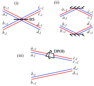
Figure 1: Transformation of OAM modes when they pass through (i) a beam splitter, (ii) a pair of mirrors, and (iii) a Dove prism.

Next, we summarize the transformation properties of OAM modes when they pass through either a beam splitter(BS), a pair of mirrors or a Dove prism. We note that upon reflection an OAM mode changes the sign of its mode index and also picks up an additional phase. This additional phase is equal to $\pi/2$ when the mode reflects from a symmetric beam splitter and is equal to $\pi$ when it reflects from a mirror gonzalez2006optexp . The beam splitter transformation matrix is calculated in the following way. As shown in Fig. 1(i), let us suppose that $a$ and $b$ are the input modes to a beam splitter and $c$ and $d$ are the output modes. The annihilation operators corresponding to mode $a$ are $\hat{a}_{+l}$ and $\hat{a}_{-l}$, etc. Using the standard beam-splitter operator algebra mandel&wolf , we obtain the relationship between the input and output mode annihilation operators and represent it as the matrix equality:

$$\left(\begin{array}[]{c}\hat{c}_{+l}\\ \hat{c}_{-l}\\ \hat{d}_{+l}\\ \hat{d}_{-l}\\ \end{array}\right)=\frac{1}{\sqrt{2}}\left(\begin{array}[]{cccc}0&i&1&0\\ i&0&0&1\\ 1&0&0&i\\ 0&1&i&0\\ \end{array}\right)\left(\begin{array}[]{c}\hat{a}_{+l}\\ \hat{a}_{-l}\\ \hat{b}_{+l}\\ \hat{b}_{-l}\\ \end{array}\right)=M_{\rm bs}\left(\begin{array}[]{c}\hat{a}_{+l}\\ \hat{a}_{-l}\\ \hat{b}_{+l}\\ \hat{b}_{-l}\\ \end{array}\right).$$ (30)

Here the unitary matrix $M_{\rm bs}$ is the beam splitter transformation matrix for OAM modes. In a similar manner, the transformation matrix $M_{\rm mir}$ related to the reflections of two incident modes $a$ and $b$ into the reflected mode $c$ and $d$ [Fig. 1(ii)] can be shown to be

$$M_{\rm mir}=\left(\begin{array}[]{cccc}0&-1&0&0\\ -1&0&0&0\\ 0&0&0&-1\\ 0&0&-1&0\\ \end{array}\right).$$ (35)

Finally, in situations in which one of the modes passes through a Dove prism [Fig. 1(iii)], rotated at an angle $\theta$, the transformation matrix $M_{\rm dp}$ is given by

$$M_{\rm dp}(\theta)=\left(\begin{array}[]{cccc}0&-e^{2il\theta}&0&0\\ -e^{-2il\theta}&0&0&0\\ 0&0&1&0\\ 0&0&0&1\\ \end{array}\right).$$ (40)

The two non-zero off-diagonal matrix elements show that, upon passage through a Dove prism, an OAM mode picks up an additional phase of $\pi-2l\theta$ gonzalez2006optexp , where $l$ is the orbital angular momentum mode index and $\theta$ is the angle of rotation of the Dove prism. The first two diagonal elements are zero due to the fact that upon passage through a Dove prism a modes changes the sign of its OAM mode index. We note that both $M_{\rm mir}$ and $M_{\rm bs}$ are unitary matrices.

We are now ready to analyze the situations shown in Figs. 2 and 3. In these schemes, the entangled photons produced by PDC in modes $s$ and $i$ are mixed at a beam splitter (BS1). A $\theta$ rotation of the Dove prism (DP) then rotates the photon-field in mode $g$ with respect to the field in mode $h$. The photons are then mixed at the second beam splitter (BS2) and detected subsequently in modes $a$ and $b$. Our aim is to determine the resolution and sensitivity with which the rotation angle $\theta$ can be measured. Using the transformation properties of OAM modes as given by Eqs. (30), (35) and (40), we express the output mode annihilation operators in terms of the input mode annihilation operators as

$$O =M_{\rm bs}M_{\rm dp}(\theta)M_{\rm mir}M_{\rm bs}M_{\rm mir}I=MI,$$ (41)

where

$$O=\left(\begin{array}[]{c}\hat{a}_{+l}\\ \hat{a}_{-l}\\ \hat{b}_{+l}\\ \hat{b}_{-l}\\ \end{array}\right)\quad{\rm and}\quad I=\left(\begin{array}[]{c}\hat{s}_{+l}\\ \hat{s}_{-l}\\ \hat{i}_{+l}\\ \hat{i}_{-l}\\ \end{array}\right).$$ (50)

In order to calculate the state in the output modes $a$ and $b$, we need to obtain the inverse relationship, that is, we need to express the input mode annihilation operators in terms of the output mode annihilation operators. Therefore, we invert the above matrix equation and write it as

$$I=M^{-1}O=M^{\dagger}O,$$ (51)

where the last equality results from the fact that $M$ is a unitary matrix $(M^{-1}=M^{\dagger})$, with $|{\rm det}M|=1$, where det denotes the determinant. Now taking the transpose of the above equation we obtain:

$$I^{\dagger}=O^{\dagger}M.$$ (52)

We note that $I^{\dagger}$ and $O^{\dagger}$ are four-element row vectors: $I^{\dagger}=(\hat{s}^{\dagger}_{+l},\hat{s}^{\dagger}_{-l},\hat{i}^{\dagger}_{+l},\hat{i}^{\dagger}_{-l})$ and $O^{\dagger}=(\hat{a}^{\dagger}_{+l},\hat{a}^{\dagger}_{-l},\hat{b}^{\dagger}_{+l},\hat{b}^{\dagger}_{-l})$. Using Eqs. (30) through (41), we solve Eq. (52) to obtain the following operator relations:

$$\hat{s}_{+}^{\dagger}=k_{1}\hat{a}_{+}^{\dagger}+ik_{2}b_{-}^{\dagger},\qquad\hat{s}_{-}^{\dagger}=k_{1}\hat{a}_{-}^{\dagger}+ik_{2}b_{+}^{\dagger};$$ (53a)

$$\hat{i}_{+}^{\dagger}=ik_{4}\hat{a}_{-}^{\dagger}+k_{3}b_{+}^{\dagger},\qquad\hat{i}_{-}^{\dagger}=ik_{4}\hat{a}_{+}^{\dagger}+k_{3}b_{-}^{\dagger};$$ (53b)

where $k_{1}=k_{3}^{*}=\frac{1}{2}(-1-e^{2il\theta})$, $k_{2}=k_{4}^{*}=\frac{1}{2}(-1+e^{2il\theta})$. With the above operator relations, we next calculate the angular resolution and sensitivity that can be obtained with two and four entangled photons.

III.1 Supersensitive measurement with two entangled photons

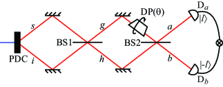
Figure 2: Scheme for supersensitive measurement of angular displacement using two entangled photons. $\theta$ is the angle of rotation of the Dove prism in mode $g$. $D_{a}$ and $D_{b}$ are detectors set to detect one photon each in the mode characterized by index $l$ and $-l$, respectively

.

In this subsection, we illustrate supersensitive angular-displacement measurements with two entangled photons using the detection scheme depicted in Fig. 2. We consider a class of states $|\psi_{2}^{l}\rangle$ that are obtained from Eq. (10) by keeping only terms with the OAM mode indices $\pm l$ for a given value of $l$:

$$|\psi_{2}^{l}\rangle=\sqrt{\frac{1}{2}}\left[|1\rangle_{s_{+l}}|1\rangle_{i_{-l}}+|1\rangle_{s_{-l}}|1\rangle_{i_{+l}}\right].$$ (54)

In practice, such states can be obtained from the state produced by PDC by placing appropriate phase apertures in the paths of the signal and idler photons leach2009optexp . We note that we have used the alternative notation in writing the state $|\psi_{2}^{l}\rangle$, which can be written in terms of the input mode creation operators as

$$|\psi_{2}^{l}\rangle=\sqrt{\frac{1}{2}}\left[\hat{s}^{\dagger}_{+l}\hat{i}^{\dagger}_{-l}+\hat{s}^{\dagger}_{-l}\hat{i}^{\dagger}_{+l}\right]|{\rm vac}\rangle.$$ (55)

Using the operator relations of Eq. (53), we express the above state in terms of the output mode creation operators to obtain

$$|\psi_{2}^{l}\rangle=\sqrt{\frac{1}{2}}[(k_{1}\hat{a}_{+l}^{\dagger}+ik_{2}b_{-l}^{\dagger})(ik_{4}\hat{a}_{+l}^{\dagger}+k_{3}b_{-l}^{\dagger})\\ +(k_{1}\hat{a}_{-l}^{\dagger}+ik_{2}b_{+l}^{\dagger})(ik_{4}\hat{a}_{-l}^{\dagger}+k_{3}b_{+l}^{\dagger})]|{\rm vac}\rangle.$$ (56)

We now estimate the angular resolution and sensitivity through use of the following measurement operator kolkiran2007optexp :

$$\hat{A}_{2}=|1\rangle_{a_{+l}}|1\rangle_{b_{-l}}{}_{a_{+l}}\langle 1|{}_{b_{-l}}\langle-1|,$$ (57)

which measures the probability of detecting a photon in mode $a$ with the OAM mode index $l$ and another photon in mode $b$ with the OAM mode index $-l$. The measurement operator $A_{2}$ does not see the complete state $|\psi_{2}^{l}\rangle$; the effective post-selected state $|\psi_{2}^{l}\rangle_{\rm post}$ that $\hat{A}_{2}$ sees is obtained from $|\psi_{2}^{l}\rangle$ by keeping only the terms containing $\hat{a}_{+l}^{\dagger}\hat{b}_{-l}^{\dagger}$. $|\psi_{2}^{l}\rangle_{\rm post}$ is given by:

$$|\psi_{2}^{l}\rangle_{\rm post} =\frac{1}{\sqrt{2}}(k_{1}^{2}-k_{2}^{2})\hat{a}_{+l}\hat{b}_{-l}|{\rm vac}\rangle$$

$$=-\frac{1}{2\sqrt{2}}\left[1+e^{4il\theta}\right]|1\rangle_{a_{+l}}|1\rangle_{b_{-l}}.$$ (58)

Taking the inner product of the above state with itself, we obtain ${}_{\rm post}\langle\psi_{2}^{l}|\psi_{2}^{l}\rangle_{\rm post}=\frac{1}{2}\cos^{2}2l\theta$. We note that even in the best case in which $\theta=0$, only half of the input state is detected in modes $a_{+l}$ and $b_{-l}$, since the other half of the state ends up in modes $a_{-l}$ and $b_{+l}$. The expectation value of the measurement operator $\hat{A}_{2}$ is $\langle\hat{A}_{2}\rangle={\rm Tr}[\hat{A}_{2}|\psi_{2}^{l}\rangle\langle\psi_{2}^{l}|]={\rm Tr}[\hat{A}_{2}|\psi_{2}^{l}\rangle_{\rm post}{}_{\rm post}\langle\psi_{2}^{l}|]=\cos^{2}(2l\theta)$. We thus see that there is a two-fold enhancement in the resolution of angular displacement measurements. Next, noting that $\langle\hat{A}_{2}^{2}\rangle=\langle\hat{A}_{2}\rangle=\cos^{2}(2l\theta)$, we obtain

$$\langle\Delta\hat{A}_{2}\rangle=\sqrt{\langle\hat{A}_{2}^{2}\rangle-\langle\hat{A}_{2}\rangle^{2}}=\frac{\sin(4l\theta)}{2}.$$ (59)

Therefore, the uncertainty $\Delta\theta$ in the estimation of the angular displacement is

$$\Delta\theta=\frac{\langle\Delta\hat{A}_{2}\rangle}{|\partial\langle\hat{A}_{2}\rangle\big{/}\partial\theta|}=\frac{1}{4l}.$$ (60)

In the next subsection we calculate the angular resolution and sensitivity using four entangled photons and also with $N$ entangled photons. We then compare these results with the angular resolution and sensitivity obtained with $N$ one-photon Fock state input.

III.2 Angular super-sensitivity with four entangled photons

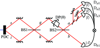
Figure 3: A scheme for supersensitive measurement of angular displacement using four entangled photons. $\theta$ is the angle of rotation of the Dove prism in mode $g$. $D_{a1}$, $D_{a2}$, $D_{a3}$ and $D_{b1}$ are detectors set to detect one photon each in the mode characterized by index $l$, $l$, $l$, and $-l$, respectively.

We now consider the class of four-photon entangled states $|\psi_{4}^{l}\rangle$ that is obtained from Eq. (12) by keeping only terms with OAM mode indices $\pm l$ for a given value of $l$, that is

$$|\psi_{4}^{l}\rangle=\frac{1}{2}\Big{[}|2\rangle_{s_{+l}}|2\rangle_{i_{-l}}+|2\rangle_{s_{-l}}|2\rangle_{i_{+l}}+\\ |1\rangle_{s_{+l}}|1\rangle_{s_{-l}}|1\rangle_{i_{+l}}|1\rangle_{i_{-l}}+|1\rangle_{s_{-l}}|1\rangle_{s_{+l}}|1\rangle_{i_{-l}}|1\rangle_{i_{+l}}\Big{]}.$$ (61)

The state $|\psi_{4}^{l}\rangle$ can be written in terms of the input mode creation operators as

$$|\psi_{4}^{l}\rangle=\frac{1}{2}[\hat{s}^{\dagger}_{+l}\hat{s}^{\dagger}_{+l}\hat{i}^{\dagger}_{-l}\hat{i}^{\dagger}_{-l}+\hat{s}^{\dagger}_{-l}\hat{s}^{\dagger}_{-l}\hat{i}^{\dagger}_{+l}\hat{i}^{\dagger}_{+l}\\ +2\hat{s}^{\dagger}_{+l}\hat{s}^{\dagger}_{-l}\hat{i}^{\dagger}_{-l}\hat{i}^{\dagger}_{+l}]|{\rm vac}\rangle.$$ (62)

Our four-photon measurement operator $\hat{A}_{4}$ is

$$\hat{A}_{4}=|3\rangle_{a_{+l}}|1\rangle_{b_{-l}}{}_{a_{+l}}\langle 3|{}_{b_{-l}}\langle 1|,$$ (63)

which measures the probability of detecting three photons in mode $a_{+l}$ and one photon in mode $b_{-l}$. In Fig. 3, we have depicted one possible way of carrying out such a measurement kolkiran2007optexp . The particular choice of the measurement operator is motivated by the fact that in order to achieve super-sensitivity, the four-photon measurement needs to post-select the ensemble that consists only of the maximally entangled four-photon states. The effective post-selected state $|\psi_{4}^{l}\rangle_{\rm post}$ that the measurement operator $\hat{A}_{4}$ sees is obtained by first expressing the state $|\psi_{4}^{l}\rangle$ in terms of the output state creation operators using the operator relations given in Eq. (53) and then keeping only the terms containing $\hat{a}^{\dagger}_{+l}\hat{a}^{\dagger}_{+l}\hat{a}^{\dagger}_{+l}\hat{b}^{\dagger}_{-l}$ in the expansion. After a straightforward calculation we obtain:

$$|\psi_{4}^{l}\rangle_{\rm post} =\frac{1}{4}(-2ik_{1}^{3}k_{2}-2ik_{1}k_{2}^{3})\hat{a}^{\dagger}_{+l}\hat{a}^{\dagger}_{+l}\hat{a}^{\dagger}_{+l}\hat{b}^{\dagger}_{-l}|{\rm vac}\rangle$$

$$=\frac{-i\sqrt{6}}{16}\left(1-e^{8il\theta}\right)|3\rangle_{a_{+l}}|1\rangle_{b_{-l}}.$$ (64)

Now taking the inner product of the state with itself, we find ${}_{\rm post}\langle\psi_{4}^{l}|\psi_{4}^{l}\rangle_{\rm post}=\frac{3}{32}\sin^{2}4l\theta$. We note that even in the best case, when $4l\theta=\pi/2$, only 3/32nd of the input intensity is detected by the measurement operator. The expectation value of the measurement operator is $\langle\hat{A}_{4}\rangle=\langle\hat{A}_{4}^{2}\rangle={\rm Tr}[\hat{A}_{4}|\psi_{4}^{l}\rangle\langle\psi_{4}^{l}|]={\rm Tr}[\hat{A}_{4}|\psi_{4}^{l}\rangle_{\rm post}{}_{\rm post}\langle\psi_{4}^{l}|]=\sin^{2}(4l\theta)$, thus showing a four-fold enhancement in angular resolution. The uncertainty $\langle\Delta\hat{A}_{4}\rangle$ is given by $\langle\Delta\hat{A}_{4}\rangle=\sqrt{\langle\hat{A}_{4}\rangle-\langle\hat{A}_{4}\rangle^{2}}=\sin(8l\theta)/2$. Therefore, for the uncertainty $\Delta\theta$ in the estimation of angular displacement, we obtain

$$\Delta\theta=\frac{\langle\Delta\hat{A}_{4}\rangle}{|\partial\langle\hat{A}_{4}\rangle\big{/}\partial\theta|}=\frac{1}{8l}.$$ (65)

III.3 Angular super-sensitivity with $N$ entangled photons

Proceeding in the same manner, one can show that, with $N$ entangled photons and a suitable detection scheme, the angular resolution gets enhanced by a factor of $N$ and the angular sensitivity improves as

$$\Delta\theta=\frac{1}{2Nl}.$$ (66)

We note that the angular sensitivity obtained with $N$ entangled photons is greater than the angular sensitivity $\Delta\theta_{\rm Fock}$ obtained with a stream of $N$ one-photon Fock state input to an interferometer, which can be shown to be $\Delta\theta_{\rm Fock}=1/(2\sqrt{N}l)$ scully1993pra . We further note that Eq. (66) is the maximum angular sensitivity that can be obtained with $N$ entangled photons. In deriving Eq. (66), we have not included other factors, such as the effects due to post-selection, that also affect the sensitivity in a laboratory situation. Some of these factors have been discussed by Okamoto et al. okamoto2008njp in their work on phase super-sensitivity.

IV Conclusions

In conclusion, we have shown that the use of entangled photons having non-zero orbital angular momentum increases the resolution and sensitivity of angular-displacement measurements performed using an interferometer. Using a $4\times 4$ matrix formulation to study the propagation of entangled OAM modes, we have explicitly analyzed measurement schemes for two and four entangled photons. We have found that the resolution of angular-displacement measurements scales as $Nl$ while the angular sensitivity increases as $1/(2Nl)$, where $N$ is the number of entangled photons and $l$ the magnitude of the orbital-angular-momentum mode index. It has previously been established mair2001nature ; leach2010science that the orbital angular momentum of light constitutes a useful degree of freedom for applications in quantum optics and quantum information science. The work presented here provides another such example. The ability to detect small rotations of optical components or of light beams themselves holds promise for many applications both in remote sensing and for performing fundamental studies of the propagation of light through optical materials.

References

- (1) M. Scully and M. Zubairy, Quantum Optics (Cambridge Univ Press, Cambridge, UK, 1997).
- (2) H. Lee, P. Kok, and J. Dowling, Journal of Modern Optics 49, 2325 (2002).
- (3) C. Caves, Physical Review D 23, 1693 (1981).
- (4) B. Yurke, Physical review letters 56, 1515 (1986).
- (5) A. N. Boto, P. Kok, D. S. Abrams, S. L. Braunstein, C. P. Williams, and J. P. Dowling, Phys. Rev. Lett. 85, 2733 (2000).
- (6) M. D’Angelo, M. V. Chekhova, and Y. Shih, Phys. Rev. Lett. 87, 013602 (2001).
- (7) P. Walther, J. Pan, M. Aspelmeyer, R. Ursin, S. Gasparoni, and A. Zeilinger, Nature 429, 158 (2004).
- (8) M. Mitchell, J. Lundeen, and A. Steinberg, Nature 429, 161 (2004).
- (9) A. Kolkiran and G. S. Agarwal, Opt. Express 15, 6798 (2007).
- (10) F. Sun, Z. Ou, and G. Guo, Physical Review A 73, 23808 (2006).
- (11) T. Nagata, R. Okamoto, J. L. O’Brien, K. Sasaki, and S. Takeuchi, Science 316, 726 (2007).
- (12) K. Resch, K. Pregnell, R. Prevedel, A. Gilchrist, G. Pryde, J. O brien, and A. White, Physical review letters 98, 223601 (2007).
- (13) Z. Y. Ou, L. J. Wang, and L. Mandel, Phys. Rev. A 40, 1428 (1989).
- (14) L. Allen, M. Beijersbergen, R. Spreeuw, and J. Woerdman, Phys. Rev. A 45, 8185 (1992).
- (15) C. K. Law and J. H. Eberly, Phys. Rev. Lett. 92, 127903 (2004).
- (16) N. González, G. Molina-Terriza, and J. P. Torres, Opt. Express 14, 9093 (2006).
- (17) L. Mandel and E. Wolf, Optical Coherence and Quantum Optics (Cambridge university press, New York, 1995).
- (18) J. Leach, B. Jack, J. Romero, M. Ritsch-Marte, R. W. Boyd, A. K. Jha, S. M. Barnett, S. Franke-Arnold, and M. J. Padgett, Opt. Express 17, 8287 (2009).
- (19) M. O. Scully and J. P. Dowling, Phys. Rev. A 48, 3186 (1993).
- (20) R. Okamoto, H. Hofmann, T. Nagata, J. O’Brien, K. Sasaki, and S. Takeuchi, New Journal of Physics 10, 073033 (2008).
- (21) A. Mair, A. Vaziri, G. Weihs, and A. Zeilinger, Nature 412, 313 (2001).
- (22) J. Leach, B. Jack, J. Romero, A. Jha, A. Yao, S. Franke-Arnold, D. Ireland, R. Boyd, S. Barnett, and M. Padgett, Science 329, 662 (2010).