Spin-dependent Scattering by a Potential Barrier on a Nanotube

Abstract

The electron spin effects on the surface of a nanotube have been considered through the spin-orbit interaction (SOI), arising from the electron confinement on the surface of the nanotube. This is of the same nature as the Rashba-Bychkov SOI at a semiconductor heterojunction. We estimate the effect of disorder within a potential barrier on the transmission probability. Using a continuum model, we obtained analytic expressions for the spin-split energy bands for electrons on the surface of nanotubes in the presence of SOI. First we calculate analytically the scattering amplitudes from a potential barrier located around the axis of the nanotube into spin-dependent states. The effect of disorder on the scattering process is included phenomenologically and induces a reduction in the transition probability. We analyzed the relative role of SOI and disorder on the transmission probability which depends on the angular and linear momentum of the incoming particle, and its spin orientation. We demonstrated that in the presence of disorder perfect transmission may not be achieved for finite barrier heights.

I Introduction

Carbon nanotubes which are members of the fullerene family, have novel properties that make them potentially useful in many applications in electronics, optics, and other fields of nanotechnology and materials science. Their strength is extraordinary, they possess unique electrical properties, and are efficient thermal conductors. The nanotube diameter is on the order of a few nanometers and the nanotube length several millimeters. Nanotube ends might be capped with a hemisphere of the buckyball structure or some other material providing a potential barrier for the carrier electrons on the nanotube. Furthermore, there may be a coupling between a particle’s intrinsic (spin) and its extrinsic (orbital motion) degrees of freedom, thereby giving rise to a spin-orbit interaction (SOI) term in the Hamiltonian describing the energy eigenstates of the nanotube. The SOI may be due to the electromagnetic interaction between the electron’s spin and the nucleus’ electric field through which the electron moves.nitta As a matter of fact, the SOI on the nanotube is of the same type as the Rashba SOI at a hetrojunction of two types of semiconductors which has given rise to many interesting properties such as spontaneous spin effects in a two-dimensional electron gas (2DEG).gumbs

Detailed theoretical studies of the spin-orbit coupling in graphene and carbon nanotubes have been carried out recently.DeMartino+Egger ; guinea ; kane ; prb1 This work was done in conjunction with recent experiments which have shown that a gate voltage applied perpendicular to the axis of a carbon nanotube can cause an observable SOI.9a ; 9 ; 10 These studies were stimulated by the consequences of the presence of SOI on transport properties in carbon nanotubes. The origin of SOI is that, when electrons moving in an electrostatic potential $\Phi({\bf r})$ (due to ions or gate fields) experience an effective magnetic field, ${\bf B}_{eff}\propto{\bf v}\times\nabla\Phi$ in their rest. For graphene, intrinsic SOI comes from next-neighbor interactions and is therefore small ($\sim\ 10$ mK= $10^{-3}$ meV). guinea ; prb1 However, nearest-neighbor terms are nonzero when external (Rashba) electric fields or curvature-induced overlap changes break the symmetry which is responsible for the vanishing of the nearest-neighbor hopping. Therefore, dominant SOI in the absence of external fields is naturally present in carbon nanotubes. For nanotubes, the Rashba field gives a small effect since it is averaged over the circumference. DeMartino+Egger ; guinea ; kane ; prb1 However, when electrostatic gates are applied to carbon nanotubes, and in the vicinity of a van Hove singularity,yonatan the Rashba SOI is enhanced and could lead to observable effects.

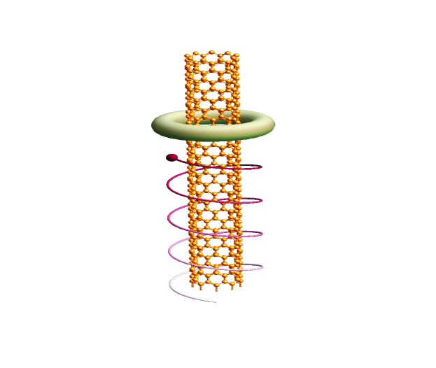
Figure 1: (Color online) Schematic illustration of the nanotube in the presence of a particle having linear momentum parallel to the axis of the nanotube as well as angular momentum around its axis. The incoming particle impinges on a barrier of uniform thickness.

We will assume that the nanotube we are dealing with is of high quality but will investigate the role played by disorder within the potential barrier on the electron transport. The electron eigenstates are labeled by quantum numbers representing its two degrees of freedom.yonatan ; yonatan2 These are the wave number $k_{z}$ along the axis of the nanotube and the angular momentum quantum number $l$ around its axis. The SOI shifts and splits the energy levels giving eigenstates which may be interpreted as a superposition of the $|\uparrow\rangle$ and $|\downarrow\rangle$ spin states. With this background information, we are motivated to consider a problem involving spin currentsspincurrent along the surface of a nanotube and the associated transmission and reflection probabilities from a potential barrier. The potential barrier may be produced by an electrostatic gate voltage, whose electric field has the ability to act as an extra control parameter to exclude electrons from a region of the nanotube, thereby producing a potential barrier. Multiple gates (three top gates and a back gate) have been reported to be deposited on the surface of carbon nanotubes to produce quantum dots.marcus Sharmascience has reviewed a method for generating spin currents and discusses ways in which to overcome some obstacles. There have been several recent papers dealing with the penetration of spin-currents through a potential barrier in a 2DEG. sablikov ; tkach ; sukhanov ; sablikov2 In this regard, we consider an electron with linear wave number $k_{z}^{i}$ and angular momentum quantum number $L^{i}$ having probability amplitude $a_{+}$ in the $|\uparrow\rangle$ state and probability amplitude $a_{-}$ in the $|\downarrow\rangle$ state. The electron is incident on a cylindrical potential barrier, as shown in Fig. 1. We consider the effect of disorder arising from impurities, defects, or by the atoms/molecules composing the nanotube which simply oscillate around their equilibrium positions has on the scattering process. We first calculate the tunneling and reflection probabilities in the absence of disorder. In principle, these calculations require a knowledge of the electron eigenstates in the presence of SOI. For the ballistic transport, we assume that the electron mean free path is much longer than the diameter of the nanotube so that the electron’s motion is only altered by interaction with the potential barrier. We then outline and employ a phenomenological theory to analyze the effect due to disorder on the tunneling.

The outline of the remainder of this paper is as follows. In Section II, we present the model spin-orbit Hamiltonian for single electrons and the corresponding single-particle eigenstates for an intercalated carbon nanotube. Section III is devoted to calculating the transmission and reflection probability amplitudes through a cylindrical potential barrier encircling the axis of the nanotube in the absence of disorder. In Sec. IV, we introduce and discuss procedures for including the effect of disorder on the tunneling probability through the potential barrier. We present and discuss our numerical calculations in Section   V. Some concluding remarks are given in Section VI.

II The Model Spin-Orbit Hamiltonian

Let us consider a nanotube with its axis along the $z$-axis in the presence of SO coupling. The Hamiltonian for an electron with momentum ${\bf p}$ on the surface of a cylinder takes the following form yonatan ; yonatan2

$$H=\frac{1}{2m^{\ast}}\left(\hat{p}^{2}_{z}+\hat{p}^{2}_{\phi}\right)+\frac{\alpha_{R}}{\hbar}\left[(\sigma_{1}\sin\phi-\sigma_{2}\cos\phi)\hat{p}_{z}+\sigma_{3}\hat{p}_{\phi}\right]\ ,$$ (1)

where $\alpha_{R}$ is the Rashba SOI parameter due to radial confinement and $\sigma_{i}$ are the Pauli matrices. The general solutions are yonatan

$$|u_{\nu}(\phi,z)\rangle = \left(\begin{array}[]{ccc}u^{+}_{\nu}(\phi,z)&\\ u^{-}_{\nu}(\phi,z)&\end{array}\right)$$ (4)

$$u^{(\pm)}_{\nu}(\phi,z) = \frac{e^{ikz}}{\sqrt{L_{z}}}\Phi^{(\pm)}(\phi),\;\;\;\;\Phi^{(\pm)}(\phi)=\frac{1}{\sqrt{2\pi}}\sum^{\infty}_{l=-\infty}c^{(\pm)}_{l}(k_{z})e^{il\phi}\ .$$ (5)

The eigenenergies which depend on $k_{z}$, $l$ and $\alpha_{R}$ are given by

$${\cal E}^{s}(k_{z},l,\alpha_{R}) = \frac{1}{2}\left[E^{2}_{l+1}(k_{z},\alpha_{R})+E^{1}_{l}(k_{z},\alpha_{R})\right]+\frac{s}{2}\sqrt{\left[E^{2}_{l+1}(k_{z},\alpha_{R})-E^{1}_{l}(k_{z},\alpha_{R})\right]^{2}+4\alpha^{2}_{R}k^{2}_{z}}\ ,$$ (6)

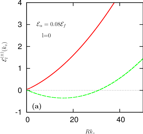
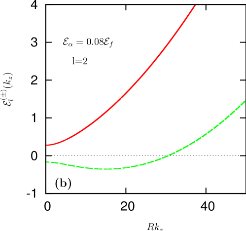
Figure 2: (Color online) Energy eigenvalues as a function of $k_{z}$ in the presence of SOI ${\cal E}_{\alpha}$. In (a) $l=0$ and (b) $l=2$ for the angular momentum quantum number. The continuous line is for “$+$” state while the dashed line is for “$-$” state. $R=10$nm is the radius of the nanotube. For $l\neq 0$ ((b) $l=2$) there is always an energy gap at $k_{z}=0$.

where $E^{1}_{l}(k_{z},\alpha_{R})=E^{(0)}(k_{z},l)-\frac{\alpha_{R}l}{R}=E^{(0)}(k_{z},l)-l{\cal E}_{\alpha}$ and $E^{2}_{l}(k_{z},\alpha_{R})=E^{(0)}(k_{z},l)+\frac{\alpha_{R}l}{R}=E^{(0)}(k_{z},l)+l{\cal E}_{\alpha}$ with $E^{(0)}(k_{z},l)=\frac{\hbar^{2}k^{2}_{z}}{2m^{\ast}}+\frac{\hbar^{2}l^{2}}{2m^{\ast}R^{2}}=\frac{\hbar^{2}k^{2}_{z}}{2m^{\ast}}+l^{2}{\cal E}_{R}$. Here, $s=\pm$ denotes the two pseudospin orientations. Figures (2a) and (2b) depict the dispersion relation given in Eq. (6) exhibiting the split between the $``+"$ and $``-"$ states. In these plots, we chose the angular momentum quantum number $l=0$ and $l=2$. At $k_{z}=0$, the gap in the spectrum is determined by the SOI as well as the radius of the nanotube. The corresponding eigenspinors are

$$|\psi_{k_{z},L,s}(z,\phi)\rangle=\left(\begin{array}[]{ccc}u^{+}(\phi,z)&\\ u^{-}(\phi,z)&\end{array}\right)^{s}_{k_{z},L} = \frac{c^{s}_{L}(k_{z},\alpha_{R})}{\sqrt{2\pi L_{z}}}\left(\begin{array}[]{ccc}1&\\ \chi^{s}_{L}(k_{z},\alpha_{R})&\end{array}\right)e^{i(k_{z}z+L\phi)}\ ,$$ (11)

where

$$\chi^{s}_{L}(k_{z},\alpha_{R})=e^{i\phi}[E^{1}_{L}(k_{z},\alpha_{R})-{\cal E}^{s}(k_{z},L,\alpha_{R})]/ik_{z}\alpha_{R}.$$

Orthonormality $\langle\psi_{k_{z},L^{\prime},s^{\prime}}(z,\phi)|\psi_{k_{z},L,s}(z,\phi)\rangle=\delta_{LL^{\prime}}\delta_{ss^{\prime}}$ yields

$$c^{s}_{L}(k_{z},\alpha_{R}) = [1+\chi^{s}_{L}(k_{z},\alpha_{R})\chi^{s\ \ast}_{L}(k_{z},\alpha_{R})]^{-1/2}$$

$$= k_{z}\alpha_{R}[(E^{1}_{L}(k_{z},\alpha_{R})-{\cal E}^{s}(k_{z},L,\alpha_{R}))^{2}+\alpha^{2}_{R}k^{2}_{z}]^{-1/2}$$

$$\chi^{-}_{L}(k_{z},\alpha_{R}) = \frac{-1}{\chi^{+\ \ast}_{L}(k_{z},\alpha_{R})}\ .$$ (12)

II.1 Presence of a Barrier

In the presence of a potential barrier of height $U$ and width $w$, as shown in Fig. 1, the energies and eigenspinors within the barrier are obtained in a similar fashion as in the absence of a barrier. The effect of the barrier is to shift energy eigenvalues as follows,

$${\cal E}^{s}(k^{b}_{z},l,\alpha_{R}) \to {\cal E}^{s}(k^{b}_{z},l,\alpha_{R})-U=\bar{\cal E}^{s}(k^{b}_{z},l,\alpha_{R})$$ (13)

$$= \frac{1}{2}\left[E^{2}_{l+1}(k^{b}_{z},\alpha_{R})+E^{1}_{l}(k^{b}_{z},\alpha_{R})\right]+\frac{s}{2}\sqrt{\left[E^{2}_{l+1}(k^{b}_{z},\alpha_{R})-E^{1}_{l}(k^{b}_{z},\alpha_{R})\right]^{2}+4\alpha^{2}_{R}(k^{b}_{z})^{2}}.$$

Outside the barrier ($U=0$), we consider only states with $k_{z}^{2}\geq 0$ and we have $e^{\pm ik_{z}}$ type solutions. Inside the barrier for small enough barrier heights Eq. (13)implies $(k^{b}_{z})^{2}\geq 0$ and we still have $e^{\pm ik^{b}_{z}z}$ type solutions. However as the height of the barrier increases Eq. 13 cannot be satisfied with real $k^{b}_{z}$. In this case, we seek a solution with $k^{b}_{z}\to\pm i\kappa_{z}$ inside the barrier region giving $e^{\pm\kappa_{z}z}$ dependence exhibiting decay or growth.

We note that for real $k^{b}_{z}$, $\bar{\cal E}^{+}(k^{b}_{z},l,\alpha_{R})$ is a monotonically increasing even function of $k^{b}_{z}$, with a minimum at $k^{+}_{min}=0$ given by $\bar{\cal E}^{+}(0,l,\alpha_{R})=E^{2}_{l+1}(0,\alpha_{R})>0$, while $\bar{\cal E}^{-}(k^{b}_{z},l,\alpha_{R})$ attains a local maximum at $k^{-}_{max}=0$ given by $E^{1}_{l}(0,\alpha_{R})=l^{2}{\cal E}_{R}-l{\cal E}_{\alpha}$ and can be negative for high enough ${\cal E}_{\alpha}$. Consequently, we have a finite difference in energy between the $``+"$ and the $``-"$ states at $k^{b}_{z}=0$. For nanotubes with large radius ($R\to\infty$), both ${\cal E}_{R}$ and ${\cal E}_{\alpha}$ go to zero and the energy difference between the states vanishes at $k^{b}_{z}=0$. For real $k^{b}_{z}$, $\bar{\cal E}^{-}(k^{b}_{z},l)$ attains a minima at

$$k^{-}_{min}R=\pm\left[\left(\frac{{\cal E}_{\alpha}}{{\cal E}_{R}}\right)^{2}-(2l+1)^{2}\left(1+\frac{{\cal E}_{\alpha}}{{\cal E}_{R}}\right)\right]^{1/2},$$

given by $\bar{\cal E}^{-}(k^{-}_{min},l,\alpha_{R})<0$. However, for high enough potential $U$, $\bar{\cal E}^{\pm}(k^{b}_{z},l,\alpha_{R})$ in Eq.  (13) can have values less than $\bar{\cal E}^{\pm}(k^{\pm}_{min},l,\alpha_{R})$ and $k^{b}_{z}$ becomes imaginary, $k^{b}_{z}\to\pm i\kappa_{z}$ and the state exhibit $e^{\pm\kappa_{z}z}$ dependence within the barrier. The derivation in this case is the same as the derivation for the energy eigenvalues and eigenspinors. The eigenenergies are given by,

$${\cal E}^{s}(\kappa_{z},l,\alpha_{R})-U = \frac{1}{2}\left[E^{2}_{l+1}(\kappa_{z},\alpha_{R})+E^{1}_{l}(\kappa_{z},\alpha_{R})\right]+\frac{s}{2}\sqrt{\left[E^{2}_{l+1}(\kappa_{z},\alpha_{R})-E^{1}_{l}(\kappa_{z},\alpha_{R})\right]^{2}-4\alpha^{2}_{R}\kappa^{2}_{z}}\ ,$$ (14)

where $E^{1}_{l}(\kappa_{z},\alpha_{R})=E^{(0)}(\kappa_{z},l)-\frac{\alpha_{R}l}{R}$ and $E^{2}_{l}(\kappa_{z},\alpha_{R})=E^{(0)}(\kappa_{z},l)+\frac{\alpha_{R}l}{R}$, with $E^{(0)}(\kappa_{z},l)=\frac{-\hbar^{2}\kappa^{2}_{z}}{2m^{\ast}}+\frac{\hbar^{2}l^{2}}{2m^{*}R^{2}}$. The eigenspinors are similarly modified with $k_{z}\to\pm i\kappa$.

II.2 Limiting case $R\to\infty$

We show here that the results in the previous section reduce to the familiar results of 2 DEG with SOI in the limit $R\to\infty$. For $R\to\infty$, $l/R\to k_{\perp}$ and $l\phi=(l/R)R\phi\to k_{\perp}x_{\perp}$, we obtain for the eigenvalues

$$\lim_{R\to\infty}{\cal E}^{s}(k_{z},l) \to E^{0}(k_{z},l)+s\alpha_{R}\sqrt{k_{\perp}^{2}+k_{z}^{2}}$$ (15)

$$= E^{0}(k_{z},l)+s\alpha_{R}k.$$

By making use of

$$\lim_{R\to\infty}\chi^{s}_{L}(k_{z},\alpha_{R}) \to \frac{i(k_{\perp}+sk)}{k_{z}}$$ (16)

$$\lim_{R\to\infty}c^{s}(k_{z},L) \to \frac{k_{z}}{\left[k^{2}_{z}+(k_{\perp}+sk)^{2})\right]^{1/2}}\ ,$$ (17)

the normalized eigenspinors become

$$|\psi^{+}(z,x_{\perp})\rangle=\frac{k_{z}}{\sqrt{k_{z}^{2}+(k_{\perp}+k)^{2}}}\left(\begin{array}[]{ccc}1&\\ \frac{i(k_{\perp}+k)}{k_{z}}&\end{array}\right)\frac{e^{i(k_{z}z+k_{\perp}x_{\perp})}}{\sqrt{A}}$$ (20)

$$|\psi^{-}(z,x_{\perp})\rangle=\frac{k_{z}}{\sqrt{k_{z}^{2}+(k_{\perp}-k)^{2}}}\left(\begin{array}[]{ccc}1\\ \frac{i(k_{\perp}-k)}{k_{z}}&\end{array}\right)\frac{e^{i(k_{z}z+k_{\perp}x_{\perp})}}{\sqrt{A}}\ ,$$ (23)

where $A=2\pi RL_{z}$, where $L_{z}$ is a normalization length. At first glance, these expressions look different from the 2DEG expressions for the eigenspinors. The reason for this is that the geometry used here is different (rotated). It can be shown that if we start with a different geometry for the 2DEG confinement we obtain the above result. Here, in the limit $R\to\infty$, we have a confinement in the $y-z$ plane and the SO Hamiltonian for the 2DEG is written as

$$H_{SO} = \frac{\hbar}{(2m^{\ast}c)^{2}}{\bf\nabla}V_{x}\cdot(\mbox{\boldmath$\sigma$}\times{\bf p})_{x}$$ (24)

$$= i\alpha\left(\sigma_{3}\frac{\partial}{\partial y}-\sigma_{2}\frac{\partial}{\partial z}\right)\ .$$

This leads to the following eigenvalue problem

$$\left(\matrix{E^{(0)}-\alpha k_{y}&-ik_{z}\alpha\cr ik_{z}\alpha&E^{(0)}+\alpha k_{y}\cr}\right)\left(\matrix{c^{+}\cr c^{-}\cr}\right)={\cal E}\left(\matrix{c^{+}\cr c^{-}\cr}\right)\ .$$ (25)

Here, $E^{(0)}=\frac{\hbar^{2}}{2m^{\ast}}(k_{y}^{2}+k_{z}^{2})=\frac{\hbar^{2}k^{2}}{2m^{\ast}}$, and the eigenvalue equation is given by

$$\left((E^{(0)}-{\cal E})-\alpha k_{y}\right)\left((E^{(0)}-{\cal E})+\alpha k_{y}\right)-\alpha^{2}k_{z}^{2}=0$$

$$({\cal E}-E^{(0)})^{2}-\alpha^{2}(k_{y}^{2}+k_{z}^{2})=0$$

$${\cal E}^{s}=E^{(0)}+s\alpha k\ .$$ (26)

The eigenspinors are given by

$${\cal E}^{+}:\;\;\;\;\; (E^{(0)}-\alpha k_{y})c^{+}-i\alpha k_{z}c^{-}={\cal E}^{+}c^{+}$$

$$c^{-}=({\cal E}^{+}-E^{(0)}+\alpha k_{y})\frac{c^{+}}{-i\alpha k_{z}}=\frac{i(k_{y}+k)}{k_{z}}c^{+}$$

$${\cal E}^{-}:\;\;\;\;\; (E^{(0)}+\alpha k_{y})c^{-}+i\alpha k_{z}c^{+}={\cal E}^{-}c^{-}$$ (27)

$$c^{+}=({\cal E}^{-}-E^{(0)}-\alpha k_{y})\frac{c^{-}}{i\alpha k_{z}}=\frac{i(k_{y}-k)}{k_{z}}c^{-}\ .$$

These lead to the eigenspinors obtained above in the limit $R\to\infty$. The difference in appearance is simply to the choice of the direction of confinement and all the eigenspinors are equivalent.

III Tunneling through a Potential Barrier

We consider a potential barrier localized on the nanotube. The potential has height $U$ and width $w$. We calculate the transition probability of an electron propagating in the $+z$-direction. We have three regions of interest. In region I, $z<0$, we consider a specific incoming state (a linear combination of the up and down-spin eigenstates) with wave vector $k^{i}_{z}$ and angular momentum quantum $L^{i}$ as well as the reflected state with wave vector $-k^{i}_{z}$, with two possible spin states. Therefore, in region I, before the barrier, the wavefunction is

$$|\psi^{1}_{k^{i}_{z},L^{i}}\rangle = a_{+}|k^{i}_{z},L^{i},+\rangle+a_{-}|k^{i}_{z},L^{i},-\rangle+\sum_{ss^{\prime}=\pm}r_{ss^{\prime}}|-k^{i}_{z},L^{r},ss^{\prime}\rangle.$$

$$1 = |a_{+}|^{2}+|a_{-}|^{2}\ .$$ (28)

That is, in region I, we have an incoming superposition of $\pm$ eigenspinors which are normalized and a reflected superposition of $\pm$ states. In region III, after the barrier we have only a transmitted state given by

$$|\psi^{3}_{k^{t}_{z},L^{t},s}\rangle=\sum_{ss^{\prime}=\pm}t_{ss^{\prime}}|k^{i}_{z},L^{t},ss^{\prime}\rangle\ .$$ (29)

In region II, inside the barrier, the form of the wavefunction is the same as in Eq. (11) with a different $k_{z}$ due to the presence of the potential barrier and we have

$$|\psi^{2}_{k^{b}_{z},L^{b},s}\rangle=\sum_{rs^{\prime}=\pm}b_{rs^{\prime}}|rk^{b}_{z},L^{b},rs^{\prime}\rangle\ .$$ (30)

Here, $r_{ss^{\prime}}$, $t_{ss^{\prime}}$ and $b_{rr^{\prime}}$ are the matrix elements associated with the scattering process corresponding to reflection, transmission and barrier states. They are determined using the appropriate boundary conditions.

Let us consider the case when the incoming electron is given by a superposition states of Eq. (11). Continuity of $\psi$ at $z=0$ gives

$$\sum_{s=\pm}a_{s}c^{s}_{L^{i}}(k^{i}_{z})\left(\begin{array}[]{ccc}1&\\ \chi^{s}_{L^{i}}(k^{i}_{z})&\end{array}\right)e^{iL^{i}\phi}+\sum_{ss^{\prime}=\pm}r_{-ss^{\prime}}c^{ss^{\prime}}_{L^{r}}(k^{i}_{z})\left(\begin{array}[]{ccc}1&\\ \chi^{ss^{\prime}}_{L^{r}}(-k^{i}_{z})&\end{array}\right)e^{iL^{r}\phi}$$ (35)

$$= \sum_{ss^{\prime}=\pm}b_{+ss^{\prime}}c^{ss^{\prime}}_{L^{b}}(k^{b}_{z})\left(\begin{array}[]{ccc}1&\\ \chi^{ss^{\prime}}_{L^{b}}(k^{b}_{z})&\end{array}\right)e^{iL^{b}\phi}+\sum_{ss^{\prime}=\pm}b_{-ss^{\prime}}c^{ss^{\prime}}_{L^{b}}(k^{b}_{z})\left(\begin{array}[]{ccc}1&\\ \chi^{ss^{\prime}}_{L^{b}}(-k^{b}_{z})&\end{array}\right)e^{iL^{b}\phi}\ .$$ (39)

For the above to be true for all values of $\phi$, we must have $L^{b}=L^{r}=L^{i}$, which is due to conservation of angular momentum along the $z$-axis, which is case for a potential that is independent of $\phi$. Continuity of $\psi^{\prime}$ at $z=0$ yields

$$k^{i}_{z}\sum_{s=\pm}a_{s}c^{s}_{L^{i}}(k^{i}_{z})\left(\begin{array}[]{ccc}1&\\ \chi^{s}_{L^{i}}(k^{i}_{z})&\end{array}\right)-k^{i}_{z}\sum_{ss^{\prime}=\pm}r_{-ss^{\prime}}c^{ss^{\prime}}_{L^{i}}(k^{i}_{z})\left(\begin{array}[]{ccc}1&\\ \chi^{ss^{\prime}}_{L^{i}}(-k^{i}_{z})&\end{array}\right)$$ (44)

$$= k^{b}_{z}\sum_{ss^{\prime}=\pm}b_{+ss^{\prime}}c^{ss^{\prime}}_{L^{i}}(k^{b}_{z})\left(\begin{array}[]{ccc}1&\\ \chi^{ss^{\prime}}_{L^{i}}(k^{b}_{z})&\end{array}\right)-k^{b}_{z}\sum_{ss^{\prime}=\pm}b_{-ss^{\prime}}c^{ss^{\prime}}_{L^{i}}(k^{b}_{z})\left(\begin{array}[]{ccc}1&\\ \chi^{s^{\prime}}_{L^{i}}(-k^{b}_{z})&\end{array}\right)\ .$$ (48)

Continuity of $\psi$ at $z=w$ gives us

$$\sum_{ss^{\prime}=\pm}b_{+ss^{\prime}}c^{ss^{\prime}}_{L^{i}}(k^{b}_{z})\left(\begin{array}[]{ccc}1&\\ \chi^{ss^{\prime}}_{L^{i}}(k^{b}_{z})&\end{array}\right)e^{ik^{b}_{z}w}+\sum_{ss^{\prime}=\pm}b_{-ss^{\prime}}c^{ss^{\prime}}_{L^{i}}(k^{b}_{z})\left(\begin{array}[]{ccc}1&\\ \chi^{ss^{\prime}}_{L^{i}}(-k^{b}_{z})&\end{array}\right)e^{-ik^{b}_{z}w}$$ (52)

$$= \sum_{ss^{\prime}=\pm}t_{+ss^{\prime}}c^{ss^{\prime}}_{L^{i}}(k^{i}_{z})\left(\begin{array}[]{ccc}1&\\ \chi^{ss^{\prime}}_{L^{i}}(k^{i}_{z})&\end{array}\right)e^{ik^{i}_{z}w}\ .$$ (54)

Continuity of $\psi^{\prime}$ at $z=w$ leads to

$$k^{b}_{z}\sum_{ss^{\prime}=\pm}b_{+ss^{\prime}}c^{ss^{\prime}}_{L^{i}}(k^{b}_{z})\left(\begin{array}[]{ccc}1&\\ \chi^{ss^{\prime}}_{L^{i}}(k^{b}_{z})&\end{array}\right)e^{ik^{b}_{z}w}-k^{b}_{z}\sum_{ss^{\prime}=\pm}b_{-ss^{\prime}}c^{ss^{\prime}}_{L^{i}}(k^{b}_{z})\left(\begin{array}[]{ccc}1&\\ \chi^{ss^{\prime}}_{L^{i}}(-k^{b}_{z})&\end{array}\right)e^{-ik^{b}_{z}w}$$ (58)

$$= k^{i}_{z}\sum_{ss^{\prime}=\pm}t_{+ss^{\prime}}c^{ss^{\prime}}_{L^{i}}(k^{i}_{z})\left(\begin{array}[]{ccc}1&\\ \chi^{ss^{\prime}}_{L^{i}}(k^{i}_{z})&\end{array}\right)e^{ik^{i}_{z}w}\ .$$ (60)

We solve these coupled equations for the reflection and transmission matrices. Here, depending on the energy of the incoming electrons and the height of the potential $U$, $k^{b}_{i}$ can be real or imaginary. The above boundary conditions yield eight equations for the eight coefficients.

III.1 Transmission and Reflection Amplitudes

We are interested in obtaining the transmission and reflection probabilities which will be used below in our numerical calculations. The solutions for the probability amplitudes for all barrier height are given by,

$$t_{+\pm}=-\frac{4a_{\pm}e^{iw\left(k_{z}^{b}-k_{z}^{i}\right)}k_{z}^{b}k_{z}^{i}}{{e^{2iwk_{z}^{b}}\left({k_{z}^{b}-k_{z}^{i}}\right)^{2}-\left({k_{z}^{b}+k_{z}^{i}}\right)^{2}}}$$ (61)

$$r_{-\pm}=\frac{{\left[{\left({k_{z}^{b}}\right)^{2}-\left({k_{z}^{i}}\right)^{2}}\right]\Big{\{}2a_{\mp}c^{\mp}(k^{i}_{z})\chi^{-}(k^{i}_{z})+a_{\pm}c^{\pm}(c^{i}_{z})\left[{\chi^{-}\left({k_{z}^{i}}\right)+\chi^{+}\left({k_{z}^{i}}\right)}\right]\Big{\}}\sin\left({wk_{z}^{b}}\right)}}{c^{\pm}(k^{i}_{z}){\left[{\chi^{-}\left({k_{z}^{i}}\right)-\chi^{+}\left({k_{z}^{i}}\right)}\right]\left\{{2ik_{z}^{b}k_{z}^{i}\cos\left({wk_{z}^{b}}\right)+\left[{\left({k_{z}^{i}}\right)^{2}+\left({k_{z}^{b}}\right)^{2}}\right]\sin\left({wk_{z}^{b}}\right)}\right\}}}\,$$ (62)

where depending on the barrier height $k_{z}^{b}\to i\kappa$. The transmission and reflection probabilities for real $k^{b}_{z}$ are given by

$$|t_{+\pm}|^{2} = \frac{16|a_{\pm}|^{2}(k^{b}_{z})^{2}(k^{i}_{z})^{2}}{(k^{i}_{z}+k^{b}_{z})^{4}+(k^{i}_{z}-k^{b}_{z})^{4}\ -2(k^{b}_{z}-k^{i}_{z})^{2}(k^{b}_{z}+k^{i}_{z})^{2}\cos(2wk^{b}_{z})}$$

$$= \frac{16|a_{\pm}|^{2}(k^{b}_{z})^{2}(k^{i}_{z})^{2}}{2(k^{i}_{z})^{4}+2(k^{b}_{z})^{4}+12(k^{i}_{z})^{2}(k^{b}_{z})^{2}-2(k^{b}_{z}-k^{i}_{z})^{2}(k^{b}_{z}+k^{i}_{z})^{2}\cos(2wk^{b}_{z})}$$

$$|r_{-\pm}|^{2} = \frac{4\big{(}|a_{+}|^{2}+|a_{-}|^{2}\big{)}\left[(k^{i}_{z})^{2}-(k^{b}_{z})^{2}\right]^{2}\sin^{2}(wk^{b}_{z})}{\Big{\{}(k^{i}_{z}+k^{b}_{z})^{4}+(k^{i}_{z}-k^{b}_{z})^{4}-2(k^{b}_{z}-k^{i}_{z})^{2}(k^{b}_{z}+k^{i}_{z})^{2}\cos(2wk^{b}_{z})\Big{\}}}$$ (63)

for all values of $a_{+}$ and $a_{-}$, and they satisfy the usual probability conservation law

$$|t_{++}|^{2}+|t_{+-}|^{2}+|r_{-+}|^{2}+|r_{--}|^{2}=1.$$ (64)

The implication of Eq. (63) is that we have no interference term arising from spin flip which is consistent with a non-spin-dependent scattering potential assumed in the problem.

For $k^{b}_{z}\to\pm i\kappa$, the expressions for the probability amplitudes and probabilities take the following form

$$t_{+\pm} = -\frac{4ia_{\pm}e^{(-\kappa^{b}_{z}-ik^{i}_{z})w}\kappa^{b}_{z}k^{i}_{z}}{e^{-2\kappa^{b}_{z}w}\left(i\kappa^{b}_{z}-k^{i}_{z}\right)^{2}-\left(i\kappa^{b}_{z}+k^{i}_{z}\right)^{2}}$$

$$r_{-\pm} = -\frac{\left[(\kappa^{b}_{z})^{2}+(k^{i}_{z})^{2}\right]\left\{2a_{\mp}c^{\mp}(k^{i}_{z})\chi^{-}(k^{i}_{z})+a_{\pm}c^{\pm}(k^{i}_{z})\left[\chi^{-}(k^{i}_{z})+\chi^{+}(k^{i}_{z})\right]\right\}\sinh(w\kappa^{b}_{z})}{c^{\pm}(k^{i}_{z})\left[\chi^{-}(k^{i}_{z})-\chi^{+}(k^{i}_{z})\right]\left\{-2k^{i}_{z}\kappa^{b}_{z}\cosh(w\kappa^{b}_{z})+i\left[(k^{i}_{z})^{2}+(\kappa^{b}_{z})^{2}\right]\sinh\left(w\kappa^{b}_{z}\right)\right\}},$$ (65)

and they also satisfy the conservation of probability relation given by Eq. (64).

IV Influence of Disorder and Interface Roughness on Tunneling

We now investigate a model which determines how disorder in the potential barrier affects the tunneling. We consider a simple model which assumes the existence of interface roughness and shows that the contribution to the tunneling current depends on the relative strength between the spin-orbit coupling on the nanotube and the disorder at the interface. We will study how localization may dramatically affect the spin polarization current which we calculated in Figs. 3 and 4. The strong sensitivity of the tunneling spin polarization to the interface structure allows for the possible role which interface roughness might play in device applications.

In the preceding formalism, we did not include any considerations of the way in which the SO coupling strength in this system affects the transmission and reflection coefficients in the presence of disorder. Of course, disorder will give rise to interface states which would in turn affect the tunneling. These realistic considerations are difficult to include beyond the standard procedure of diagonalizing the model Hamiltonian. We include two effects; one is the breakdown of momentum conservation arising from impurity scattering which is included as a finite lifetime of the electron states, and the other is when the impurity scattering is simulated by a Maxwellian distribution involving a thermal parameter. Both of these corrections are likely to transfer energy from one state with large angular momentum to another state with smaller angular momentum. For the non-conservation of momentum, we employ a phenomenological approach along the lines of Marmorkos, Wang and Das Sarmadas-sarma-1 ; das-sarma-2 who calculated the polarization function beyond the random-phase approximation (RPA) to include the effects due to disorder. They introduced a broadening function which couples the polarized spectrum for wave number $q$ to that at momentum $q^{\prime}$.

If the tunneling is assisted by impurities in the barrier, then this is a second-order process, involving a nanotube-to-impurity-to-nanotube gap state.dan1 ; dan2 In the case when the tunneling is not assisted by impurities in the barrier, it is just a broadening of the nanotube-to-nanotube tunneling probability due to momentum dissipation. We may include disorder into our tunneling probabilities through

$$t_{s,s^{\prime}}^{\rm disorder}(l)=\frac{\sum_{l^{\prime}=-\infty}^{\infty}e^{-(l-l^{\prime})^{2}/\Gamma^{2}}t_{s,s^{\prime}}(l^{\prime})}{\sum_{l^{\prime}=-\infty}^{\infty}e^{-(l-l^{\prime})^{2}/\Gamma^{2}}}\ ,$$ (66)

where $\Gamma$ is a dimensionless phenomenological “temperature” parameter representing the degree to which there is a breakdown in momentum conservation. As expected, when $\Gamma\to 0$, we recover the original tunneling probability. Below, in Section V, we show our numerical results for this effect by substituting our derived results for $t_{s,s^{\prime}}(l)$ into Eq. (66). We find that finite $\Gamma$ does reduce the transmission probability.

Alternatively, we may simulate the disorder by

$$t_{s,s^{\prime}}^{\rm disorder}(l) = \frac{1}{{\cal N}(\gamma)}\frac{1}{\gamma}\sum_{l^{\prime}=-\infty}^{\infty}\int_{0}^{2\pi}\frac{d\varphi}{2\pi}\int_{0}^{2\pi}\frac{d\varphi^{\prime}}{2\pi}\ \frac{e^{i(l-l^{\prime})(\varphi-\varphi^{\prime})}}{(\varphi-\varphi^{\prime})^{2}+\frac{1}{\gamma^{2}}}t_{s,s^{\prime}}(l^{\prime})\ ,$$ (67)

where ${\cal N}(\gamma)=\sum_{l^{\prime}=-\infty}^{\infty}\int_{0}^{2\pi}\frac{d\varphi}{2\pi}\int_{0}^{2\pi}\frac{d\varphi^{\prime}}{2\pi}\ \frac{e^{i(l-l^{\prime})(\varphi-\varphi^{\prime})}}{(\varphi-\varphi^{\prime})^{2}+\frac{1}{\gamma^{2}}}$ is a normalization factor and in this case $\gamma$ plays the role of inverse lifetime.

There have been some calculations on the role played by defects on enhancing electron tunneling through barriers.dan1 ; dan2 These authors calculated the capture probability of free electrons by defects located in the barrier and the subsequent emission probabilities of the captured electrons by thermal emission or phonon-assisted tunneling. However, the defect was assumed fixed in position so that the effect of disorder was not included in those calculations.

V Numerical Results and Discussion

In order to analyze the dependence of the tunneling probability on the potential barrier height, width and incident energy, we examine the energy eigenvalue dispersion relation. For chosen values of incident energy and angular momentum, we have a range of allowed wave vectors consistent with conservation of energy. We invert the energy relationships given in Eqs. (13) and (14) ($k^{b}_{z}\to i\kappa$)

$$\bar{\cal E}^{s}(k^{b}_{z},l,\alpha_{R}) = \frac{1}{2}\left[E^{2}_{l+1}(k^{b}_{z},\alpha_{R})+E^{1}_{l}(k^{b}_{z},\alpha_{R})\right]+\frac{s}{2}\sqrt{\left[E^{2}_{l+1}(k^{b}_{z},\alpha_{R})-E^{1}_{l}(k^{b}_{z},\alpha_{R})\right]^{2}+4\alpha^{2}_{R}(k^{b}_{z})^{2}}.$$ (68)

and obtain an expression for $k^{b}_{z}(k^{i}_{b},{\cal E}_{\alpha},l,U)$ as a function of the incident energy $E^{i}={\cal E}_{f}$ via $k^{i}_{z}$, SOI energy ${\cal E}_{\alpha}$, angular momentum quantum number $l$ and barrier height $U$. We plotted in Figs.  3 and 4 the transmission probabilities as functions of the potential barrier height and specific values of incident wave vector $k^{i}_{z}$, angular momentum quantum number $l=0,1$ and SOI energy ${\cal E}_{\alpha}$, for the $``+"$ and $``-"$ states, respectively. We note that the transmission probability exhibits oscillatory behavior where, for certain barrier height, we have perfect transparency. This is consistent with what is expected of the result for scattering from a potential barrier in the absence of disorder. However, the barrier height where perfect transmission occurs depends on the values of ${\cal E}_{\alpha}$ and $l$ as well as whether the state is $``+"$ or $``-"$. This means that we may use the SOI as a filter for obtaining unimpeded transport through a specified potential barrier height. Furthermore, due to the energy splitting between $\bar{\cal E}^{\pm}(k^{b}_{z},l,\alpha_{R})$ energies, scattering with SOI can filter the $``+"$ and $``-"$ states for clean potential barriers. When the potential barrier height $U$ is increased so that $\bar{\cal E}^{\pm}(k^{b}_{z},l,\alpha_{R})<\bar{\cal E}^{\pm}(k^{\pm}_{min},l,\alpha_{R})$, the transmission probability shown in Figs.  3 and 4 decreases monotonically, while showing a dependence on the SOI. Interestingly in Figs. (3a) and (3b), it is shown that for the $``+"$ state as the SOI energy ${\cal E}_{\alpha}$ is increased, the transmission probability is suppressed in the sense that it starts to decrease monotonically for smaller barrier heights. In Figs. 4(a) and 4(b), we plot the transmission probability as a function of barrier height $U$ for the $``-"$ state for the same values of SOI energy ${\cal E}_{\alpha}$ and $l=0,1$. In this case, as the SOI energy is increased, the transmission probability is increased so that it will start to decrease monotonically for higher values of the potential height, in effect allowing for filtering between the two states. Comparison of this effect due to the SOI energy ${\cal E}_{\alpha}$ on the transmission probability for the $``+"$ and $``-"$ states is shown explicitly in Fig. 5(a) for chosen $l$ and ${\cal E}_{\alpha}$. In Fig. (5b) the dependence of the transmission probability as a function of the barrier width $w$ is given, showing the usual rapid decrease as the width increases.

We calculated the transmission probability as a a function of the potential height $U$ for different values of $l$ with the same ${\cal E}_{\alpha}$ as in Figs. 3 - 5. The results obtained are qualitatively similar to the case when the angular momentum quantum number $l=1$ was used. The difference is that unimpeded transmission occurs at a higher potential height $U$ for $l=0$ compared with $l=1$. As the value of $l$ increases perfect transmission occurs at lower potential heights. This is expected since the energy of an incoming electron is divided between the linear and angular motion, yielding less energy along the axis to the impinging electron, for chosen total energy, when the angular momentum is increased.

In Fig. 6, we have plotted the transmission probability $T_{\Gamma}=|t_{s,s^{\prime}}^{\rm disorder}(l=1)|^{2}$ given by Eq. (66) phenomenologically expressing the “temperature” effect for different $\Gamma$s in the absence and presence of SO coupling. In both models, the transmission probability is substantially reduced and there is no perfect transmission at finite barrier height. Our results show that in the presence of disorder, the SOI has negligible effect on the transmission probability for low barrier heights. However, the effect of SO coupling is increased as the barrier height is increased. The effect of disorder on the transmission probability $T_{\gamma}=|t_{s,s^{\prime}}^{\rm disorder}(l=1)|^{2}$ according to Eq. (67) for various $\gamma$s is shown in 7. The effect is qualitatively the same as given by Eq. (66).

VI Concluding Remarks

In this paper, we assumed that the electrons are confined to move on a single nanotube. It would be of interest to consider how our results would be affected when there are two-dimensional electron gases confined to two coaxial tubes in the presence of tunneling between the two tubes. We know that tunneling leads to a collective oscillation.new1 Electron-electron Coulomb interaction gives rise to a shift of the resonance frequency from the particle-hole excitation frequencies and to a finite lifetime of the collective excitations. We had shown newg that when an “external” charged particle travels in the vicinity of an electron gas on the surface of a nanotube, it gives rise to collective plasmon excitations of the nanotube due to the frictional force between the electron gas and the charged particle. The effect of SOI on the energy loss will be investigated making use of our derived single-particle states.

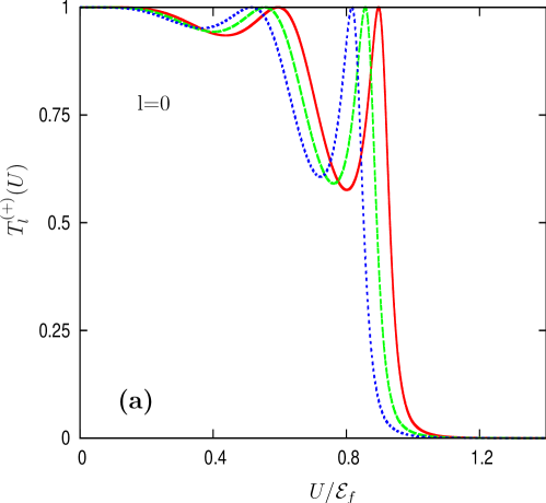
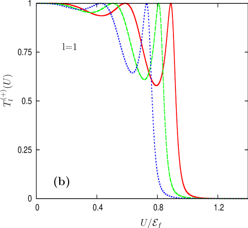
Figure 3: ( (Color online) Transmission probabilities for incident electrons in the the “$+$” state as functions of the potential height $U$ for three values of SOI energy ${\cal E}_{\alpha}$ for (a) $l=0$ and (b) $l=1$. Here, ${\cal E}_{\alpha}=0$ (solid line), $0.04{\cal E}_{f}$ (dashed line) and $0.08{\cal E}_{f}$ (dotted line) where the incident energy $E^{i}={\cal E}_{f}$.

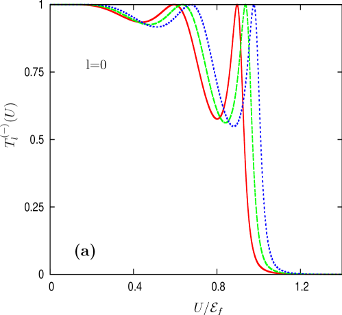
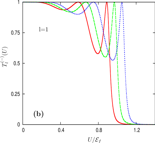
Figure 4: (Color online) Transmission probabilities for electrons in the “$-$” state as functions of the height $U$ of the potential barrier for three values of SOI energy ${\cal E}_{\alpha}$, In (a) $l=0$ and (b) $l=1$ and we chose ${\cal E}_{\alpha}=0$ (solid line), $0.04{\cal E}_{f}$ (dashed line) and $0.08{\cal E}_{f}$ (dotted line).

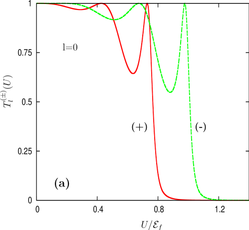
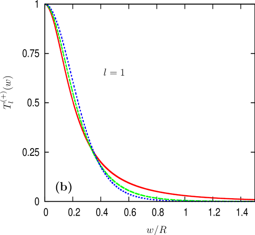
Figure 5: (Color online) (a) Comparison of the transmission probabilities between “$+$” and “$-$” states for ${\cal E}_{\alpha}=0.08{\cal E}_{f}$ and angular momentum quantum number $l=0$. (b) The dependence of the transmission probability on the width of the barrier $w$ in units of $R$ the radius of the nanotube ($R=10$nm) for “$+$” state. We chose ${\cal E}_{\alpha}=0$ (solid line), $0.04{\cal E}_{f}$ (dashed line) and $0.08{\cal E}_{f}$ (dotted line).

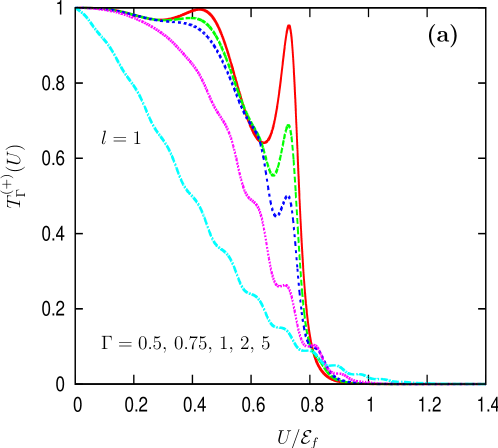
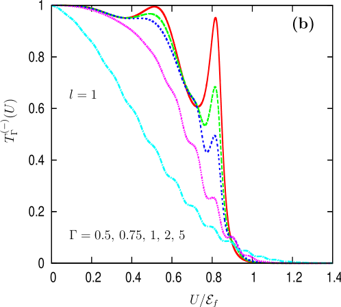
Figure 6: (Color online) Transmission probabilities in the presence of impurities (defects) included phenomenologically via Eq. (66) with the parameter $\Gamma$ related to temperature for (a) the $``+$” states and (b) the $``-"$ for SOI ${\cal E}_{\alpha}=0.08{\cal E}_{f}$.

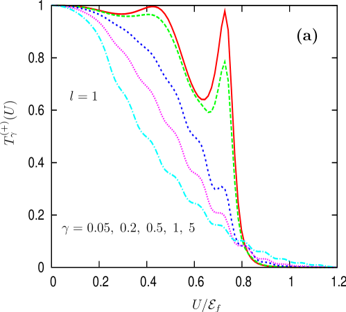
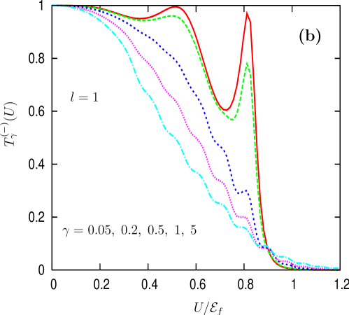
Figure 7: (Color online) Transmission Probabilities in the presence of impurities (defects) included phenomenologically via Eq. (67) with the parameter $\gamma$ related to temperature for (a) the $``+$” states and (b) the $``-"$ for SOI ${\cal E}_{\alpha}=0.08{\cal E}_{f}$.

- (1) J. Nitta, T. Akazaki, H. Takayanagi, and T. Enoki, Phys. Rev. Lett. 78, 1335 (1997).
- (2) Godfrey Gumbs, Phys. Rev. B73, 165315 (2006).
- (3) A. De Martino and R. Egger, J. Phys.: Condensed Matter 17, 5523-5532 (2005).
- (4) Daniel Huertas-Hernando, F. Guinea, and Arne Brataas, Phys. Rev. B74, 155426 (2006).
- (5) C. L. Kane and E. J. Mele, Phys. Rev. Lett. 95, 226801 (2005).
- (6) Hongki Min, J. E. Hill, N. A. Sinitsyn, B. R. Sahu, Leonard Kleinman, and A. H. MacDonald, Phys. Rev. B 74, 165310 (2006).
- (7) M. Mason, M. J. Biercuk, and C. M. Marcus, Science 303, 655 (2004).
- (8) K. Tsukagoshi,B. W. Alphenaar, and H. Ago, Nature 401, 572 (1999).
- (9) B. Zhao, I. Mnch, H. Vinzelberg, T. Mhl, and C. M. Schneider, Appl. Phys. Lett. 80, 3144 (2002).
- (10) Godfrey Gumbs, Yonatan Abranyos and Tibab McNeish, Journal of Phys. Condens. Matter 19, 106213 (2007).
- (11) Godfrey Gumbs and Yonatan Abranyos, Phys. Rev. A70, 050302 (2004).
- (12) J. Shi, P. Zhang, D. Xiao, and Q. Niu, Phys. Rev. Lett. 96, 076604 (2006).
- (13) N. Mason, M. J. Biercuk, C. M. Marcus, Science 303, 655 (2004).
- (14) Prashant Sharma, Science 307, 531 (2005).
- (15) V. A. Sablikov and Y. Ya. Tkach, Phys. Rev. B76, 245321 (2007).
- (16) Yurii Ya Tkach, Vladimir A Sablikov, and Aleksei A Sukhanov, J. Phys.: Condens. Matter 21, 125801 (2009).
- (17) Aleksei A Sukhanov, Vladimir A Sablikov and Yurii Ya Tkach, Journal of Phys. Condensed Matter 21, 375801 (2009).
- (18) Vladimir A. Sablikov, Aleksei A. Sukhanov, and Yurii Ya. Tkach, Phys. Rev. B78, 153302 (2008).
- (19) I.K. Marmorkos and S. Das Sarma, Phys. Rev. B 45, 13396 (1992).
- (20) D. W. Wang and S. Das Sarma, Phys. Rev. B65, 035103 (2001).
- (21) Chu-Wei Jiang, Martin A. Green, Eun-Chel Cho, and Gavin Conibeer, Jour. Appl. Phys. 96, 5006 (2004).
- (22) L. El Mir and J. C. Bourgoin, Phys. Stat. Sol. (b) 207, 577 (1998).
- (23) B. Scharf, J. Fabian, and A. Matos-Abiague, Phys. Rev. B81, 125428 (2010).
- (24) Godfrey Gumbs and Antonios Balassis, Phys. Rev. B71, 235410 (2005).