Scattering universality classes of side jump in anomalous Hall effect

Abstract

The anomalous Hall conductivity has an important extrinsic contribution known as side jump contribution, which is independent of both scattering strength and disorder density. Nevertheless, we discover that side jump has strong dependence on the spin structure of the scattering potential. We propose three universality classes of scattering for the side jump contribution, having the characters of being spin-independent, spin-conserving and spin-flip respectively. For each individual class, the side jump contribution takes a different unique value. When two or more classes of scattering are present, the value of side jump is no longer fixed but varies as a function of their relative disorder strength. As system control parameter such as temperature changes, due to the competition between different classes of disorder scattering, the side jump Hall conductivity could flow from one class dominated limit to another class dominated limit. Our result indicates that magnon scattering plays a role distinct from normal impurity scattering and phonon scattering in the anomalous Hall effect because they belong to different scattering classes.

I INTRODUCTION

The anomalous Hall effect (AHE), in which a transverse voltage is induced by a longitudinal current flow in ferromagnetic materials, is one of the most intriguing effects in condensed matter physics. While it has been widely used experimentally as a standard technique for the characterization of ferromagnet materials, the theoretical formulation of AHE proves to be complicated and is a subject full of controversial issues and conflicting results. naga2009 In recent years, an important connection has been established between AHE and the Berry phase of Bloch electrons. berr1984 ; sund1999 ; jung2002 ; onod2002 This triggers revived interest in this subject and is followed by extensive researches both theoretically and experimentally.ye1999 ; tagu2001 ; crep2001 ; fang2003 ; culc2003 ; schl2003 ; sino2004 ; yao2004 ; hald2004 ; lee2004 ; sini2005 ; duga2005 ; kotz2005 ; zeng2006 ; liu2006 ; inou2006 ; onod2006 ; yao2007 ; sini2007prb ; boru2007 ; kato2007 ; nunn2007 ; liu2007 ; sini2008 ; onod2008 ; nunn2008 ; rash2008 ; venk2008 ; arse2008 ; kova2009 ; sang2009 ; shio2009 ; glun2009 ; tian2009 ; sino2010 ; dimi2010

It is now generally accepted that spin-orbit coupling and spin splitting are two essential ingredients for AHE, and apart from an intrinsic contribution which is scattering independent, there are also important extrinsic contributions to AHE due to disorder scattering. Based on their parametric dependence on the disorder density $n_{\text{dis}}$, the extrinsic contributions can be collected into two subgroups: the side jump contribution of order $n_{\text{dis}}^{0}$ and the skew scattering contribution of order $n_{\text{dis}}^{-1}$.

The side jump contribution is of special interest in that it arises from scattering, but surprisingly it does not depend on either the scattering strength or the disorder density (we shall use the term “disorder strength” to stand for both scattering strength and disorder density). Theoretical calculations of simple model systems show that the side jump contribution is usually at least as important as intrinsic contribution.sini2005 ; duga2005 ; onod2006 ; sini2007prb However, the good agreement between the intrinsic contribution calculated from first principles and the experimental results seems to indicate that the side jump contribution only plays a subdominant role.yao2004 ; zeng2006 This remains as a puzzle that need to be resolved and is partly our motivation for the present work.

Historically, the concept of side jump was first devised by Berger,berg1970 which refers to the coordinate shift of a wave-packet during an impurity scattering and this process leads to a contribution of order $n_{\text{dis}}^{0}$ to the anomalous Hall conductivity. Recently, it has been found that besides this coordinate shift process, several other scattering processes also generate contributions of order $n_{\text{dis}}^{0}$.sini2007prb It should be noted that the term “side jump” used in the present paper includes all the scattering induced contributions of order $n_{\text{dis}}^{0}$, not only the contribution from Berger’s original side jump.

In the study of physical systems, properties which are insensitive to detailed parameter values and system configurations but are only determined by the symmetry are especially interesting and important. It is helpful to define universality classes based on the behavior of these universal properties under certain imposed symmetry and study the generic properties of each class. Side jump can be regarded as a universal property for a disordered system in the sense that its value does not depend on the detailed disorder profile, but we shall see that it has sensitive dependence on the symmetry property of the scattering. Consequently, it is natural to define universality classes of disorder scattering according to their side jump contributions and study the anomalous Hall response for each class.

In this work, we propose three universality classes of disorder scattering, each has different structures in spin space. We find that: (1) for each individual class, the side jump contribution takes a distinct value independent of the detailed disorder profile. In particular, we show that magnon scattering plays a distinct role from both impurity scattering and phonon scattering in AHE; (2) when several classes of scattering are present, side jump depends on their relative disorder strength and a sign change is possible as a result of their competition. Since in real physical system scattering processes of all the three classes exist, our finding indicates that a careful classification and analysis of different scattering processes is indispensible for an accurate account of AHE.

This paper is organized as the following. First, in Sec. II, we propose and discuss the three scattering universality classes of side jump. In Sec. III we demonstrate our ideas by a concrete analytical calculation of anomalous Hall conductivity of massive Dirac model for each universality class. In Sec. IV we discuss the important consequences of our result, especially about contribution from magnon scattering in AHE, and draw some final conclusions.

II UNIVERSALITY CLASSES OF DISORDER SCATTERING

The general form of a random disorder potential for carriers with spin (or pseudospin) degrees of freedom can be written as

$$\hat{V}_{\text{dis}}(\bm{r})=\sum_{i}\left[V_{0}(\bm{r}-\bm{R}_{i})+\bm{V}(\bm{r}-\bm{R}_{i})\cdot\hat{\bm{\sigma}}\right],$$ (1)

where $\bm{R}_{i}$ ($i=1,2,\cdots$) are the positions of randomly distributed scattering centers, $\hat{\bm{\sigma}}=(\hat{\sigma}_{x},\hat{\sigma}_{y},\hat{\sigma}_{z})$ is a vector with components of Pauli matrices and the hat means the quantity is a $2\times 2$ matrix in spin space. We assume that the statistical average of the disorder potential is zero (any nonzero value only shifts the origin of total energy) and the second order spatial correlation only depends on the difference in positions,

$$\langle V_{\text{dis}}(\bm{r})\rangle_{c}=0,\qquad\langle V_{\text{dis}}(\bm{r})V_{\text{dis}}(\bm{r}^{\prime})\rangle_{c}=B(\bm{r}-\bm{r}^{\prime}),$$ (2)

where the angular bracket $\langle\cdots\rangle_{c}$ denotes disorder average. In order to discuss skew scattering which originates from higher order scattering processes, we allow a non-vanishing third order disorder correlation instead of requiring the disorder to be purely Gaussian.

Time reversal symmetry has to be broken for the appearance of AHE.naga2009 In ferromagnet, this is realized by the spontaneous magnetic ordering. We will be most interested in the configuration that the magnetization is perpendicular to the two-dimensional (2D) plane where the transport occurs, as is pertinent for most experimental investigations. It is reasonable to assume that over disorder average the system is isotropic in the 2D plane with no preferred in-plane directions. With this symmetry constraint, the total angular momentum (in the direction normal to the plane which we will refer to as $z$-axis) of the carriers are conserved on average. Due to spin-orbit coupling, the carrier’s orbital motion which is tied to orbital angular momentum depends sensitively on the change of its spin angular momentum during a scattering. Based on this consideration, we propose the following three classes of disorder scattering which as we will see lead to different values of side jump contribution:

$$\begin{split}&\text{Class A}\qquad\hat{V}=V^{\text{o}}\hat{1},\\ &\text{Class B}\qquad\hat{V}=V^{\text{o}}\hat{\sigma}_{z},\\ &\text{Class C}\qquad\hat{V}=V^{\text{o}}\hat{\sigma}_{\pm}/\sqrt{2},\\ \end{split}$$ (3)

where $V^{\text{o}}$ denotes the orbital part of the scattering potential, and $\hat{\sigma}_{\pm}\equiv\hat{\sigma}_{x}\pm i\hat{\sigma}_{y}$. Each class has a different action on the carrier’s spin. Class A is isotropic in spin space. Class B, like Class A, conserve the $z$-component of the carrier spin but spin up and spin down carriers experience different scattering potentials. Class C, unlike the first two classes, induces spin flips. The three classes as we discuss later represent a quite general classification scheme for real physical systems. This classification scheme is also evident if we consider the disorder correlation function under the in-plane rotational symmetry,expl

$$\begin{split}\left\langle V_{\text{dis}}^{ij}(\bm{r})V_{\text{dis}}^{ji}(\bm{r}^{\prime})\right\rangle_{c}=\;&\langle V_{0}V_{0}\rangle_{c}\delta_{ij}+\langle V_{z}V_{z}\rangle_{c}(\hat{\sigma}_{z})_{ij}(\hat{\sigma}_{z})_{ji}\\ &+\sum_{\alpha=x,y}\langle V_{\alpha}V_{\alpha}\rangle_{c}(\hat{\sigma}_{\alpha})_{ij}(\hat{\sigma}_{\alpha})_{ji},\end{split}$$ (4)

where $i,j$ are spin indices. Since $\langle V_{x}V_{x}\rangle_{c}=\langle V_{y}V_{y}\rangle_{c}$ due to the in-plane rotational symmetry, the last term is proportional to

$$\left[(\hat{\sigma}_{+})_{ij}(\hat{\sigma}_{-})_{ji}+(\hat{\sigma}_{-})_{ij}(\hat{\sigma}_{+})_{ji}\right],$$ (5)

with each term being invariant under spin rotations around $z$-axis. The three terms in Eq.(4) just correspond to the three classes we defined.

Before proceeding, we point out an important difference between Class C and Class A, B on their third order correlation functions. The Class C disorder can be expressed as $\bm{V}(\bm{r})\cdot\bm{\sigma}$ where $\bm{V}$ is a random in-plane vector. Under in-plane rotational symmetry, $\bm{V}$ has no preferred direction therefore its third order correlation like $\langle VVV\rangle_{c}$ must vanish. However for Class A or Class B, the third order correlation is not dictated by this symmetry constraint hence does not necessarily vanish. This difference will be reflected in the skew scattering contribution to the AHE.

The transverse motion of carriers in AHE is a result of spin-orbit coupling. In our classification scheme, each class of scattering has different effects on the carrier spin, hence will also have different effects on the carrier orbits. This is the underlying reason for their distinct contributions to the AHE and especially the side jump part. In the following section, we demonstrate this idea by a concrete model calculation.

III AHE OF MASSIVE DIRAC MODEL

III.1 Model and Approach

To demonstrate the rationale of our classification scheme, we calculate the anomalous Hall conductivity for the massive Dirac model. This model is usually considered as the minimal model for AHE.naga2009 The model Hamiltonian reads (we set $\hbar=1$ and assume $\Delta>0$ in the following calculations)

$$\hat{\mathcal{H}}=v(k_{x}\hat{\sigma}_{x}+k_{y}\hat{\sigma}_{y})+\Delta\hat{\sigma}_{z},$$ (6)

where spin-orbit coupling is contained in the first term with $v$ being the coupling constant, and the last term breaks the time reversal symmetry and is also responsible for the finite electron mass at the band edge. This model captures interesting physics near a generic band anti-crossing point due to spin-orbit coupling.

The eigenstates of the system are

$$\psi_{\bm{k}}^{\pm}(\bm{r})=\frac{1}{\sqrt{A}}e^{i\bm{k}\cdot\bm{r}}|u_{\bm{k}}^{\pm}\rangle,$$ (7)

with the corresponding energy eigenvalues

$$\varepsilon^{\pm}(\bm{k})=\pm\sqrt{(vk)^{2}+\Delta^{2}},$$ (8)

where $\pm$ labels the upper and lower band respectively, $A$ is the system size, and $|u_{\bm{k}}^{\pm}\rangle$ is the spin part of the eigenstate which can be written as

$$|u_{\bm{k}}^{+}\rangle=\left(\begin{array}[]{c}\cos\frac{\theta}{2}\\ \sin\frac{\theta}{2}e^{i\phi}\\ \end{array}\right),\qquad|u^{-}_{\bm{k}}\rangle=\left(\begin{array}[]{c}\sin\frac{\theta}{2}\\ -\cos\frac{\theta}{2}e^{i\phi}\\ \end{array}\right),$$ (9)

where $\theta$ and $\phi$ are the spherical angles of the vector $(vk_{x},vk_{y},\Delta)$ such that

$$\begin{split}&\cos\theta=\frac{\Delta}{\sqrt{(vk)^{2}+\Delta^{2}}},\qquad\sin\theta=\frac{vk}{\sqrt{(vk)^{2}+\Delta^{2}}},\\ &\tan\phi=k_{y}/k_{x}.\end{split}$$ (10)

Due to spin-orbit coupling, the spin state is a function of the momentum $\bm{k}$. The energy spectrum consists of two anti-crossing bands with a band gap of $2\Delta$. From the dispersion relation Eq.(8), the geometry of the bands can be termed as a “Dirac hyperboloid” (of two sheets).

To calculate the anomalous Hall conductivity, we follow Sinitsyn et al.sini2007prb by using the Kubo-Streda formalism.stre1982 ; crep2001 In this approach, the Hall conductivity can be separated into two parts in the weak scattering regime, $\sigma_{xy}=\sigma_{xy}^{\text{I}}+\sigma_{xy}^{\text{II}}$, where $\sigma_{xy}^{\text{I}}$ is a Fermi surface contribution which includes all the important scattering contributions, and $\sigma_{xy}^{\text{II}}$ is a Fermi sea contribution for which we only need to retain the scattering-free component. sini2007prb In the following we consider that the system is electron doped with Fermi energy $\varepsilon_{F}>\Delta$ and due to particle-hole symmetry, the results can be easily generalized to the hole-doped case. We assume that the system is in the weak scattering regime, i.e. $k_{F}l\gg 1$ where $k_{F}$ is the Fermi wave vector and $l$ is the electron mean free path. It has been found that $\sigma_{xy}^{\text{II}}$ vanishes sini2007prb and the task gets reduced to the evaluation of $\sigma_{xy}^{\text{I}}$ which is given by the following expression

$$\sigma_{xy}^{\text{I}}=\frac{e^{2}}{2\pi A}\text{Tr}\left\langle\hat{v}_{x}\hat{G}^{R}(\varepsilon_{F})\hat{v}_{y}\hat{G}^{A}(\varepsilon_{F})\right\rangle_{c},$$ (11)

where $\hat{G}^{R}$ and $\hat{G}^{A}$ are the retarded and advanced Green’s functions respectively, $\hat{v}_{x}$ and $\hat{v}_{y}$ are the velocity operators, and the trace is taken over both momentum and spin spaces. In weak scattering regime, the calculation is performed perturbatively in the small parameter $1/(k_{F}l)$.

In our model, we consider the scattering processes to be quasi-elastic, hence the disorder lines in Feynman diagrams carry no energy arguments. This serves as a good approximation for the scattering by collective excitations such as phonons or magnons as long as energy of collective excitation involved in the scattering is much less than the Fermi energy. Since the typical energy scale of excitations is $k_{B}T$, this condition is satisfied for temperatures with $k_{B}T\ll\varepsilon_{F}$. Furthermore, for massless excitation with a spectrum $\omega(k)=v_{q}k$ ($v_{q}$ is a constant sound speed), quasi-elastic approximation is justified even at higher temperatures if the quasi-particle speed $v_{q}$ is much less than $v_{F}$, viz the band velocity at Fermi level. For massive quasi-particle excitations, its validity can be justified if the quasi-particle mass is much larger than the electron effective mass.

In the following, we calculate the Hall conductivity for each individual class, or equivalently when one class of scattering is dominant. The evaluation of the conductivity follows standard procedures, and the relevant Feynman diagrams under self-consistent non-cross approximation have been identified before, sini2007prb so we do not elaborate here. The results are listed below.

III.2 Intrinsic Contribution

The intrinsic contribution of AHE is a property purely of the spin-orbit coupled band structure. It was first proposed by Karplus and Luttinger,karp1954 and recently its connection with the Berry phase of Bloch electrons is established.jung2002 ; onod2002 It is now understood that spin-orbit coupled bands usually possess effective magnetic fields in momentum space known as Berry curvatures,sund1999 which deflect carriers in the transverse directions. The intrinsic contribution of anomalous Hall conductivity equals the integration of Berry curvatures of all the occupied states. Because it does not depend on scattering, intrinsic contribution is the same for all the three universality classes. In Kubo-Streda formalism, intrinsic contribution is the sum of the scattering-free part of $\sigma_{xy}^{\text{I}}$ and $\sigma_{xy}^{\text{II}}$.

For electron doped case, we can separate the intrinsic Hall conductivity $\sigma^{\text{int}}_{xy}$ into two parts,

$$\sigma^{\text{int}}_{xy}=\sigma^{\text{int(v)}}_{xy}+\sigma^{\text{int(c)}}_{xy},$$ (12)

where $\sigma^{\text{int(v)}}_{xy}$ is the contribution from all the completely occupied valence bands below the Fermi surface and $\sigma^{\text{int(c)}}_{xy}$ is the contribution from the partially filled conduction band where the Fermi surface lies in. The contribution from completely filled bands $\sigma^{\text{int(v)}}_{xy}$ must be a topologically quantized value $Ce^{2}/(2\pi)$ with $C$ being an integer called the first Chern number.naga2009 The lower band of the massive Dirac model has a contribution of $-e^{2}/4\pi$. This is not a contradiction because the Dirac band is not bounded. For any real physical system, the evaluation of $C$ must go beyond the low energy effective model and require complete information of the entire Fermi sea. On the contrary, the contribution $\sigma^{\text{int(c)}}_{xy}$ from the partially filled conduction band can be regarded as a Fermi surface propertyhald2004 and is captured within the effective model,

$$\sigma^{\text{int(c)}}_{xy}=\frac{e^{2}}{4\pi}(1-\cos\theta_{F}),$$ (13)

where $\theta_{F}$ is the spherical angle $\theta$ at the Fermi surface when $k=k_{F}$.

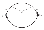
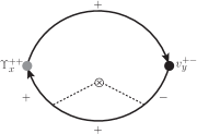
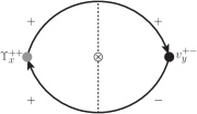
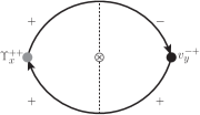
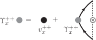
Figure 1: (a)-(d) are the four conductivity diagrams of side jump that correspond to the distribution function correction. $+$ and $-$ represent the upper and lower band respectively. $\Upsilon$ stands for the renormalized velocity vertex which is dressed by a ladder like diagram as shown in (e).

III.3 Side Jump Contribution

Now let’s focus on the side jump contribution which is the central quantity we are interested in. For each individual class, it is independent of disorder density $n_{\text{dis}}$ and scattering strength $V^{\text{o}}$. It can be expressed in terms of $\theta_{F}$ and a set of scattering times defined on the Fermi surface. For notational convenience, we define

$$\frac{1}{\tau_{i}}\equiv 2\pi n_{\text{dis}}\int\frac{d^{2}\bm{k}^{\prime}}{(2\pi)^{2}}\left|V_{\bm{k^{\prime}k}}^{\text{o}}\right|^{2}\cos^{i}(\phi-\phi^{\prime})\delta(\varepsilon_{F}-\varepsilon_{\bm{k}^{\prime}}^{+}),$$ (14)

where $V_{\bm{k^{\prime}k}}^{\text{o}}=\langle\bm{k}^{\prime}|V^{\text{o}}|\bm{k}\rangle$ is the matrix element of the orbital part of the scattering potential in momentum space and $i=0,1,2,\cdots$ is an integer.

In the semiclassical picture, the side jump we defined here consists of three components: a contribution from the coordinate shift (the original Berger’s side jump), a contribution from a correction of distribution function (called the anomalous distribution), and a contribution from some higher order scattering processes (called the intrinsic skew scattering). The first two components are shown to be equal. sini2007prb In the Kubo-Streda approach, Fig. 1 shows a set of diagrams that contributes to the side jump in the chiral (eigenstate) basis. These correspond to the contribution from the anomalous distribution function correction, i.e. the second component above. The diagrams corresponding to the contribution from coordinate shift can be obtained by simply exchanging the subscripts $x$ and $y$ in Fig. 1 and further making a $180^{\circ}$ rotation (i.e. exchanging $G^{R}$ and $G^{A}$). The resulting contribution to Hall conductivity from these two components for each scattering class is

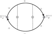
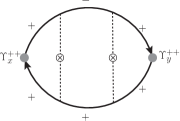
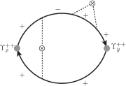
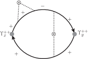
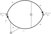
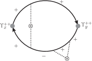
Figure 2: The diagrams corresponding to the part of side jump from fourth order scattering process (intrinsic skew scattering).

$$\begin{split}&\text{Class A}:\qquad\sigma^{\text{sj(a)}}_{xy}=-\frac{e^{2}}{2\pi}\frac{\sin^{2}\theta_{F}\cos\theta_{F}(\tau_{0}^{-1}-\tau_{1}^{-1})}{(1+\cos^{2}\theta_{F})\tau_{0}^{-1}-2\cos^{2}\theta_{F}\tau_{1}^{-1}-\sin^{2}\theta_{F}\tau_{2}^{-1}},\\ &\text{Class B}:\qquad\sigma^{\text{sj(a)}}_{xy}=0,\\ &\text{Class C}:\qquad\sigma^{\text{sj(a)}}_{xy}=\frac{e^{2}}{4\pi}\cos\theta_{F}.\end{split}$$ (15)

We observe that different scattering class contributes very differently to the Hall conductivity. In the diagramatic approach, this difference originates from the different $\bm{k}$ dependence at scattering vertices, which in turn results from their different spin structures. It should be noted that the vanishing value of class B is not a general feature but rather depends on the specific model we considered here.classB

The third component (intrinsic skew scattering) results from certain fourth order scattering processes. The corresponding diagrams are shown in Fig. 2 and the results are

$$\begin{split}&\text{Class A}:\qquad\sigma^{\text{sj(b)}}_{xy}=-\frac{e^{2}}{4\pi}\frac{\sin^{4}\theta_{F}\cos\theta_{F}(\tau_{0}^{-1}-\tau_{2}^{-1})(\tau_{0}^{-1}-2\tau_{1}^{-1}+\tau_{2}^{-1})}{\left[(1+\cos^{2}\theta_{F})\tau_{0}^{-1}-2\cos^{2}\theta_{F}\tau_{1}^{-1}-\sin^{2}\theta_{F}\tau_{2}^{-1}\right]^{2}},\\ &\text{Class B}:\qquad\sigma^{\text{sj(b)}}_{xy}=\frac{e^{2}}{4\pi}\frac{\sin^{4}\theta_{F}\cos\theta_{F}(\tau_{0}^{-1}-\tau_{2}^{-1})^{2}}{\left[(1+\cos^{2}\theta_{F})\tau_{0}^{-1}-2\tau_{1}^{-1}+\sin^{2}\theta_{F}\tau_{2}^{-1}\right]^{2}},\\ &\text{Class C}:\qquad\sigma^{\text{sj(b)}}_{xy}=0.\end{split}$$ (16)

The $\sigma^{\text{sj(b)}}_{xy}$ contribution vanishes for class C is a very general result because each such diagram contains a factor of the form $\int\sin\phi\text{d}\phi$ from the momentum integral at the velocity vertex which suppresses the intrinsic skew scattering process.

The total side jump contribution to anomalous Hall conductivity is given by $\sigma^{\text{sj}}_{xy}=\sigma^{\text{sj(a)}}_{xy}+\sigma^{\text{sj(b)}}_{xy}$. It is clear that each class has a distinct side jump contribution. Scattering rates with the same power appear in both nominator and denominator of the expressions in Eqs.(LABEL:sj,LABEL:isk), hence the results are independent of disorder density and scattering strength. The dependence on the band parameters such as $\Delta$ and $\varepsilon_{F}$ are also different for different classes. Furthermore, it should be noted that different classes can have side jump contribution with different signs, as shown here between Class A and the other two classes.

III.4 Skew Scattering Contribution

Although our focus is the side jump contribution, to be complete, we also calculated the skew scattering contribution for each scattering class. In the semiclassical picture, skew scattering contribution comes from the asymmetric part of the scattering rates for higher order scattering processes. The leading contribution is related to the third order disorder correlation and has a $n_{\text{dis}}^{-1}$ dependence.fourth The corresponding Feynman diagrams are shown in Fig. 3 and the skew scattering contribution to Hall conductivity for each class is given by

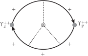
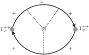
Figure 3: The two diagrams corresponding to skew scattering contribution.

$$\begin{split}&\text{Class A}:\qquad\sigma^{\text{sk}}_{xy}=-\frac{e^{2}}{2\pi}\frac{\sin^{4}\theta_{F}\cos\theta_{F}\tau_{\text{sk}}^{-2}}{\left[(1+\cos^{2}\theta_{F})\tau_{0}^{-1}-2\cos^{2}\theta_{F}\tau_{1}^{-1}-\sin^{2}\theta_{F}\tau_{2}^{-1}\right]^{2}},\\ &\text{Class B}:\qquad\sigma^{\text{sk}}_{xy}=\frac{e^{2}}{2\pi}\frac{\sin^{4}\theta_{F}\tau_{\text{sk}}^{-2}}{\left[(1+\cos^{2}\theta_{F})\tau_{0}^{-1}-2\tau_{1}^{-1}+\sin^{2}\theta_{F}\tau_{2}^{-1}\right]^{2}},\\ &\text{Class C}:\qquad\sigma^{\text{sk}}_{xy}=0.\end{split}$$ (17)

where

$$\begin{split}\frac{1}{\tau_{\text{sk}}^{2}}\equiv 2\pi\varepsilon_{F}n_{\text{dis}}\int\frac{d^{2}\bm{k}^{\prime}}{(2\pi)^{2}}&\int\frac{d^{2}\bm{k}^{\prime\prime}}{(2\pi)^{2}}\langle V_{\bm{kk^{\prime}}}^{\text{o}}V_{\bm{k^{\prime}k^{\prime\prime}}}^{\text{o}}V_{\bm{k^{\prime\prime}k}}^{\text{o}}\rangle_{c}\sin(\phi^{\prime}-\phi)\\ &\cdot\left[\sin(\phi-\phi^{\prime\prime})+\sin(\phi^{\prime\prime}-\phi^{\prime})+\sin(\phi^{\prime}-\phi)\frac{}{}\right]\cdot\delta(\varepsilon_{F}-\varepsilon^{+}_{\bm{k}^{\prime}})\delta(\varepsilon_{F}-\varepsilon^{+}_{\bm{k}^{\prime\prime}}).\end{split}$$ (18)

Note that the factor $1/\tau_{\text{sk}}^{2}$ is proportional to $n_{\text{dis}}$, hence $\sigma^{\text{sk}}_{xy}$ is of order $n_{\text{dis}}^{-1}$. Because the third order disorder correlation vanishes for Class C as we discussed in Sec.II, $1/\tau_{\text{sk,C}}^{2}=0$ and the skew scattering process is forbidden for this type of disorder scattering. Therefore, we see an important qualitative difference of the anomalous Hall response for Class C and the other two classes: in the weak scattering regime, the leading contribution for Class A and Class B is the skew scattering of order $n^{-1}_{\text{dis}}$, but for Class C the leading contribution is the intrinsic plus side jump which are of order $n^{0}_{\text{dis}}$.

III.5 Total Hall Conductivity of Order $n_{\text{dis}}^{0}$

The above results are valid for disorder scattering with general orbital part. If we consider the simple white noise (short range) disorders, the results for Hall conductivity are greatly simplified. In this case, we have for each class

$$\frac{1}{\tau_{1}}=0,\qquad\frac{1}{\tau_{2}}=\frac{1}{2\tau_{0}}.$$ (19)

Then the total Hall conductivity can be written as ($\sigma_{xy}^{\text{int(v)}}$ is not included here, as discussed in Sec.III.B):
Class A:

$$\begin{split}\sigma_{xy}=&\frac{e^{2}}{4\pi}(1-\cos\theta_{F})-\frac{e^{2}}{\pi}\frac{\sin^{2}\theta_{F}\cos\theta_{F}}{1+3\cos^{2}\theta_{F}}\\ &-\frac{3e^{2}}{4\pi}\frac{\sin^{4}\theta_{F}\cos\theta_{F}}{(1+3\cos^{2}\theta_{F})^{2}}-\frac{2e^{2}}{\pi}\frac{\sin^{4}\theta_{F}\cos\theta_{F}}{(1+3\cos^{2}\theta_{F})^{2}}\frac{\tau_{\text{sk}}^{-2}}{\tau_{0}^{-2}}.\end{split}$$ (20)

Class B:

$$\begin{split}\sigma_{xy}=&\frac{e^{2}}{4\pi}(1-\cos\theta_{F})+\frac{e^{2}}{4\pi}\frac{\sin^{4}\theta_{F}\cos\theta_{F}}{(3+\cos^{2}\theta_{F})^{2}}\\ &+\frac{2e^{2}}{\pi}\frac{\sin^{4}\theta_{F}}{(3+\cos^{2}\theta_{F})^{2}}\frac{\tau_{\text{sk}}^{-2}}{\tau_{0}^{-2}}.\end{split}$$ (21)

Class C:

$$\begin{split}\sigma_{xy}=&\frac{e^{2}}{4\pi}.\end{split}$$ (22)

The expression in Eq.(20) recovers the result obtain by Sinitsyn et al.sini2007prb Clearly, each universality class has its distinct extrinsic Hall conductivity and different functional dependence on the system parameters such as $\theta_{F}$. Note that for class C, the side jump contribution cancels with the part of intrinsic contribution which depends on the Fermi energy, making the final result a constant and the value is the same as the intrinsic contribution for a completely filled conduction band (i.e. in the limit $\theta_{F}\rightarrow\pi/2$). We have checked that this interesting cancelation occurs for a generic class of Hamiltonians $\mathcal{H}=vk^{n}[\cos(n\phi_{\bm{k}})\sigma_{x}+\sin(n\phi_{\bm{k}})\sigma_{y}]+\Delta\sigma_{z}$ where $n$ is an integer.

Here we are most interested in the part of Hall conductivity $\sigma_{xy}^{0}$ that is of order $n_{\text{dis}}^{0}$. This includes the intrinsic contribution and the side jump contribution, i.e.

$$\sigma^{0}_{xy}=\sigma^{\text{int}}_{xy}+\sigma^{\text{sj}}_{xy}.$$ (23)

In Fig. 4, for each scattering class (with white noise spatial correlation), we plot $\sigma^{0}_{xy}$ as a function of Fermi energy $\varepsilon_{F}$ for the massive Dirac model. Observe that $\sigma^{0}_{xy}$ for class C takes a constant value $e^{2}/4\pi$ which is independent of Fermi energy and the curves for both class A and class B approach this constant value asymptotically as $\varepsilon_{F}\rightarrow\infty$. For class A, the extrinsic contribution has opposite sign as compared with the the intrinsic contribution. Because of this sign difference, the Hall conductivity for class A takes negative values for Fermi energies below $\varepsilon_{F}\approx 7.3\Delta$. This behavior differs from that for class B and class C whose extrinsic contributions have the same sign as the intrinsic contribution, so their overall $\sigma_{xy}^{0}$’s are positive. This shows that the Hall conductivity sensitively depends on the class of disorder scattering.

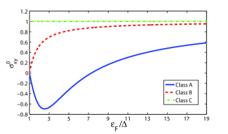
Figure 4: (color online). $\sigma^{0}_{xy}$ plotted as a function of the Fermi energy $\varepsilon_{F}$ for each of the three universality classes. $\sigma^{0}_{xy}$ is measured in units of $e^{2}/(4\pi)$, and $\varepsilon_{F}$ is measured in units of $\Delta$ which is half of the band gap.

III.6 Competition between Classes

In the presence of two or more classes of scattering, there will be a competition between them in the anomalous Hall response. The resulting side jump contribution takes the following generic form:

$$\sigma^{\text{sj}}_{xy}=\frac{\sum_{\alpha}a_{\alpha}\tau_{\alpha}^{-1}}{\sum_{\alpha}b_{\alpha}\tau_{\alpha}^{-1}}+\frac{\sum_{\alpha\beta}c_{\alpha\beta}\tau_{\alpha}^{-1}\tau_{\beta}^{-1}}{\sum_{\alpha\beta}d_{\alpha\beta}\tau_{\alpha}^{-1}\tau_{\beta}^{-1}},$$ (24)

where the $\tau_{\alpha(\beta)}$ is the scattering time defined for each class of scattering involved, $a_{\alpha}$, $b_{\alpha}$, $c_{\alpha\beta}$ and $d_{\alpha\beta}$ are the (disorder independent) coefficients which depend only on system intrinsic parameters such as $\theta_{F}$ in the present model.

As an example, let’s consider the competition between Class A and Class C. The calculation is tedious but straightforward. The resulting total Hall conductivity can be expressed as

$$\sigma_{xy}=\frac{e^{2}}{4\pi}(1-\cos\theta_{F})-\frac{e^{2}}{\pi}\frac{\sin^{2}\theta_{F}\cos\theta_{F}(1-\zeta)}{(1+3\cos^{2}\theta_{F})+4\sin^{2}\theta_{F}\zeta}-\frac{e^{2}}{\pi}\frac{\sin^{4}\theta_{F}\cos\theta_{F}(\frac{3}{4}-\zeta+2\eta)}{\left[(1+3\cos^{2}\theta_{F})+4\sin^{2}\theta_{F}\zeta\right]^{2}},$$ (25)

where the parameter $\zeta$ defined as $\zeta\equiv(\tau_{0C}^{-1}-\tau_{1C}^{-1})/(\tau_{0A}^{-1}-\tau_{1A}^{-1})$ is a measure of the relative disorder strength of the two classes, and $\eta\equiv\tau_{\text{sk},A}^{-2}/(\tau_{0A}^{-1}-\tau_{1A}^{-1})^{2}$ is a factor for skew scattering contribution from Class A, here $\tau_{iA}$ stands for the scattering time $\tau_{i}$ defined in Eq.(14) for Class A scattering and $\tau_{iC}$ is similarly defined. The first term above is the intrinsic contribution, and the remaining two terms (with $\eta=0$) are the side jump contribution. Observe that in the limit $\zeta\rightarrow 0$ or $\zeta\rightarrow+\infty$, Eq.(25) recovers our previous results in Eq.(20) and Eq.(22), and the value of Hall conductivity varies continuously as $\zeta$ changes between these two limits. This shows that the value of side jump is no longer independent of disorder strength but can vary as a result of competition between different scattering classes.

In Fig. 5, we plot the Hall conductivity $\sigma^{0}_{xy}$ (by setting $\eta=0$) as a function of the Fermi energy for different values of $\zeta$. As $\zeta$ increases from zero, the curve of $\sigma^{0}_{xy}$ is shifted upward from the Class A dominated case due to the increasing contribution from Class C scattering, and finally approaching the value $e^{2}/(4\pi)$ for the Class C dominated case. This competition behavior is more clearly seen in Fig. 6, where $\sigma_{xy}^{0}$ is plotted at three fixed Fermi energies as a function of $\zeta$. We see that as $\zeta$ increases, $\sigma_{xy}^{0}$ increases monotonically. In the energy range $\varepsilon<7.3\Delta$, there is a sign change of $\sigma_{xy}^{0}$ during this crossover.

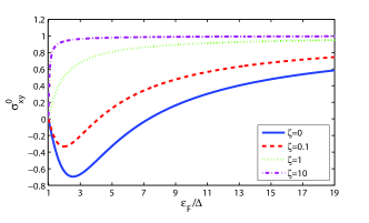
Figure 5: (color online). $\sigma^{0}_{xy}$ plotted as a function of the Fermi energy $\varepsilon_{F}$ for fixed values of $\zeta$. $\sigma^{0}_{xy}$ is measured in units of $e^{2}/(4\pi)$, and $\varepsilon_{F}$ is measured in units of $\Delta$.

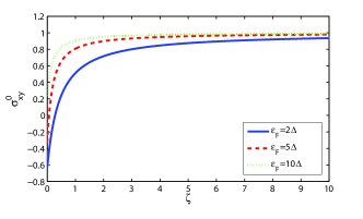
Figure 6: (color online). $\sigma^{0}_{xy}$ versus the ratio of scattering rates $\zeta$ for fixed values of Fermi energy $\varepsilon_{F}$. $\sigma^{0}_{xy}$ is measured in units of $e^{2}/(4\pi)$. The plot shows the crossover from Class A dominated regime to Class C dominated regime as $\zeta$ increases.

IV Discussion and Conclusion

As demonstrated in Sec.III, different scattering class has its own distinct contributions to AHE. This suggests that for the study of AHE in real materials, competing scattering processes belonging to different classes need to be handled carefully.

In ferromagnetic materials, normal (non-magnetic) impurity scattering and phonon scattering belong to Class A since they are isotropic in spin space. Most of the previous studies on extrinsic AHE are focused on this class of scattering and indeed it has been found that the electron-phonon scattering has similar contribution as normal impurity scattering (although there is no skew scattering due to conservation of phonon population in steady state),lyo1973 which is consistent with our theory. Magnetic impurities with spin directions oriented along the average magnetization is of Class B and they should generate a contribution different from that of normal impurities. This has also been observed in the study of dilute magnetic semiconductors. miha2008 ; nunn2008

Scattering processes of Class C also exist. For example, magnetic impurities with random in-plane magnetic orientation are of this class. Moreover the scattering of electron by magnons also belongs to Class C. To see this more clearly, let us consider the coupling between conduction electron spin $\bm{\sigma}$ and the local spin $\bm{S}$ (within an $s$-$d$ model approach),

$$\begin{split}\hat{H}_{\text{int}}&=-J\int d\bm{r}\left[\hat{\bm{\sigma}}(\bm{r})\cdot\bm{S}(\bm{r})\right]\\ &=-\frac{J}{2}\int d\bm{r}\left(\hat{\sigma}_{+}S_{-}+\hat{\sigma}_{-}S_{+}+2\hat{\sigma}_{z}S_{z}\right),\end{split}$$ (26)

where $J$ is the exchange coupling constant. The last term $2\hat{\sigma}_{z}S_{z}$ describes the Zeeman splitting (which has already been included in non-perturbed part of the Hamiltonian), whereas the first two terms describe the scattering by magnetic excitations. There is a transfer of spin angular momentum between conduction electrons and local spins during this process, hence such scattering is of Class C in our classification.

For real material samples that are studied experimentally, all the three classes of scattering are present at finite temperature. At low temperature, the scattering by normal impurity usually dominates. With increasing temperature, electron-magnon scattering becomes more important and can compete with normal impurity scattering and phonon scattering. Especially for materials with a high Debye temperature and a low Curie temperature, we can conceive a situation in which Class A and Class C scattering compete as depicted in Sec. III.F. Then the value of the side jump Hall conductivity would flow between the two limiting values as a function of temperature.

Finally we point out that the concept of “spin” in our discussion can be very general, corresponding to any discrete degrees of freedom (sometimes called a “pseudospin”). For example, in a bipartite lattice (such as graphene), the sublattice degree of freedom can be treated as pseudospin. Anomalous valley Hall transport occurs in graphene when there is sublattice symmetry breaking in the system. xiao2007 For bilayer systems, it is the layer index that plays the role of pseudospin. Then scattering processes can be classified according to their effects on the pseudospin. For example, inter-sublattice scattering in a bipartite lattice or interlayer scattering in a bilayer system would both belong to Class C. In general, our results indicate that a careful analysis of various scattering processes according to their pseudospin structures is indispensable for the study of AHE in these systems.

In summary, we have shown that the extrinsic part of the anomalous Hall conductivity has a strong dependence on the spin structure of the disorder scattering. We propose three universality classes of scattering according to their side jump contribution to the anomalous Hall conductivity. Each class has its distinct value of side jump. When two or more classes of scattering are competing, the side jump contribution is determined by their relative disorder strength. Various scattering processes in real physical systems can be classified into these three classes. In particular, we demonstrate that magnon scattering has distinct side jump contribution from normal impurity scattering and phonon scattering and the value of side jump contribution could change as system control parameter (such as temperature) varies.


Acknowlegement The authors thank N. A. Sinitsyn and J. Sinova for helpful discussions. H. Pan was supported by NSFC (10974011). Y. Yao was supported by NSFC (10974231) and the MOST Project of China (2007CB925000). Q. Niu was supported by DOE (DE-FG02-02ER45958 Division of Materials Science and Engineering) and Texas Advanced Research Program.

References

- (1) See N. Nagaosa, J. Sinova, S. Onoda, A. H. MacDonald, and N. P. Ong, Rev. Mod. Phys. 82, 1539 (2010) and references therein.
- (2) M. V. Berry, Proc. R. Soc. A 392, 45 (1984).
- (3) G. Sundaram and Q. Niu, Phys. Rev. B 59, 14915 (1999).
- (4) T. Jungwirth, Q. Niu, and A. H. MacDonald, Phys. Rev. Lett. 88, 207208 (2002).
- (5) M. Onoda and N. Nagaosa, J. Phys. Soc. Jpn. 71, 19 (2002).
- (6) J. Ye, Y. B. Kim, A. J. Mills, B. I. Shraiman, P. Majumdar, and Z. Tešanović, Phys. Rev. Lett. 83, 3737 (1999).
- (7) Taguchi, Y. Oohara, H. Yoshizawa, N. Nagaosa, and Y. Tokura, Science 291, 2573 (2001).
- (8) A. Crépieux and P. Bruno, Phys. Rev. B 64, 014416 (2001).
- (9) Z. Fang, N. Nagaosa, K. S. Takahashi, A. Asamitsu, R. Mathieu, T. Ogasawara, H. Yamada, M. Kawasaki, Y. Tokura, and K. Terakura, Science 302, 5642 (2003).
- (10) D. Culcer, A. H. MacDonald, and Q. Niu, Phys. Rev. B 68, 045327 (2003).
- (11) J. Schliemann and D. Loss, Phys. Rev. B 68, 165311 (2003).
- (12) J. Sinova, T. Jungwirth, and J. Černe, Int. J. Mod. Phys. B 18, 1083 (2004).
- (13) Y. Yao, L. Kleinman, A. H. MacDonald, J. Sinova, T. Jungwirth, D.-S. Wang, E. Wang, and Q. Niu, Phys. Rev. Lett. 92, 037204 (2004).
- (14) F. D. M. Haldane, Phys. Rev. Lett. 93, 206602 (2004).
- (15) W.-L. Lee, S. Watauchi, V. L. Miller, R. J. Cava, and N. P. Ong, Science 303, 1647 (2004).
- (16) N. A. Sinitsyn, Q. Niu, J. Sinova, and K. Nomura, Phys. Rev. B 72, 045346 (2005).
- (17) V. K. Dugaev, P. Bruno, M. Taillefumier, B. Canals, and C. Laroix, Phys. Rev. B 71, 224423 (2005).
- (18) J. Kötzler and W. Gil, Phys. Rev. B 72, 060412(R) (2005).
- (19) C. Zeng, Y. Yao, Q. Niu, and H. H. Weitering, Phys. Rev. Lett. 96, 037204 (2006).
- (20) S. Y. Liu, N. J. M. Horing, and X. L. Lei, Phys. Rev. B 74, 165316 (2006).
- (21) J.-I. Inoue, T. Kato, Y. Ishikawa, H. Itoh, G. E. W. Bauer, and L. W. Molenkamp, Phys. Rev. Lett. 97, 046604 (2006).
- (22) S. Onoda, N. Sugimoto, and N. Nagaosa, Phys. Rev. Lett. 97, 126602 (2006).
- (23) Y. Yao, Y. Liang, D. Xiao, Q. Niu, S.-Q. Shen, X. Dai, and Z. Fang, Phys. Rev. B 75, 020401(R) (2007).
- (24) N. A. Sinitsyn, A. H. MacDonald, T. Jungwirth, V. K. Dugaev, and J. Sinova, Phys. Rev. B 75, 045315 (2007).
- (25) M. F. Borunda, T. S. Nunner, T. Luck, N. A. Sinitsyn, C. Timm, J. Wunderlich, T. Jungwirth, A. H. MacDonald, and J. Sinova, Phys. Rev. Lett. 99, 066604 (2007).
- (26) T. Kato, Y. Ishikawa, H. Itoh, and J.-I. Inoue, New J. Phys. 9, 350 (2007).
- (27) T. S. Nunner, N. A. Sinitsyn, M. F. Borunda, V. K. Dugaev, A. A. Kovalev, Ar. Abanov, C. Timm, T. Jungwirth, J.-I. Inoue, A. H. MacDonald, and J. Sinova, Phys. Rev. B 76, 235312 (2007).
- (28) S. Y. Liu, N. J. M. Horing, and X. L. Lei, Phys. Rev. B 76, 195309 (2007).
- (29) N. A. Sinitsyn, J. Phys: Condens. Matter 20, 023201 (2008).
- (30) S. Onoda, N. Sugimoto, and N. Nagaosa, Phys. Rev. B 77, 165103 (2008).
- (31) T. S. Nunner, G. Zaránd, and F. von Oppen, Phys. Rev. Lett. 100 236602 (2008).
- (32) E. I. Rashba, Semiconductors 42, 905 (2008).
- (33) D. Venkateshvaran, W. Kaiser, A. Boger, M. Althammer, M. S. Ramachandra Rao, S. T. B. Goennenwein, M. Opel, and R. Gross, Phys. Rev. B 78, 092405 (2008).
- (34) L.-F. Arsenault and B. Movaghar, Phys. Rev. B 78, 214408 (2008).
- (35) A. A. Kovalev, Y. Tserkovnyak, K. Výborný, and J. Sinova, Phys. Rev. B 79, 195129 (2009).
- (36) S. Sangiao, L. Morellon, G. Simon, J. M. De Teresa, J. A. Pardo, J. Arbiol, and M. R. Ibarra, Phys. Rev. B 79, 014431 (2009).
- (37) Y. Shiomi, Y. Onose, and Y. Tokura, Phys. Rev. B 79, 100404(R) (2009)
- (38) M. Glunk, J. Daeubler, W. Schoch, R. Sauer, and W. Limmer, Phys. Rev. B 80, 125204 (2009).
- (39) Y. Tian, L. Ye, and X. Jin, Phys. Rev. Lett. 103, 087206 (2009).
- (40) A. A. Kovalev, J. Sinova, and Y. Tserkovnyak, Phys. Rev. Lett. 105, 036601 (2010).
- (41) D. Culcer, E. M. Hankiewicz, G. Vignale, and R. Winkler, Phys. Rev. B 81, 125332 (2010).
- (42) L. Berger, Phys. Rev. B 2, 4559 (1970).
- (43) The term which is proportional to need not vanish under the symmetry constraint. However, such scattering process is rearly physically relevant. Therefore in the interest of transparency we do not consider this term in the present work.
- (44) P. Středa, J. Phys. C 15, L717 (1982).
- (45) R. Karplus and J. M. Luttinger, Phys. Rev. 95, 1154 (1954).
- (46) For example, this contribution from Class B does not vanish for the -quadratic model .
- (47) Contribution to skew scattering involving disorder correlations higher than third order is conceivable. In our present model of scattering, we do not consider such correlations.
- (48) S.-K. Lyo, Phys. Rev. B 8, 1185 (1973).
- (49) G. Mihály, M. Csontos, S. Bordács, I. Kézsmárki, T. Wojtowicz, X. Liu, B. Jankó, and J. K. Furdyna, Phys. Rev. Lett. 100, 107201 (2008).
- (50) D. Xiao, W. Yao, and Q. Niu, Phys. Rev. Lett. 99, 236809 (2007).