Modeling large scale species abundance with latent spatial processes

Abstract

Modeling species abundance patterns using local environmental features is an important, current problem in ecology. The Cape Floristic Region (CFR) in South Africa is a global hot spot of diversity and endemism, and provides a rich class of species abundance data for such modeling. Here, we propose a multi-stage Bayesian hierarchical model for explaining species abundance over this region. Our model is specified at areal level, where the CFR is divided into roughly $37{,}000$ one minute grid cells; species abundance is observed at some locations within some cells. The abundance values are ordinally categorized. Environmental and soil-type factors, likely to influence the abundance pattern, are included in the model. We formulate the empirical abundance pattern as a degraded version of the potential pattern, with the degradation effect accomplished in two stages. First, we adjust for land use transformation and then we adjust for measurement error, hence misclassification error, to yield the observed abundance classifications. An important point in this analysis is that only $28\%$ of the grid cells have been sampled and that, for sampled grid cells, the number of sampled locations ranges from one to more than one hundred. Still, we are able to develop potential and transformed abundance surfaces over the entire region.

In the hierarchical framework, categorical abundance classifications are induced by continuous latent surfaces. The degradation model above is built on the latent scale. On this scale, an areal level spatial regression model was used for modeling the dependence of species abundance on the environmental factors. To capture anticipated similarity in abundance pattern among neighboring regions, spatial random effects with a conditionally autoregressive prior (CAR) were specified. Model fitting is through familiar Markov chain Monte Carlo methods. While models with CAR priors are usually efficiently fitted, even with large data sets, with our modeling and the large number of cells, run times became very long. So a novel parallelized computing strategy was developed to expedite fitting. The model was run for six different species. With categorical data, display of the resultant abundance patterns is a challenge and we offer several different views. The patterns are of importance on their own, comparatively across the region and across species, with implications for species competition and, more generally, for planning and conservation.

, , , and

T1Supported in part by NSF DEB Grants 056320 and 0516198.

1 Introduction

Ecologists increasingly use species distribution models to address theoretical and practical issues, including predicting the response of species to climate change [Midgley and Thuiller (2007), Fitzpatrick et al. (2008), Loarie et al. (2008)], designing and managing conservation areas [Pressey et al. (2007)], and finding additional populations of known species or closely related sibling species [Raxworthy et al. (2003), Guisan et al. (2006)]. In all these applications the core problem is to use information about where a species occurs and about relevant environmental factors to predict how likely the species is to be present or absent in unsampled locations.

The literature on species distribution modeling covers many applications; there are useful review papers that organize and compare model approaches [Guisan and Zimmerman (2000), Guisan and Thuiller (2005), Elith et al. (2006), Graham and Hijmans (2006), Wisz et al. (2008)]. Most species distribution models ignore spatial pattern and thus are based implicitly on two assumptions: (1) environmental factors are the primary determinants of species distributions and (2) species have reached or nearly reached equilibrium with these factors [Schwartz et al. (2006), Beale et al. (2007)]. These assumptions underlie the currently dominant species distribution modeling approaches—generalized linear and additive models (GLM and GAM), species envelope models such as BIOCLIM [Busby (1991)], and the maximum entropy-based approach MAXENT [Phillips and Dudík (2008)]. The statistics literature covers GLM and GAM models extensively. The latter tends to fit data better than the former since they employ additional parameters but lose simplicity in interpretation and risk overfitting and poor out-of-sample prediction. Climate envelope models and the now increasingly-used maximum entropy methods are algorithmic and not of direct interest here.

In addition to the fundamental ecological issues mentioned above, complication arises in various forms in modeling abundance from imperfect survey data such as observer error [Royle et al. (2007), Cressie et al. (2009)], variable sampling intensity, gaps in sampling, and spatial misalignment of distributional and environmental data [Gelfand et al. (2005a)]. First, since a region is almost never exhaustively sampled, individuals not exposed to sampling will be missed. Second, it may be that potentially present individuals are undetected [Royle et al. (2007)] and, possibly vice versa, for example, a false positive misclassification error with regard to species detection [Royle and Link (2006)]. A third complication is that ecologists and field workers are biased against absences; they tend to sample where species are, not where they aren’t. Such preferential sampling and its impact on inference is discussed in Diggle, Menezes and Su (2010). Further complications arise with animals due to their mobility. Previous work has developed spatial hierarchical models that accommodate some of these difficulties, fitting these models to presence/absence data in a Bayesian framework [Hooten, Larsen and Wikle (2003), Gelfand et al. (2005a, 2005b), Latimer et al. (2006)].

The species distribution modeling discussed above is either in the presence/absence or presence-only data settings; there is relatively little work on spatial abundance patterns, despite their theoretical and practical importance [Kunin, Hartley and Lennon (2000), Gaston (2003)]. Our primary contribution here is to develop a hierarchical modeling approach for ordinal categorical abundance data, explained by the suitability of the environment, the effect of land use/land transformation, and potential misclassification error. Ordinal classifications are often the case in ecological abundance data, especially for plants [Sutherland (2006), Ibáñez et al. (2009)]. From a stochastic modeling perspective, categorical data can be viewed as the outcome of a multinomial model, with the cell probabilities dependent on background features. Within a Bayesian framework such modeling is often implemented using data augmentation [Albert and Chib (1993)], introducing a latent hierarchical level. There, the ordered classification is viewed as a clipped version of a single latent continuous response, introducing cut points. See also De Oliveira (2000) and Higgs and Hoeting (2010).

At the latent level, suitability of the environment can be modeled through regression. Availability in terms of land use degrades suitability. That is, an important feature of our modeling, from an ecological point of view, is that it deals with transformation of the study area by human intervention. In much of the region, the “natural” state of areas has been altered to an agricultural or urban state, or the vegetation has been densely colonized by alien invasive plant species. So, we cannot treat the entire region as equally available to the plant species we are modeling. We must introduce a contrast between the current abundance of species (their transformed or adjusted abundance) and their potential distributions in the absence of land use change (potential abundance). These notions are formally defined at the areal unit level in Section 3. A further degradation enabling the possibility of misclassification and/or observer error in the data collection procedure can be accounted for as measurement error in the latent surface. There is a substantial literature on measurement error modeling for continuous observations, for example, Fuller (1987), Stefanski and Carroll (1987), and Mallick and Gelfand (1995). In our modeling we impose a hard constraint: with no potential presence (i.e., an unsuitable environment), we can observe only zero abundance. We enforce this constraint on the latent scale. With cut points, modeled as random, we provide an explanatory model for the observed categorical abundance data. Furthermore, we can invert from the latent abundance scale to the categorical abundances to predict abundance for unsampled cells and also to predict abundance in the absence of land use transformation.

With spatial data collection, we anticipate spatial pattern in abundance and thus introduce spatial structure into our modeling. That is, causal ecological explanations such as localized dispersal, as well as omitted (unobserved) explanatory variables with spatial pattern such as local smoothness of geological or topographic features, suggest that, at sufficiently high resolution, abundance of a species at one location will be associated with its abundance at neighboring locations [Ver Hoef et al. (2001)]. Moreover, through spatial modeling, we can provide spatial adjustment to cells that have not been sampled, accommodating the gaps in sampling and irregular sampling intensity mentioned above. In particular, we create a latent process model through a trivariate spatial process specification, with truncated support, to capture potential abundance, land transformation-adjusted abundance, and measurement error-adjusted abundance. Since our environmental information is available at grid cell level, we use Markov random field (MRF) models [Besag (1974), Banerjee, Carlin and Gelfand (2004)] to capture spatial dependence and to facilitate computation. However, we work with a large landscape of approximately $37{,}000$ grid cells which leads to very long run times in model fitting and so we introduce a novel parallelized computing strategy to expedite fitting.

There have been other recent developments in modeling of species abundances, some using Bayesian hierarchical models. First, there has been some work on developing models that deal almost exclusively with animal census data, including count data and mark-recapture data [Royle et al. (2007), Conroy et al. (2008), Gorresen et al. (2009)]. Potts and Elith (2006) provide an overview of abundance modeling, in fact, five regression models (Poisson, negative binomial, quasi-Poisson, the hurdle model, and the zero-inflated Poisson) fitted for one particular plant example. These models focus on correcting observer error and bias as well as under-detection (the species is present but not observed), whence the “true” abundance is virtually always higher than observed [Royle et al. (2007), Cressie et al. (2009)]. We note some very recent work on working with ordinal species abundance in plant data by Ibáñez et al. (2009). This approach takes ordinally scored abundances and uses an ordered logit hierarchical Bayes model to infer potential abundances for species that are still spreading across the landscape.

The advantages of working within the Bayesian framework with Markov chain Monte Carlo (MCMC) model fitting are familiar by now—full inference about arbitrary unknowns, that is, functions of model parameters and predictions, can be achieved through their posterior distributions, and uncertainty can be quantified exactly rather than through asymptotics. In this application we work with the disaggregated data at the level of individual species and sites to present spatially resolved abundance “surfaces” and to capture uncertainty in model parameters. Doing this turns out to be more difficult than might be expected, as we reveal in our model development section. The key modeling issues center on careful articulation of the definition of events and associated probabilities, the misalignment between the sampling for abundance (at the relatively small sampling sites) and the available environmental data layers (at a scale of minute by minute grid cells, roughly 1.55 km${}\times{}$1.85 km over the region), the sparseness of observations in terms of the entire landscape (with uneven sampling intensity including many “holes”), the occurrence of considerable human intervention with regard to land use across the landscape (“transformation”), and the need for spatially explicit modeling.

The format of the paper is as follows. Section 2 describes the motivating data set. Section 3 develops the multi-level abundance model. Section 4 details the computational and inference issues. In Section 5 we present an analysis of the data from the Cape Floristic Region (CFR) and conclude with some discussion and future extensions in Section 6.

2 Data description

The focal area for this abundance study is the Cape Floristic Kingdom or Region (CFR), the smallest of the world’s six floral kingdoms (Figure 1). As noted above, it encompasses a small region of southwestern South Africa, about 90,000 km², including the Cape of Good Hope, and is partitioned into 36,907 minute-by-minute grid cells of equal area. It has long been recognized for high levels of plant species diversity and endemism across all spatial scales. The region includes about 9000 plant species, $69\%$ of which are found nowhere else [Goldblatt and Manning (2000)]. Globally, this is one of the highest concentrations of endemic plant species in the world. It is as diverse as many of the world’s tropical rain forests and apparently has the highest density of globally endangered plant species [Rebelo (2002)]. The plant diversity in the CFR is concentrated in relatively few groups, such as the icon flowering plant family of South Africa, the Proteaceae. We focus on this family because the data on species distribution and abundance patterns are sufficiently rich and detailed to allow complex modeling. The Proteaceae have also shown a remarkable level of speciation, with about 400 species across Africa, of which 330 species are $99\%$ restricted to the CFR. Of those 330 species, at least 152 are listed as “threatened” with extinction by the International Union for the Conservation of Nature. Proteaceae have been unusually well sampled across the region by the Protea Atlas Project of the South African National Biodiversity Institute [Rebelo (2001)]. Data were collected at record localities: relatively uniform, geo-referenced areas typically 50 to 100 m in diameter. In addition to the presence (or absence) at the locality of protea species, abundance of each species along with selected environmental and species-level information were also tallied [Rebelo (1991)]. To date, some 60,000 localities have been recorded (including null sites), with a total of about 250,000 species counts from among some 375 proteas [Rebelo (2006)].

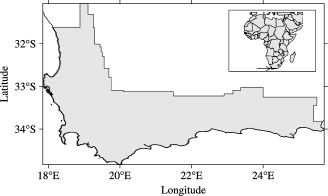
Figure 1: Location of the Cape Floristic Region (CFR) of South Africa. Inset shows the location of the CFR within the African Continent. The $90{,}000$ km² region was divided into $36{,}907$ $1$-minute cells for modeling.

Abundance is given for a sampling locality. Evidently, there is no notion of abundance at a point; however, with roughly $60{,}000$ sites sampled over the entire CFR, the relative scale of the Protea Atlas observations is small enough when compared to our areal units to be considered as “points.” In the literature, abundance is sometimes measured as percent cover [Mueller-Dombois and Ellenberg (2003)]. In our data set, abundance is recorded as an ordinal categorical classification of the count for the species with four categories: category 0$:$ none observed, category 1$:$ 1–10 observed, category 2$:$ 11–100 observed, category 3$:$ $>$100 observed. Such categorization is fast and efficient for studying many species and many sampling locations but is certainly at risk for measurement error in the form of misclassification. Additionally, a large number of cells were not sampled at all. In fact, only 10,158, that is, $28\%$, were sampled at one or more sites. Even among cells sampled, some have just one or two sites while others have more than 100, reflecting the irregular and opportunistic nature of the sampling rather than an experimentally designed sampling plan.

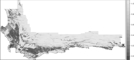
Figure 2: Proportion of untransformed land inside the CFR. Most of the transformation is due to agriculture, but includes dense stands of alien invasive species.

Turning to the covariates, in Gelfand et al. (2005a, 2005b) $16$ explanatory environmental variables were studied, capturing climate, soil, and topographic features (further detail is provided there). Here, we confine ourselves to the six most significant variables from that study, which are Evapotranspiration (APAN.MEAN), July (winter) minimum temperature (MIN07), January (summer) maximum temperature (MAX01), mean annual precipitation (MEAN.AN.PR), summer soil moisture days (SUMSMD), and soil fertility (FERT1). Transformed areas (by agriculture, reforestation, alien plant infestation, and urbanization) were obtained as a GIS data layer from R. Cowling (private communication). Figure 2 shows the pattern of transformation across the CFR. Approximately $1/3$ of the Cape has been transformed, mainly in the lowlands on more fertile soils where rainfall is adequate [Rouget et al. (2003)]. Most of the transformation outside of these areas, on the infertile mountains, is due to dense alien invader species, which are currently a major threat to Fynbos vegetation and, in particular, to the Proteaceae.

3 Multi-level latent abundance modeling

In Section 3.1 we briefly review the earlier work on hierarchical modeling for presence/absence data, presented in Gelfand et al. (2005a, 2005b), in order to reveal how we have generalized it for the abundance problem. Section 3.2 develops our proposed probability model for the categorical abundance data. In Section 3.3 discrete probability distributions are replaced using latent continuous variables. In Section 3.4 we discuss bias issues associated with modeling abundance data and, in particular, how they affect our setting. Section 3.5 deals with explicit model details for the likelihood and posterior.

3.1 Hierarchical presence/absence modeling

In Gelfand et al. (2005a,2005b) the authors model at the scale of the grid cells in the CFR and provide a block averaged binary process presence/absence model at this scale. In particular, let $A_{i}\subset\mathbb{R}^{2}$ denote the geographical region corresponding to the $i$th grid cell and $X_{i}^{(k)}$ the event that a randomly selected location within $A_{i}$ is suitable (1) or unsuitable (0) for species $k$. Set $P(X_{i}^{(k)}=1)=p_{i}^{(k)}$. Then, $p_{i}^{(k)}$ is conceptualized by letting $\lambda^{(k)}(s)$ be a binary process over the region indicating the suitability (1) or not (0) of location $s$ for species $k$ and taking $p_{i}^{(k)}$ to be the block average of this process over unit $i$. That is,

$$p_{i}^{(k)}=\frac{1}{|A_{i}|}\int_{A_{i}}\lambda^{(k)}(s)\,ds=\frac{1}{|A_{i}|}\int_{A_{i}}\mathbf{1}\bigl{(}\lambda^{(k)}(s)=1\bigr{)}\,ds,$$ (1)

where $|A_{i}|$ denotes the area of $A_{i}$. From Equation (1), the interpretation is that the more locations within $A_{i}$ with $\lambda^{(k)}(s)=1$, the more suitable $A_{i}$ is for species $k$, that is, the greater the chance of potential presence in $A_{i}$. The collection of $p_{i}^{(k)}$’s over the $A_{i}$ is viewed as the potential distribution of species $k$.

Let $V_{i}^{(k)}$ denote the event that a randomly selected location in $A_{i}$ is suitable for species $k$ in the presence of transformation of the landscape. Let $T(s)$ be an indicator process indicating whether location $s$ is transformed ($1$) or not (0). Then, at $s$, both $T(s)=0$ (availability) and $\lambda^{(k)}(s)=1$ (suitability) are needed in order that location $s$ is suitable under transformation. Therefore,

$$P\bigl{(}V_{i}^{(k)}=1\bigr{)}=\frac{1}{|A_{i}|}\int_{A_{i}}\mathbf{1}\bigl{(}T(s)=0\bigr{)}\mathbf{1}\bigl{(}\lambda^{(k)}(s)=1\bigr{)}\,ds.$$ (2)

If, for each pixel, availability is uncorrelated with suitability, then Equation (2) simplifies to $P(V_{i}^{(k)}=1)=u_{i}p_{i}^{(k)}$, where $u_{i}$ denotes the proportion of area in $A_{i}$ which is untransformed, $0\leq u_{i}\leq 1$.

Next, assume that $A_{i}$ has been visited $n_{i}$ times in untransformed areas within the cell. Further, let $y_{ij}^{(k)}$ be the observed presence/absence status of the $k$th species at the $j$th sampling location within the $i$th unit. The $y_{ij}^{(k)}|V_{i}^{(k)}=1$ are modeled as i.i.d. Bernoulli trials with success probability $q_{i}^{(k)}$, that is, for a randomly selected location in $A_{i}$, $q_{i}^{(k)}$ is the probability of species $k$ being present given the location is both suitable and available. Of course, given $V_{i}{(k)}=0$, $y_{ij}^{(k)}=0$ with probability 1. Then, we have that $P(y_{ij}^{(k)}=1)=q_{i}^{(k)}u_{i}p_{i}^{(k)}$. Gelfand et al. (2005a, 2005b) model the $p_{i}^{(k)}$ and $q_{i}^{(k)}$ using logistic regressions. In fact, they use environmental variables and spatial random effects to model the $p_{i}^{(k)}$’s, the probabilities of potential presence, and, to facilitate identifiability of parameters, use species level attributes to model the $q_{i}^{(k)}$’s.

3.2 Probability model for categorical abundance

We first define what categorical abundance means at an areal scale using the four ordinal categories from Section 2. Suppressing the species index, let $X_{i}$ denote the classification for a randomly selected location in $A_{i}$ and define $p_{ih}$ $=$ $P(X_{i}=h)$ for $h=0,1,2,3$. If $\lambda(s)$ is a four-colored process taking values $0,1,2,3$, then $p_{ih}=\frac{1}{|A_{i}|}\int_{A_{i}}1(\lambda(s)=h)\,ds$. That is, $p_{ih}$ is the proportion of area within $A_{i}$ with color $h$, equivalently, the proportion in abundance class $h$. The $p_{ih}$ denote the potential abundance probabilities, that is, in the absence of transformation.

We describe land transformation percentage $(1-u_{i})$ as a block average of a binary availability process $T(s)$ over $A_{i}$. It can also be interpreted as the probability that a randomly selected site within $A_{i}$ is transformed. At a transformed location abundance must be $0$. Thus, as in Equation (2), in the presence of transformation, we revise $p_{ih}$ to $P_{T}(X_{i}=h)=\frac{1}{|A_{i}|}\int_{A_{i}}1(T(s)=0)1(\lambda(s)=h)\,ds$. Under independence of abundance and land transformation, we obtain $P_{T}(X_{i}=h)=u_{i}p_{ih}$. The $u_{i}p_{ih}$ denote the transformed abundance probabilities for $h\neq 0$. The probability of abundance class $0$ under transformation is evidently $1-u_{i}+u_{i}p_{i0}$. Let $r_{ih}$ denote the abundance class probabilities in the presence of transformation.

Finally, suppose there is an observed categorical abundance at location $j$ within $A_{i}$, say, $y_{ij}$. There is an associated conceptual $\lambda_{ij}$ and an observed $T_{ij}$. Then, $\lambda_{ij}\neq\lambda_{ij}T_{ij}$ if there has been transformation degradation at location $j$, unless $\lambda_{ij}=0$. Furthermore, if there has been a misclassification error at $j$, $y_{ij}\neq\lambda_{ij}T_{ij}$ unless $\lambda_{ij}=0$. Let $q_{ih}$ denote the abundance class probabilities associated with the observed abundances. In Section 3.3 we specify a latent trivariate continuous abundance model that produces the $p$’s, $r$’s, and $q$’s by integrating over appropriate intervals. This latent model can be viewed as the process model for our setting.

The data set consists of observed abundances across several sampling sites within the CFR. Let $D$ denote our CFR study domain so $D$ is divided into $I=36{,}907$ grid cells of equal area. For each cell $i=1,2,3,\ldots,I$, we are given information on $p$ covariates as $v_{i}=(v_{i1},v_{i2},\ldots,v_{ip})$. Within $A_{i}$, the abundance category of a species was recorded at each of $n_{i}$ sampling sites. For many cells $n_{i}>1$. For site $j$ in $A_{i}$ we observe $y_{ij}$ as a multinomial trial, that is, $y_{ij}\stackrel{{\scriptstyle\mathrm{i.i.d.}}}{{\sim}}\operatorname{mult}(\{q_{ih}\}),j=1,2,\ldots,n_{i}$. We have a large number of unsampled cells, that is, $n_{i}=0$. In fact, out of 36,907 cells, only $m=10{,}158$ ($28\%$) were sampled at one or more sites. Figure 3 indicates locations of sampled cells. For the unsampled cells there are no $y_{ij}$’s in the data set. Hence, the inference problem involves estimation of probabilities over the observed cells as well as prediction over the unsampled region. Prediction of a categorical response distribution for unsampled locations in a point level model was discussed in De Oliveira (2000) and Higgs and Hoeting (2010). In our areal setup with only areal level $v$’s, we address this problem with a MRF model, as described in Section 3.3. Again, we seek to infer about the $p$’s, $r$’s, and $q$’s given the observed $y$’s for a subset of cells and $v$’s known for all cells.

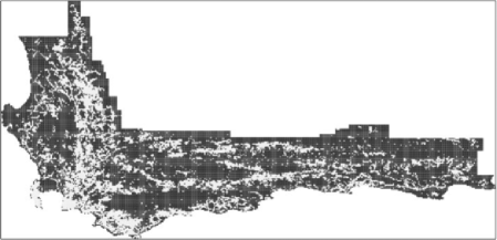
Figure 3: Cells within the CFR that have at least one observation from the Protea Atlas data set are shown in light grey, while cells with no observations are shown in dark grey.

3.3 Latent continuous abundances

It is now common to model the probability mass function of a scalar ordinal categorical variable through an underlying univariate continuous distribution. In a more general setup, Le Loc’h and Galli (1997) and Armstrong et al. (2003) used latent random vectors to define the categorical probabilities in terms of these vectors taking values within a specific set. In a similar spirit, corresponding to an observed abundance category variable $y_{ij}$, we introduce a continuous latent variable $z_{O,ij}$ such that

$$y_{ij}=\sum_{h=0}^{3}h1(\alpha_{h-1}<z_{ij}<\alpha_{h}),$$

where $\alpha=(\alpha_{-1}=-\infty,\alpha_{0}=0,\alpha_{1},\alpha_{2},\alpha_{3}=\infty)$ are an increasing sequence of cut points. For identifiability and without loss of generality, we can set $\alpha_{0}=0$ and interpret $z_{O,ij}<0$ as an absence, $z_{O,ij}>0$ as a presence. We have $P(y_{ij}=h)=q_{ih}=P(z_{O,ij}\in(\alpha_{h-1},\alpha_{h}))$. So $q_{ih}$ will be determined by the probability model specified for the $z_{O,ij}$’s. We will introduce spatial dependence between $z_{O,ij}$’s below but, for now, to simplify notation, we drop the subscript.

A simple model would put a Gaussian distribution on these latent $z_{O}$’s whose means are linear functions of the associated $v$’s. This would provide a routine categorical regression model but ignores known land transformation and potential measurement/ecological error in the recorded abundance categories. Instead, we introduce $z_{P,ij}$ to provide the $p_{ij}$’s and $z_{T,ij}$ to provide the $r_{ij}$’s. We need a joint distribution to relate the $z_{P}$, $z_{T}$, and $z_{O}$. From a process perspective in terms of the proposed degradation, it seems natural to specify this distribution in the form $f(z_{P})f(z_{T}|z_{P})f(z_{O}|z_{T})$. Since ($z_{P},z_{T},z_{O}$) capture the sequential degradation of an associated categorical abundance distribution, we need to use the same set of $\alpha$’s to produce meaningful ($p,r,q$) respectively. Now, we propose (and clarify) the following dependence structure. Define $c(\mu)=\mu-\frac{\phi(\mu)}{\bar{\Phi}(\mu)}$, where $\phi(\cdot)$ and $\Phi(\cdot)$ are the standard normal p.d.f. and c.d.f. respectively. Note that $c(\mu)=E(V|V\sim N(\mu,1),V<0)$ so $c(\mu)\leq\min(0,\mu)$ for all $\mu\in\mathbb{R}$. Let

$$P(y=h|z_{O},u) = 1({\alpha_{h-1}\leq z_{O}\leq\alpha_{h}});\qquad 0\leq h\leq 3,$$

$$f(z_{O}|z_{T}) = \phi(z_{O};z_{T},1)1_{z_{T}\geq 0}+\delta_{z_{T}}1_{z_{T}\leq 0},$$

$$f(z_{T}|z_{P},u) \sim u\delta_{z_{P}}+(1-u)\delta_{c(z_{P})},$$

$$f(z_{P}|v,\beta,\tau^{2}) = \phi(z_{P};v^{T}\beta+\theta,1).$$

Again, the conditional modeling above is motivated by the degradation perspective. To model the latent $z_{P}$ surface, we use the covariate information, that is, climate and soil features that are believed to influence the abundance distribution of different species in different ways. We also add a spatial random effect ($\theta$) in the mean function to account for spatial association that may arise from factors, apart from included covariates, that may have a spatial pattern. The covariate effects $\beta$ as well as the spatial random effects $\theta$ are species-specific. Variances are fixed at 1 for identifiability (see Section 3.5). Since we are working at areal scale, we assign each cell a single $\theta$ with the prior on $\theta_{1,2,\ldots,I}$ specified using a Gaussian Markov random field (MRF) [Besag (1974)] with first-order adjacency proximities. See Banerjee, Carlin and Gelfand (2004) for details as well as further references.

Next, the $z_{P}$ surface is degraded by land transformation. A random location inside $A_{i}$ is untransformed with probability $u_{i}$. Then, $z_{T}=z_{P}$, that is, a degenerate distribution at $z_{P}$ given $z_{P}$. If it is transformed, the degradation occurs so that the $z_{T}$ corresponds to the zero abundance category. For simplicity (with further discussion below), we make this a degenerate distribution at $c(z_{P})<0$, whence $z_{T}|z_{P},u$ becomes a two point distribution as above. Again, transformation is equivalent to absence and since $\alpha_{0}=0$ is the upper threshold for that classification, we need $z_{T}<0$ for a transformed location. When a cell is completely transformed, from Equation (3.3) we have $z_{T}<0$ w.p. $1$. For $u=1$ (complete availability) $z_{T}$ and $z_{P}$ are the same. For any $0<u<1$, we get $E(z_{T}|z_{P})=uz_{P}+(1-u)c(z_{P}).$

Also, since $c(x)<x$, $E(z_{T}|z_{P})\leq z_{P}$, which is essential in the sense that transformation can only degrade abundance [and clarifies our choice for $c(\cdot)$]. Posterior summaries of $z_{T}$ measure the prevailing abundance under transformation within the CFR. [In Appendix .1 we show that $|E(z_{T})|<\infty$.] The two-point mixture distribution also implies the probability of abundance class $0$, $P(z_{T}<0)\geq(1-u)$, that is, no matter how large the potential abundance is within a cell, for any $u<1$ there is a positive probability that transformed abundance may fall below $0$ at a random location within the cell. Other choices for the $z_{T}|z_{P}$ specification besides a point mass at $c(z_{P})$ include putting a point mass at some arbitrary point $c<0$, or using a truncated normal $z_{T}|z_{P}$ on $\mathbb{R}^{-}$. In the first case, it is not ensured whether $z_{T}\leq z_{P}$ (it depends on whether there are cells with $z_{P}<c$), while the second choice adds complication for no benefit, is less interpretable, and does not ensure $z_{T}<z_{P}$ with probability $1$. Also, in Section 4 we show that, in terms of fitting the model, the specification used in Equation (3.3) is the same as using a truncated normal distribution for land transformation.

Next, we modify the {$z_{T}$} surface to produce {$z_{O}$}. With regard to measurement error, the recorded category of abundance at a particular location can be different from the prevailing category due to inaccuracy in field assessment of species quantity. However, we assume that when the potential abundance was zero, one could not record a nonzero abundance category for it [no false positives, see Royle and Link (2006) in this regard]. This puts a directional constraint on the effect of noise. A specification for $f(z_{T}|z_{O})$ which is coherent with this restriction has, with $z_{T}>0$ (i.e., a presence), $z_{O}|z_{T}\sim N(z_{T},1)$. This is a usual measurement error model (MEM) specification. For a site with no presence $z_{T}<0$, our assumption says there cannot be any measurement error, thus, in Equation (3.3), for simplicity, we set $z_{O}$ to be the same as $z_{T}$. Again, other choices of $z_{O}|z_{T}$ can be considered for the $z_{T}<0$ event, but they will not have any impact on estimation of the $z_{P}$ surface, as we clarify in Section 4. This sequential dependence structure, $z_{P}\rightarrow z_{T}\rightarrow z_{O}$, implies that if $z_{P}<0$ so is $z_{T}$ and $z_{O}$. Hence, if a site is not suitable for a species, at no intermediate stage of the model can the site have any positive probability of species occurrence. A change in category between actual and observed arises when the noise pushes $z_{T}$ to the other side of some cut point to produce $z_{O}$. And, because of the truncation structure, that shift cannot happen from the left of $\alpha_{0}=0$ to the right.

An alternative way to jointly model $(z_{O},z_{T})$ could use a bivariate normal distribution with support truncated to $\mathbb{R}^{2}-[0,\infty)\times(-\infty,0]$. However, this specification fails to produce an $f(z_{O}|z_{T})$ which match our intuition about how the degradation took place. Also, from the distributional perspective, the truncated normal redistributes the mass contained inside the left-out region uniformly across the support, whereas the specification in Equation (3.3) shifts the mass only to $(z_{O}<0)$, which is more in agreement with modeling a data set such as ours where we have an inflated number of reported zero abundances.

The simple dependence structure for $z_{T}|z_{P}$ allows us to marginalize over $z_{T}$ and work with $z_{P}$ and $z_{O}|z_{P}$ as our joint latent distribution. We have

$$f(z_{O}|z_{P})=\cases{u\phi(z_{O};z_{P},1)+(1-u)\delta_{c(z_{P})},&\quad$z_{P}>0$,\cr u\delta_{z_{P}}+(1-u)\delta_{c(z_{P})},&\quad$z_{P}<0$.}$$ (4)

Rewriting Equation (4) in a simpler form, we get

$$f(z_{O}|z_{P}) \sim u[\phi(z_{O};z_{P},1)1_{z_{P}\geq 0}+\delta_{z_{P}}1_{z_{P}\leq 0}]+(1-u)\delta_{c(z_{P})}.$$ (5)

Moreover, Equation (5) has a nice interpretation in the sense that, first, it indicates whether the land is transformed or not with probability $1-u$. If the land is transformed, it sets observed abundance to be $z_{O}=c(z_{P})<z_{P}$. In the case of available land, if there is a potential presence, it allows for a MEM around $z_{P}$; in the case of absence, it stays fixed at $z_{P}$. Since $z_{O}$ is related to the observed data and $z_{P}$ is our surface of interest, the marginalization removes one stage of hierarchy from our model fitting and thus reduces correlation, yielding better behaved MCMC in model fitting. Furthermore, we can retrieve the $z_{T}$ surface after the fact since $f(z_{T}|z_{O},z_{P})\propto f(z_{T}|z_{P})f(z_{O}|z_{T})$.

3.4 Measurement error and bias issues

In the Introduction we noted that measurement error and bias typically occur with ecological survey data. It can manifest itself in the form of detection error, spatial coverage bias [Royle et al. (2007)], and under-reporting of absences. How do these biases arise in our modeling? Noteworthy points here are (i) the difference between obtaining abundance as actual counts as opposed to through ordinal classifications and (ii) what “no abundance” means across our collection of grid cells.

Nondetection bias (i.e., undetected individuals in a sampled location) tends to be discussed more with regard to animal abundance [Ver Hoef and Frost (2003), Royle et al. (2007), Gorresen et al. (2009)]. Using counts, evidently observed abundance is at most true abundance; error can occur in only one direction. With ordinal counts, the bias is still expected to reflect under-reporting but, depending upon the categorical definitions, will be much less frequent and need not be absolutely so. For example, in our data set, plant population size is visually estimated and an observation, especially of large populations, could potentially have error in either direction. In our modeling, “true” abundance is not “potential” abundance. For us, one could envision true abundance on the latent scale as a “true” transformed abundance, say, $\tilde{z}_{T}$ with measurement error yielding $z_{O}$. Then, one might insist that our measurement error model requires $z_{O}\leq\tilde{z}_{T}$. Under our measurement error formulation using $z_{T}$, we even allow $z_{O}>z_{P}$ to account for potential overestimation of abundance. Evidently, since $y_{O}$ may occasionally be less than the potential classification $y_{P}$ at that location, we may be slightly underestimating potential abundance. We don’t expect this to be consequential and, in any event, with no knowledge about the incidence of under-classification in our setting, we have no sensible way to correct for this bias.

Turning to spatial coverage bias (i.e., individuals not exposed to sampling will be missed), for us, with only $28\%$ of grid cells sampled, we certainly are subject to this. However, the spatial modeling we introduce helps in this regard. The mean of $z_{P,ij}$ is $v_{i}^{T}\beta+\theta_{i}$ regardless of whether we collected any data in $A_{i}$. So, the regression is expected to find the appropriate level for the cell and the spatial smoothing associated with the $\theta_{i}$ is expected to provide suitable local adjustment. We could argue that, if sampling of grid cells is random, this bias can be ignored.

Perhaps the most difficult bias to address is the under-sampling of absences. This bias counters the previous ones; under-sampling of absences will tend to produce over-estimates of potential abundance. In our setting, under-sampling of absences is reflected in the decision-making that leads to only $28\%$ of cells being sampled, that is, it is not a random $28\%$ that have been sampled. Different from spatial coverage bias, in this context, the ecologist expresses confidence that the species is not present in some of the unsampled cells. If this is so and we were to set some additional abundances to $0$, this would assert that these “0”s are not nondetects and would diminish potential abundance, opposite to the case of nondetects. Of course, in the absence of actual data collection, we would not see any of these $0$’s and would adopt model-based inference regarding potential abundance for these cells. In any event, with no explicit knowledge of how sampling sites were chosen, we are unable to attempt correction for this bias. Possibly, approaches to address the effects of preferential sampling [Diggle, Menezes and Su (2010)] could be attempted here.

3.5 Likelihood and posterior distribution

The posterior distributions of interest, $p$ and $r$, will be constructed in the post MCMC analysis (discussed in detail in Section 4.3). From the conditional structure we first write $P(y=c|z_{O},\alpha)=1_{z_{O}\in(\alpha_{c-1},\alpha_{c})}$. So the likelihood function for a single sample $y$ turns out to be $L(y|z_{O},\alpha)=\prod_{k=0}^{3}1({z_{O}\in(\alpha_{k-1},\alpha_{k})})^{1(y=k)}$. Now $f(z_{O}|z_{P})$ can be written as in Equation (5).

Again, we have $I$ cells with $n_{i}$ sampling sites within $A_{i}$. For each $y_{ij}$ we introduce a corresponding $z_{O,ij,}$ and hence a pair of $z_{T,ij},z_{P,ij}$, to represent the event happening at the $j$th sampling site within $A_{i}$. We work directly with the $z_{O}|z_{P}$ structure. Since we are interested in the areal level abundance distribution and have covariates at areal resolution, we assume for fixed $i$, $z_{P,ij}$ $\stackrel{{\scriptstyle\mathrm{i.i.d.}}}{{\sim}}$ $N(\cdot;v_{i}^{T}\beta+\theta_{i},1)$. It is also assumed that the $z_{O,ij}$’s are conditionally independent given the $z_{P,ij}$’s.

Without loss of generality, re-index cells so that the first $m$ of them are sampled and the last $I-m$ are not. The latter cells have no contribution to the $y$ column and, hence, no associated $z_{O}$ appears in the likelihood. Using a nonspatial model, we would work with a posterior on the domain of sampled cells only. But assuming a CAR prior structure with adjacency proximity matrix $W$ for the $\theta$ over the whole domain enables us to learn about $z_{P}$ for unsampled cells. In summary, the posterior distribution takes the following form, up to proportionality, with $\Theta=(\bolds{\alpha},\bolds{\beta},\bolds{\theta})$:

$$\hskip 35.0pt\pi(\mathbf{z}_{P},\mathbf{z}_{O},\Theta|\mathbf{y,v,u}) \propto \prod_{i=1}^{m}\prod_{j=1}^{n_{i}}L(y_{ij}|z_{O,ij},\bolds{\alpha})f(z_{O,ij}|z_{P,ij})f(z_{P,ij}|v_{i},\Theta)$$

$${}\times\pi(\Theta),$$

$$\pi(\Theta) = \pi(\bolds{\alpha})\pi(\bolds{\beta})\pi(\bolds{\theta}),$$

$$\pi(\theta_{1,2,\ldots,I}) = \operatorname{CAR}(\eta_{0},W).$$

We turn to the identifiability of the set of parameters under the hierarchical dependent latent structure. First, with a latent continuous process yielding an ordinal categorical variable, the mean and scale of the distribution can be identified only up to their ratio. In Equation (3.3) the dependence across $(z_{p},z_{T},z_{O})$ is specified through conditional means. Hence, all Gaussian distributions there are specified with standard deviation $1$. Four categories of abundance allow three free probabilities and the corresponding four latent surfaces will also have $3$ degrees of freedom. As noted above, we set $\alpha_{0}=0$ with $\alpha_{1},\alpha_{2}$ as free parameters.

We also need to ensure that all three $z$ surfaces can be distinguished from each other. Since transformation percentage $1-u$ is given a priori, it is straightforward to separate $z_{P}$ and $z_{T}$. We turn to the joint distribution for $z_{P},z_{O}$ given as $z_{O}|z_{P}\sim N(z_{P},1),z_{P}\sim N(v\beta+\theta,1)$. With fixed variances and no constraint on measurement error, there would be no need to bring in $z_{P}$; it is redundant, there is no way to distinguish between $z_{P}$ and $z_{O}$, and one can use the marginal $z_{O}\sim N(v\beta+\theta,2)$. Now the constraint comes into the picture; it makes the $z_{O}$ surface non-Gaussian though the $z_{P}$ surface is. The greater the measurement error, the more departure from Gaussianity in the marginal distribution of $z_{O}$. Again, the measurement error cannot be estimated on any absolute scale, since the latent $z$ scales are fixed for identifiability. It will be controlled by parameters like $\beta$ and $\theta$. To compare the relative effect of measurement error across different species, under fixed scale parameters, $P(z_{P}<0)$ is a candidate but other model features can be informative as well.

Finally, the full model specification, described in Equation (3.3), can be represented through a graphical model, shown in Figure 4.

Figure 4: Graphical model for latent abundance specification at site $j$ within cell $A_{i}$. $z$’s denote latent abundance processes, observed (O), transformed (T), and potential (P); $y$’s denote interval-censored abundances, observed (O), and potential (P); $u$ is proportion of land untransformed, $v$’s are covariates, $\beta$’s are regression coefficients, $\alpha$’s are cut points for $z$ scale, and $\theta$’s are spatial random effects.

4 Posterior computation and inference

Here, we describe how to design a computationally efficient MCMC algorithm for the model. We then discuss how to summarize the posterior samples to estimate important model features.

4.1 Sampling

Introduction of latent layers, although increasing the parameter dimension in the model, makes the posterior full conditionals standard and easy to sample from. Our goal is to efficiently estimate components of $\Theta$ which control potential abundance. We rewrite Equation (5) as follows:

$$f(z_{O}|z_{P}) = u\phi(z_{O};z_{P},1)1_{z_{P}\geq 0}+\bigl{[}u\delta_{z_{P}}+(1-u)\delta_{c(z_{P})}\bigr{]}1_{z_{P}\leq 0}$$

$${}+(1-u)\delta_{c(z_{P})}1_{z_{P}>0},$$

and work with Equation (4.1) to implement the computation for the model fitting.

We start with updating all $z_{O},z_{P}$ using $(\Theta^{(t)};\mathbf{y,v,u})$ and then drawing components of $\Theta$ from their respective posterior full conditionals based on $z_{P,(t+1)},$ $z_{O,(t+1)}$. Given the draw from $z_{P}$, sampling the components of $\Theta$ is standard as in almost any spatial regression analysis (see Appendix .3). For the set of $\theta$’s, after sampling them sequentially, we need to “center them on the fly” [Besag and Kooperberg (1995), Gelfand and Sahu (1999)]. The more challenging part is to update $z_{O},z_{P}|\Theta$. In Albert and Chib (1993) the latent variables were sampled in the MCMC from mutually independent truncated Gaussian full conditionals, with the support determined by the corresponding classification. For our model, the posterior full conditional for any $z_{O}$ is

$$\pi(z_{O}|z_{P},y,u)\propto f(z_{O}|z_{P})1\bigl{(}{z_{O}\in(\alpha_{y-1},\alpha_{y})}\bigr{)}.$$

We take two different strategies to update $z_{P},z_{O}$ depending on the observed $y$. For any site with nonzero $y$ we have (with $\alpha_{0}=0$) $f(z_{O},z_{P}|y>0,u)\propto\phi(z_{O}|z_{P})1_{z_{O}\in(\alpha_{y-1},\alpha_{y})}\phi(z_{P})$, which amounts to sampling first a univariate normal $z_{O,(t+1)}|(z_{P,(t)},y,\alpha)$ truncated within $(\alpha_{y-1}^{(t)},\alpha_{y}^{(t)})$ and then from $z_{P,(t+1)}|$ $z_{O,(t+1)},\Theta^{(t)}$ which is also Gaussian [with location $(z_{O,(t+1)}+{\mu}^{(t)})/2$ and scale $\sqrt{1/2}$ where $\mu^{(t)}=v^{T}\beta^{(t)}+\theta^{(t)}]$. For a site with observed $y=0$ the case is more complicated, with details provided in Appendix .2. All of the sampling distributions required in MCMC are listed in Appendix .3.

4.2 Computational efficiency

The algorithm described above is computationally demanding as we have two latent variables to sample at each sampling site and one spatial parameter for each of the grid cells. However, since $z_{P},z_{O}$ are independent across cells given $\Theta$, we can update them all at once. The problematic part is sampling the spatial effects, with approximately 37,000 grid cells. To handle this issue, we used a parallelization method where $D$ is divided into disjoint and exhaustive subregions $D_{1},D_{2},\ldots,D_{L}$ along with a resultant set of boundary cells $B$ arising through the CAR proximity matrix. Thus, once $\theta_{B}$ is updated conditional on the rest, then $\theta_{D_{1}},\theta_{D_{2}},\ldots,\theta_{D_{L}}$ given $\theta_{B}$ can be updated in parallel.

This algorithm is illustrated in Figure 5, where we have a $15\times 8$ rectangular region with an adjacency structure $W$ which puts weight only on the cells sharing a common boundary. Sequential updating would have required $120$ steps. We constructed a set of $48$ boundary cells $B$ (the dark cells in Figure 5). It divides the rectangle into $12$ segments of $6$ cells each, so that conditional on $\theta_{B}$, those segments can be updated independently of each other so we need only $54$ updating steps. This is only an illustrative example, but for large regions, this may significantly improve the run time. However, the time required for communication and data assimilation is an issue for this parallelization method. With increasing $L$, although the time required for the sequential updating within each $D_{i}$ goes down, the size of $B$ increases as does the amount of communication required within the parallel architecture. So a trade-off must be determined for choosing $L$; in our setting $L=11$ worked well.

Figure 5: An example grid to illustrate parallel CAR implementation. Normal sequential updating would have required $120$ steps in each iteration. By dividing the rectangle into $12$ segments of $6$ cells each with $48$ boundary cells (shown in dark grey), each segment can be updated independently (conditional on the boundaries). In this example the parallelization results in only $54$ updating steps.

4.3 Posterior summaries

There are several ways to summarize inference about the $p$ and $r$ distributions. According to our model, for $A_{i}$, $p_{ih}=\Phi(\alpha_{h}-v_{i}^{T}\beta-\theta_{i})-\Phi(\alpha_{h-1}-v_{i}^{T}\beta-\theta_{i})$. Posterior samples of $\beta,\theta,\tau^{2}$ enable us to compute samples of the $p_{i}$. A posterior sample of $r_{i}$ can be constructed using the relation $r_{i}\equiv(1-u_{i}+u_{i}p_{io},u_{i}p_{i1},u_{i}p_{i2},u_{i}p_{i3})$. Additionally, we can calculate the mean as well as the uncertainty from these samples, enabling maps for transformed abundance ($r$) and potential ($p$) abundance. For each of $p_{i}$ and $r_{i}$, we have $4$ submaps, one for each abundance category. This is useful in terms of assessing high and low abundance regions for the species. The $\beta$’s provide (up to fixed scale) the effect of a particular climate or soil-related factor on the abundance of a particular species. Comparison of the $p$ and $r$ maps informs about the effect of land transformation. One may also be interested in capturing $p$ or $r$ through a single summary feature rather than all $4$ categorical probabilities. Grouped mean abundance (expectation with respect to the $p$ or $r$ distribution) can be used with suitable categorical midpoints. We note that the posterior inference can also be summarized on the latent scale using posterior samples of the $z$’s. However, working on the $z$ scale can only provide relative comparison.

5 Data analysis

Table 1: Posterior summaries for covariate effects (mean and $95$% c.i. width)

Species	Apan.mean	Max$\bolds{01}$	Min$\bolds{07}$	Mean.an.pr	Sumsmd	Fert$\bolds{1}$
PRPUNC	$1.2275$	$-0.9436$	$-0.8248$	$0.2439$	$0.1834$	$0.0306$
	$(0.3809)$	$(0.2768)$	$(0.1143)$	$(0.1158)$	$(0.2006)$	$(0.1089)$
PRREPE	$0.6825$	$-0.4512$	$-0.0864$	$0.1753$	$-0.2958$	$0.0566$
	$(0.1710)$	$(0.1179)$	$(0.0612)$	$(0.0673)$	$(0.0996)$	$(0.0455)$

We have implemented the described model on abundance data for several different plant species over the whole CFR. We centered and scaled all the $v$’s before using them in the model. As priors we used $\pi(\bolds{\alpha})\equiv 1$, $\pi(\beta)=N(0,\phi I)$ with large $\phi=100$. For $\theta$, we used $\eta_{0}^{2}=0.1$ and $W$ to be a binary matrix with $w(i,j)=1$ iff $d(i,j)<0.30$. The threshold $0.30$ was used to provide an $8$ nearest neighbor structure for most of the cells. However, for boundary cells, the number of neighbors varies from $3$ to $6$. The parallelization algorithm was implemented inside R (http://www.r-project.org) using $l=11$. The run time for an individual species was about $9000$ iterations$/$day. The outputs presented below are created by first running $12500$ iterations of MCMC, discarding the initial $7500$ samples, and thinning the rest at every fifth sample. The $\beta$’s were quick to converge, but the $\alpha$ sequences were highly autocorrelated and moved more slowly in the space.

Here we consider two species, Protea punctata (PRPUNC) and Protea repens (PRREPE). A summary of the model output is presented through the following table and diagrams. Table 1 provides the mean covariate effects for both species along with the $95$% equal tail credible interval width (in parentheses). Considering $95$% equal tail credible interval, all the covariate effects are significant except Fert1 for P. punctata.

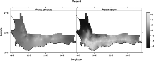
Figure 6: Posterior mean spatial effects ($\theta$) for Protea punctata (PRPUNC) and Protea repens (PRREPE). These effects offer local adjustment to potential abundance. Cells with values greater than zero represent regions with larger than expected populations, conditional on the other covariates.

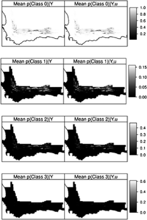
Figure 7: Abundance category probability maps for Protea punctata (PRPUNC) for untransformed (left) and transformed (right) situations. Values are cellwise posterior mean probabilities for the abundance classes. Class $0$ means the probability the species is absent, while classes $1$–$3$ indicate estimated abundance from $1$–$10$, $11$–$100$, $100{+}$ individuals, respectively.

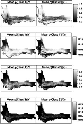
Figure 8: Abundance category probability maps for Protea repens (PRREPE) for untransformed (left) and transformed (right) situations. Values are cellwise posterior mean probabilities for the abundance classes. Class $0$ means the probability the species is absent, while classes $1$–$3$ indicate estimated abundance from $1$–$10$, $11$–$100$, $1008$ individuals, respectively.

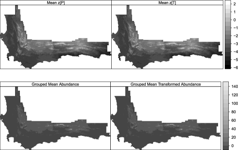
Figure 9: Mean posterior abundance summaries for Protea punctata (PRPUNC). On the latent $z$-scale, “Mean $z[P]$” refers to the potential abundance, while “Mean $z[T]$” refers to the potential abundance corrected for habitat transformation. The Grouped Mean Abundance rescales the Mean $z[P]$ surface to the expected potential size of a population in a grid cell (using the observed abundance classes: absent, $1$–$10$, $10$–$100$, $100{+}$). The Group Mean Transformed Abundance shows the expected size of a population after correcting for habitat transformation.

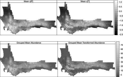
Figure 10: Mean posterior abundance summaries for Protea repens (PRREPE). On the latent $z$-scale, “Mean $z[P]$” refers to the potential abundance, while “Mean $z[T]$” refers to the potential abundance corrected for habitat transformation. The Grouped Mean Abundance rescales the Mean $z[P]$ surface to the expected potential size of a population in a grid cell (using the observed abundance classes: absent, $1$–$10$, $10$–$100$, $100{+}$). The Group Mean Transformed Abundance shows the expected size of a population after correcting for habitat transformation.

The mean posterior spatial effects are shown in Figure 6. Note that the spatial effects for the two species have quite different patterns, with Protea repens having a region of low values in the northeast and larger values elsewhere, while Protea punctata is more even across the landscape, but with lower values toward the edges of the CFR. These surfaces capture the spatial variability in abundance that is not explained by the other covariates within the model. This suggests that the covariates predict higher abundance of P. repens in the northwest than what was observed, perhaps indicating some unobserved limiting factor (such as unsuitable soils, more extreme seasonality in rainfall, or dispersal limitations). Similarly for P. punctata, the covariates may over-predict abundances at the edges of the CFR where many environmental factors change as one transitions to other biome types.

Figures 7 and 8 show the mean posterior abundance category probabilities (potential and transformed) for P. punctata (Figure 7) and P. repens (Figure 8). Comparing these plots among rows contrasts the probabilities associated with each abundance class for the species, while comparing between columns shows the effects of landscape transformations on abundance class probabilities. Both species show higher predicted abundances coinciding with mountainous areas of the CFR. This is where the fynbos biome dominates the landscape and where proteas are characteristically the dominant, indicator species [Rebelo et al. (2006)]. Note that P. punctata, a less common species, is only slightly affected by landscape transformation, while there are dramatic differences for P. repens (Figures 9 and 10). This is because P. punctata is mostly limited to dry, rocky, or shale slopes [Rebelo (2001)] which are less suitable for agriculture or development and thus mostly untransformed. P. repens, on the other hand, is much more ubiquitous across the region and can frequently occur in lowland areas that have been largely transformed by human activities [Rebelo (2001), Rebelo et al. (2006)].

It is also useful to summarize these data through mean potential abundance and mean transformed abundance (see Section 4.3) as in Figures 9 and 10. These figures allow inspection of the underlying latent surfaces that are of interest to ecologists as a continuous relative representation of species abundances. However, the latent “$z$” scales may be difficult to interpret ecologically and, thus, estimated potential and transformed abundance (using the grouped mean) are also shown. These represent the expected abundance (with respect to the $p$’s or $r$’s) of a species at a randomly selected sample location in that grid. The associated display makes it easy to visualize the effects of habitat transformation on protea populations. P. punctata shows almost no effects of landscape transformation, while large differences are apparent for P. repens. Note the large transformed regions in the south and west where the expected abundance of plants has dropped from more than 50 to near zero. It is also apparent that, across the landscape, P. punctata tends to have a higher expected mean abundance at any given sample point than does P. repens (Figures 9 and 10).

6 Discussion and future work

Building on previous efforts that have addressed the presence/absence of species, we have presented a modeling framework for learning about potential patterns for species abundance not degraded by land transformation and potential measurement error. The model was built using a hierarchical latent abundance specification, incorporating spatial structure to capture anticipated association between adjacent locations. Along with potential pattern, we also have an estimate of transformed abundance pattern. Comparison of these two patterns is helpful for understanding the effect of land transformation on species presence and abundance and, in particular, for disentangling these effects from those of other environmental factors. This may facilitate designing strategies for species conservation as well as understanding the overall effects of climate change.

This work has applications in biogeography and in conservation biology [Pearce and Ferrier (2001), Gaston (2003)]. We can now develop predictive maps of “high quality” habitat sites within a species range, based on high predicted abundances. This will help identify prime locations for effective conservation efforts. We can also estimate the impact of habitat transformation on the size of the population using the information from Figures 8 and 10, and thus identify threats to conservation. Predictive abundance maps will also be useful to explore patterns in biodiversity and species abundances. Do species abundances tend to peak in the middle of the species’ range [Gaston (2003)]? Do areas of high biodiversity tend to have lower species abundances? Are there areas that are rich in both abundance and biodiversity (perhaps identifying ideal regions for conservation efforts)?

There are several natural extensions. One is to study the temporal change in abundance. With abundance data collected over time as well as associated environmental factors such as rainfall and temperature, dynamic modeling of species abundance with changing environmental factors may give a clearer picture of how a species is responding to climate change. Indeed, when connected to future climate scenarios, we may attempt to forecast prospective species abundance. Similarly, if the transformation data is also time varying, we could illuminate the effect of land transformation in greater detail.

The current model uses transformation percentage $(1-u)$ in a deterministic way (transformation having a binary effect on potential abundance). In other cases (e.g., to study abundance pattern of animals) it may be reasonable to treat transformation as another covariate influencing species habitat. Also, it may be imagined that the relationship between potential abundance and environmental variables is not linear as specified in equation (3.3), for example, environmental variables may affect larger abundance classes differently from smaller abundance classes; piecewise linear specification, introducing different regression coefficients over the different abundance classes, could be explored.

Another possible extension lies in joint modeling of two or more species. One may wish to learn whether two plant varieties are sympatric or allopatric and whether or not there is evidence for competitive interactions or facilitation. Such modeling can be done by extending our model to have multiple $(z_{P,k},z_{T,k},z_{O,k})$ surfaces, where $k$ is the species indicator. Dependence can be introduced across $z_{P,k}$ surfaces by modeling $\theta^{(k)}$ using an MCAR [Gefand and Vounatsou (2003), Jin, Carlin and Banerjee (2005)]. Fitting such models will be very challenging if there are many grid cells.

Instead of taking an areal level approach, if covariate information is available at point level (where sampling sites are viewed as “points” within the large region, $D$), one may consider a point-level model. This amounts to replacing the CAR model with a Gaussian process prior for the spatial effects. With many sampling sites, we will need to use appropriate approximation techniques [Banerjee et al. (2008)].

Appendix

.1 Proof of $E(z_{T})$ finite

$E(z_{T})=E(E(z_{T}|z_{P}))=E(uz_{P}+(1-u)\times\break c(z_{P}))=E(z_{P}-(1-u)\frac{\phi(z_{P})}{1-\Phi(z_{P})})$. Assuming $z_{P}\sim N(\mu,1)$, it is enough to show $\int_{-\infty}^{\infty}\frac{\phi(x)}{1-\Phi(x)}\phi(x-\mu)\,dx<\infty$.

Consider the quantity $x^{2}\frac{\phi(x)}{1-\Phi(x)}\phi(x-\mu)$, if $x\rightarrow-\infty$, it goes to $0$. When $x\rightarrow\infty$, we have

$$\lim_{x\rightarrow\infty}x^{2}\frac{\phi(x)}{1-\Phi(x)}\phi(x-\mu)$$

$$\qquad\stackrel{{\scriptstyle L^{\prime}ptal}}{{=}}\lim_{x\rightarrow\infty}\frac{2x\phi(x)\phi(x-\mu)-x^{3}\phi(x)\phi(x-\mu)-x^{2}(x-\mu)\phi(x)\phi(x-\mu)}{-\phi(x)}$$

$$\hskip 4.0pt\qquad=0.$$

So $\lim_{|x|\rightarrow\infty}x^{2}\frac{\phi(x)}{1-\Phi(x)}\phi(x-\mu)=0$, thus, we can get $B_{1}<0,B_{2}>0$, such that $\frac{\phi(x)}{1-\Phi(x)}\phi(x-\mu)<\frac{1}{x^{2}}$ for all $x\notin(B_{1},B_{2})$. Hence, the result follows.

.2 Posterior simulation of $z$’s for a site with no presence observed

We subdivide by considering the ways that we can generate a $0$ realization of $y$ based on Equation (5) [one may also use Equation (3.3) to do this]:

1. [(iii)]

2. The area is untransformed, the species was potentially there, but missed during data collection or it was absent at that time instance; the event is $1_{z_{P}\geq\alpha_{0},z_{O}\leq\alpha_{0}}$ with prior probability $\pi_{1}=uP(z_{P}\geq\alpha_{0},z_{O}\leq\alpha_{0})$.

3. Potentially the species was absent there; the event is $1_{z_{P}\leq\alpha_{0}}$ with prior probability $\pi_{2}=P(z_{P}\leq\alpha_{0})$.

4. The species was potentially there $1_{z_{P}\geq\alpha_{0}}$, but the area was transformed; the event has prior probability $\pi_{3}=(1-u)P(z_{P}\geq\alpha_{0}).$

These three events are exhaustive and mutually exclusive for the event $(y=0)$. Thus, $f(z_{P},z_{O}|y=0,\Theta)$ is a $3$-component mixture. To draw a ($z_{P},z_{O}$) pair from this distribution amounts to first choosing a component and then drawing a pair ($z_{P},z_{O}$) from that component distribution. By Bayes’ rule, conditional on observed $(y=0)$, these three cases can happen with posterior probability $\pi_{i}/\sum_{l=1}^{3}\pi_{l},i=1,2,3$. So we use a multinomial to select which of these events took place. Before going into case by case details, it is worth mentioning that in all these cases the sampling from the joint density of chosen mixture component was done via the marginal $f(z_{P}|\cdot\cdot)$ followed by $f(z_{O}|z_{P},\cdot\ \cdot)$. The advantage of this scheme is that we don’t need to draw from the latter because $z_{O}$’s corresponding to $y=0$ are not involved in posterior full conditionals of any other parameters in the model (as $\alpha_{0}=0$, fixed). If the second case is selected, then $f(z_{O},z_{P}|\cdot,\cdot)\propto[u\delta_{z_{P}}+(1-u)\delta_{c(z_{P})}]1_{z_{O}\leq 0}1_{z_{P}\leq 0}\phi(z_{P})$ and thus marginalizing over $z_{O}$, we get $f(z_{P}|\cdot\cdot)\propto\phi(z_{P})1_{z_{P}\leq 0}$ which is a truncated Gaussian on $\mathbb{R^{-}}$. Similarly under case (iii), we need to simulate $z_{P}$ from $\phi(z_{P})1_{z_{P}\geq 0}$, a Gaussian truncated on $\mathbb{R^{+}}$. In case (i), $f(z_{O},z_{P}|\cdot\cdot)\propto\phi(z_{O};z_{P},1)1_{z_{P}\geq 0}1_{z_{O}\leq 0}\phi(z_{P})$, so marginalizing over $z_{O}$ we get $f(z_{P}|\cdot\cdot)\propto\phi(z_{P})(1-\Phi(z_{P}))1_{z_{P}\geq 0}$. An efficient way to draw from this density is to propose a $z_{P}$ from a truncated normal on $\mathbb{R^{+}}$ and do a Metropolis–Hastings update with an independent proposal, using the quantity $(1-\Phi(\cdot))$. However, all sampling distributions are summarized in Appendix .3 below.

.3 Posterior full conditionals needed for Gibbs sampling

• If $y_{ij}>0$, draw $z_{O,ij}\sim N(z_{P,ij},1)1_{(\alpha_{y_{ij}-1},\alpha_{y_{ij}})}$. Draw $z_{P,ij}\sim N(\frac{v_{i}^{T}\beta+\theta_{i}}{2}+\frac{z_{O,ij}}{2},\frac{1}{2})$.

• If $y_{ij}=0$, compute $p_{ij}=(u\Phi_{2}([0,\infty]\times[-\infty,0];\mu_{ij},\Sigma_{0}),1-\Phi(v_{i}^{T}\beta+\theta),(1-u)\Phi(v_{i}^{T}\beta+\theta_{i}))$, where $\mu_{ij}=(v_{i}^{T}\beta+\theta_{i},v_{i}^{T}\beta+\theta_{i})$ and $\Sigma_{0}=\left({{1\atop 1}\enskip{1\atop 2}}\right)$ are the location and dispersion parameters for bivariate normal joint prior distribution of $(z_{O,ij},z_{P,ij})$. Draw $d_{ij}\stackrel{{\scriptstyle\mathrm{i.i.d.}}}{{\sim}}\operatorname{mult}(p_{ij})$. If $d_{ij}=1$, propose $z_{P,ij}^{\mathit{propose}}\sim N(v_{i}^{T}\beta+\theta_{i},1)1_{(0,\infty)}$ and do a Metropolis–Hastings sampler using $(1-\Phi(\cdot))$. Else if $d_{ij}=2$, draw $z_{P,ij}\sim N(v_{i}^{T}\beta+\theta_{i},1)1_{(-\infty,0)}$, else draw $z_{P,ij}\sim N(v_{i}^{T}\beta+\theta_{i},1)1_{(0,\infty)}$.

• Draw $\alpha_{h}=\operatorname{unif}(\max_{ij:y_{ij}=h}z_{O,ij},\min_{ij:y_{ij}=h+1}z_{O,ij})$, $h=1,2$.

• Draw $\beta\sim$ $N(\mu_{\beta},\Sigma_{\beta})\prod_{i,j}N(z_{P,ij};v_{i},\beta,\theta_{i})$.

• Draw $\theta_{i}\sim$ $N(z_{P,ij};v_{i},\beta,\theta_{i})N(\frac{\sum_{j}w_{ij}\theta_{j}}{w_{i+}},\frac{\tau_{0}^{2}}{w_{i+}})$ for $i=1,2,\ldots,m$. Draw $\theta_{i}\sim$ $N(\frac{\sum_{j}w_{ij}\theta_{j}}{w_{i+}},\frac{\tau_{0}^{2}}{w_{i+}})$ for $i=m+1,2,\ldots,I$.

References

- Albert and Chib (1993) Albert, J. H. and Chib, S. (1993). Bayesian analysis of binary and polychotomous response data. J. Amer. Statist. Assoc. 88 670–679. \MR1224394
- Armstrong et al. (2003) Armstrong, M., Galli, A. G., Le Loc’h, G., Geffroy, F. and Eschard R. (2003). PluriGaussian Simulations in Geosciences. Springer, Berlin.
- Banerjee, Carlin and Gelfand (2004) Banerjee, S., Carlin, B. P. and Gelfand, A. E. (2004). Hierarchical Modeling and Analysis for Spatial Data. Chapman & Hall/CRC, Boca Raton, FL.
- Banerjee et al. (2008) Banerjee, S., Gelfand, A. E., Finley, A. O. and Sang, H. (2008). Gaussian predictive process models for large spatial datasets. J. Roy. Statist. Soc. Ser. B 70 825–848. \MR2523906
- Beale et al. (2007) Beale, C. M., Lennon, J. J., Elston, D. A., Brewer, M. J. and Yearsley, J. M. (2007). Red herrings remain in geographical ecology: A reply to Hawkins et al. Ecography 30 845–847.
- Besag (1974) Besag, J. (1974). Spatial interaction and the statistical analysis of lattice systems (with discussion). J. Roy. Statist. Soc. Ser. B 36 192–236. \MR0373208
- Besag and Kooperberg (1995) Besag, J. and Kooperberg, C. (1995). On conditional and intrinsic autoregressions. Biometrika 82 733–746. \MR1380811
- Busby (1991) Busby, J. R. (1991). BIOCLIM: A bioclimatic analysis and predictive system. In Nature Conservation: Cost Effective Biological Surveys and Data Analysis (C. R. Margules and M. P. Austin, eds.) 64–68. CSIRO, Canberra, Australia.
- Conroy et al. (2008) Conroy, M. J., Runge, J. P., Barker, R. J., Schofield, M. R. and Fonnesbeck, C. J. (2008). Efficient estimation of abundance for patchily distributed populations via two-phase, adaptive sampling. Ecology 89 3362–3370.
- Cressie et al. (2009) Cressie, N., Calder, C. A., Clark, J. S., Ver Hoef, J. M. and Wikle, C. K. (2009). Accounting for uncertainty in ecological analysis: The strengths and limitations of hierarchical statistical modeling. Ecological Applications 19 553–570.
- De Oliveira (2000) De Oliveira, V. (2000). Bayesian prediction of clipped Gaussian random fields. Comput. Statist. Data Anal. 34 299–314.
- Diggle, Menezes and Su (2010) Diggle, P. J., Menezes, R. and Su, T.-L. (2010). Geostatistical analysis under preferential sampling (with discussion). J. Roy. Statist. Soc. Ser. C 59 191–232.
- Elith et al. (2006) Elith, J., Graham, C. H., Anderson, R. P., Dudík, M., Ferrier, S., Guisan, A., Hijmans, R. J., Huettmann, F., Leathwick, J. R., Lehmann, A., Li, J., Lohmann, L. G., Loiselle, B. A., Manion, G., Moritz, C., Nakamura, M., Nakazawa, Y., Overton, J. McC., Peterson, A. T., Phillips, S. J., Richardson, K. S., Scachetti-Pereira, R., Schapire, R. E., Soberón, J., Williams, S., Wisz, M. S. and Zimmermann, N. E. (2006). Novel methods improve prediction of species’ distributions from occurrence data. Ecography 29 129–151.
- Fitzpatrick et al. (2008) Fitzpatrick, M. C., Gove, A. D., Nathan, J., Sanders, N. J. and Dunn, R. R. (2008). Climate change, plant migration, and range collapse in a global biodiversity hotspot: The Banksia (Proteaceae) of Western Australia. Global Change Biology 14 1337–1352.
- Fuller (1987) Fuller, W. A. (1987). Measurement Error Models. Wiley, New York. \MR0898653
- Gaston (2003) Gaston, K. (2003). The structure and dynamics of geographic ranges, 1st ed. Oxford Univ. Press, Oxford.
- Gelfand and Sahu (1999) Gelfand, A. E. and Sahu, S. K. (1999). Identifiability, improper priors, and Gibbs sampling for generalized linear models. J. Amer. Statist. Assoc. 94 247–253. \MR1689229
- Gefand and Vounatsou (2003) Gelfand, A. E. and Vounatsou, P. (2003). Proper multivariate conditional autoregressive models for spatial data analysis. Biostatistics 4 11–25.
- Gelfand et al. (2005a) Gelfand, A. E., Silander, J. A., Jr., Wu, S., Latimer, A. M., Lewis, P., Rebelo, A. G. and Holder, M. (2005a). Explaining species distribution patterns through hierarchical modeling. Bayesian Anal. 1 42–92. \MR2227362
- Gelfand et al. (2005b) Gelfand, A. E., Schmidt, A. M., Wu, S., Silander, J. A., Jr., Latimer, A. M. and Rebelo, A. G. (2005b). Modelling species diversity through species level hierarchical modeling. J. Roy. Statist. Soc. Ser. C 54 1–20. \MR2134594
- Goldblatt and Manning (2000) Goldblatt, P. and Manning, J. (2000). Cape Plants: A Conspectus of the Cape Flora of South Africa. National Botanical Institute of South Africa, Cape Town.
- Gorresen et al. (2009) Gorresen, P. M., McMillan, G. P., Camp, R. J. and Pratt, T. K. (2009). A spatial model of bird abundance as adjusted for detection probability. Ecography 32 291–298.
- Graham and Hijmans (2006) Graham, C. H. and Hijmans, R. J. (2006). A comparison of methods for mapping species ranges and species richness. Global Ecology and Biogeography 15 578–587.
- Guisan and Thuiller (2005) Guisan, A. and Thuiller, W. (2005). Predicting species distribution: Offering more than simple habitat models. Ecology Letters 8 993–1009.
- Guisan and Zimmerman (2000) Guisan, A. and Zimmerman, N. E. (2000). Predictive habitat distribution models in ecology. Ecological Modelling 135 147–186.
- Guisan et al. (2006) Guisan, A., Lehman, A., Ferrier, S., Austin, M. P., Overton, J. M. C., Aspinall, R. and Hastie, T. (2006). Making better biogeographical predictions of species’ distributions. Journal of Applied Ecology 43 386–392.
- Higgs and Hoeting (2010) Higgs, M. D. and Hoeting, J. A. (2010). A clipped latent-variable model for spatially correlated ordered categorical data. Comput. Statist. Data Anal. 54 1999–2011.
- Hooten, Larsen and Wikle (2003) Hooten, M. B., Larsen, D. R. and Wikle, C. K. (2003). Predicting the spatial distribution of ground flora on large domains using a hierarchical Bayesian model. Landscape Ecology 18 487–502.
- Ibáñez et al. (2009) Ibáñez, I., Silander, J. A., Jr., Allen, J. M., Treanor, S. and Wilson, A. (2009). Identifying hotspots for plant invasions and forecasting focal points of further spread. Journal of Applied Ecology 46 1219–1228.
- Jin, Carlin and Banerjee (2005) Jin, X., Carlin, B. P. and Banerjee, S. (2005). Generalized hierarchical multivariate CAR models for areal data. Biometrics 61 950–961. \MR2216188
- Kunin, Hartley and Lennon (2000) Kunin, W. E., Hartley, S. and Lennon, J. (2000). Scaling down: On the challenges of estimating abundance from occurrence patterns. The American Naturalist 156 560–566.
- Latimer et al. (2006) Latimer, A. M., Wu, S., Gelfand, A. E. and Silander, J. A., Jr. (2006). Building statistical models to analyze species distributions. Ecological Applications 16 33–50.
- Le Loc’h and Galli (1997) Le Loc’h, G. and Galli, A. (1997). Truncated plurigaussian method: Theoretical and practical points of view. In Geostatistics Wollongong’96 (E. Y. Baafi and N. A. Schofield, eds.) 1 211–222. Kluwer, Dordrecht, The Netherlands.
- Loarie et al. (2008) Loarie, S. R., Carter, B. E., Hayhoe, K., McMahon, S., Moe, R., Knight, C. A. and Ackerly, D. D. (2008). Climate change and the future of California’s endemic flora. PLoS ONE 3 e2502.
- Mallick and Gelfand (1995) Mallick, B. and Gelfand, A. E. (1995). Bayesian analysis of semiparametric proportional hazards models. Biometrics 51 843–852.
- Midgley and Thuiller (2007) Midgley, G. F. and Thuiller, W. (2007). Potential vulnerability of Namaqualand plant diversity to anthropogenic climate change. Journal of Arid Environments 70 615–628.
- Mueller-Dombois and Ellenberg (2003) Mueller-Dombois, D. and Ellenberg, H. (2003). Aims and Methods of Vegetation Ecology. Blackburn Press, Caldwell, NJ.
- Pearce and Ferrier (2001) Pearce, J. and Ferrier, S. (2001). The practical value of modelling relative abundance of species for regional conservation planning: A case study. Biological Conservation 98 33–43.
- Phillips and Dudík (2008) Phillips, S. J. and Dudík, M. (2008). Modeling of species distributions with Maxent: New extensions and a comprehensive evaluation. Ecography 31 161–175.
- Potts and Elith (2006) Potts, J. M. and Elith, J. (2006). Comparing species abundance models. Ecological Modelling 199 153–163.
- Pressey et al. (2007) Pressey, R. L., Cabeza, M., Watts, M. E., Cowling, R. M. and Wilson, K. A. (2007). Conservation planning in a changing world. Trends in Ecology and Evolution 22 583–592.
- Raxworthy et al. (2003) Raxworthy, C. J., Martinez-Meyer, E., Horning, N., Nussbaum, R. A., Schneider, G. E., Ortega-Huerta, M. A. and Peterson, A. T. (2003). Predicting distributions of known and unknown reptile species in madagascar. Nature 426 837–841.
- Rebelo (1991) Rebelo, A. G. (1991). Protea Atlas Manual: Instruction Booklet to the Protea Atlas Project. Protea Atlas Project, Cape Town.
- Rebelo (2001) Rebelo, A. G. (2001). Proteas: A Field Guide to the Proteas of Southern Africa, 2nd ed. Fernwood Press, Vlaeberg, South Africa.
- Rebelo (2002) Rebelo, A. G. (2002). The state of plants in the Cape Flora. In Proceedings of a Conference Held at the Rosebank Hotel in Johannesburg (G. H. Verdoorn and J. Le Roux, eds.) 18. The State of South Africa’s Species, Endangered Wildlife Trust.
- Rebelo (2006) Rebelo, A. G. (2006). Protea atlas project website. Available at http://protea.worldonline.co.za/default.htm.
- Rebelo et al. (2006) Rebelo, A. G., Boucher, C., Helme, N., Mucina, L. and Rutherford, M. C. (2006). Fynbos biome. In The Vegetation of South Africa, Lesotho and Swaziland. Streltzia (L. Micina and M. C. Rutherford, eds.) 19. South African National Biodiversity Institute, Pretoria, South Africa.
- Rouget et al. (2003) Rouget, M., Richardson, D. M., Cowling, R. M., Lloyd, J. W. and Lombard, A. T. (2003). Current patterns of habitat transformation and future threats to biodiversity in terrestrial ecosystems of the Cape Floristic Region, South Africa. Biological Conservation 112 63–83.
- Royle and Link (2006) Royle, J. A. and Link, W. A. (2006). Generalized site occupancy models allowing for false positive and false negative errors. Ecology 87 835–841.
- Royle et al. (2007) Royle, J. A., Kéry, M., Gautier, R. and Schmidt, H. (2007). Hierarchical spatial models of abundance and occurrence from imperfect survey data. Ecological Monographs 77 465–481.
- Schwartz et al. (2006) Schwartz, M. W., Iverson, L. R., Prasad, A. M., Matthews, S. N. and O’Connor, R. J. (2006). Predicting extinctions as a result of climate change. Ecology 87 1611–1615.
- Stefanski and Carroll (1987) Stefanski, L. A. and Carroll, R. J. (1987). Conditional scores and optimal scores for generalized linear measurement-error models. Biometrika 74 703–716. \MR0919838
- Sutherland (2006) Sutherland, W. J. (2006). Ecological Census Techniques, 2nd ed. Cambridge Univ. Press, Cambridge.
- Ver Hoef et al. (2001) Ver Hoef, J. M., Cressie, N., Fisher, R. N. and Case, T. J. (2001). Uncertainty and spatial linear models for ecological data. In Spatial Uncertainty in Ecology (C. T. Hunsaker, M. F. Goodchild, M. A. Friedl and T. J. Case, eds.) 214–237. Springer, New York.
- Ver Hoef and Frost (2003) Ver Hoef, J. M. and Frost, K. (2003). A Bayesian hierarchical model for monitoring harbor seal changes in Prince William Sound, Alaska. Environ. Ecol. Stat. 10 201–209. \MR1982484
- Wisz et al. (2008) Wisz, M. S., Hijmans, R. J., Li, J., Peterson, A. T., Graham, C. H. and Guisan, A. (2008). Effects of sample size on the performance of species distribution models. Diversity and Distributions 14 763–773.