Deuterated formaldehyde in $\rho$ Ophiuchi A

Abstract

Context. Formaldehyde is an organic molecule that is abundant in the interstellar medium. High deuterium fractionation is a common feature in low-mass star-forming regions. Observing several isotopologues of molecules is an excellent tool for understanding the formation paths of the molecules.

Aims. We seek an understanding of how the various deuterated isotopologues of formaldehyde are formed in the dense regions of low-mass star formation. More specifically, we adress the question of how the very high deuteration levels (several orders of magnitude above the cosmic D/H ratio) can occur using $\mathrm{H_{2}CO}$ data of the nearby $\rho$ Oph A molecular cloud.

Methods. From mapping observations of $\mathrm{H_{2}CO}$, $\mathrm{HDCO}$, and $\mathrm{D_{2}CO}$, we have determined how the degree of deuterium fractionation changes over the central $3^{\prime}\times 3^{\prime}$ region of $\rho$ Oph A. The multi-transition data of the various $\mathrm{H_{2}CO}$ isotopologues, as well as from other molecules (e.g., $\mathrm{CH_{3}OH}$ and $\mathrm{N_{2}D^{+}}$) present in the observed bands, were analysed using both the standard type rotation diagram analysis and, in selected cases, a more elaborate method of solving the radiative transfer for optically thick emission. In addition to molecular column densities, the analysis also estimates the kinetic temperature and $\mathrm{H_{2}}$ density.

Results. Toward the SM1 core in $\rho$ Oph A, the $\mathrm{H_{2}CO}$ deuterium fractionation is very high. In fact, the observed $\mathrm{D_{2}CO}$/$\mathrm{HDCO}$ ratio is $1.34\pm 0.19$, while the $\mathrm{HDCO}$/$\mathrm{H_{2}CO}$ ratio is $0.107\pm 0.015$. This is the first time, to our knowledge, that the $\mathrm{D_{2}CO}$/$\mathrm{HDCO}$ abundance ratio is observed to be greater than 1. The kinetic temperature is in the range 20-30 K in the cores of $\rho$ Oph A, and the $\mathrm{H_{2}}$ density is $(6-10)\times 10^{5}\,\mathrm{cm^{-3}}$. We estimate that the total $\mathrm{H_{2}}$ column density toward the deuterium peak is $(1-4)\times 10^{23}\,\mathrm{cm^{-2}}$. As depleted gas-phase chemistry is not adequate, we suggest that grain chemistry, possibly due to abstraction and exchange reactions along the reaction chain $\mathrm{H_{2}CO\to HDCO\to D_{2}CO}$, is at work to produce the very high deuterium levels observed.

1 Introduction

The study of deuterated molecules in the interstellar medium (ISM) has been intensified over the past decade ever since it was discovered that singly and multiply deuterated species (like the D-containing versions of $\mathrm{H_{2}CO}$, $\mathrm{CH_{3}OH}$, $\mathrm{NH_{3}}$) occurred at abundances that were orders of magnitude higher than would be expected from the local ISM D/H ratio of about $1.5\times 10^{-5}$ (Linsky 2003). The regions that show these elevated D-abundances are mainly associated with low-mass protostars. For instance, around IRAS16293$-$2422, Ceccarelli et al. (1998) and later Loinard et al. (2000) detected lines from doubly-deuterated formaldehyde ($\mathrm{D_{2}CO}$) which previously had only been seen in the Orion KL ridge (Turner 1990). Later, Loinard et al. (2002) extended the study to a larger set of protostars arriving at $\mathrm{D_{2}CO}$/$\mathrm{H_{2}CO}$ abundance ratios as high as 0.05-0.4. Likewise, high degrees of deuterium fractionation in $\mathrm{CH_{3}OH}$ (Parise et al. 2002, 2004, 2006) and $\mathrm{NH_{3}}$ (Roueff et al. 2000; Loinard et al. 2001; Lis et al. 2002) were subsequently discovered.

These studies are all related to single telescope pointings. To our knowledge, only one effort to delineate the $\mathrm{D_{2}CO}$/$\mathrm{H_{2}CO}$ abundance variation within a single source (IRAS16293$-$2422) has been made (Ceccarelli et al. 2001). The $\mathrm{D_{2}CO}$/$\mathrm{H_{2}CO}$ ratio peaks some $20^{\prime\prime}$ away from the protostar. Further out, the degree of deuteration seems to be lower in the quiscent gas (Ceccarelli et al. 2002). In the case of deuterated ammonia, the mapping study by Roueff et al. (2005) revealed that the deuterium peak is typically offset from the positions of the embedded protostars. These authors argued that the observed scenario could be explained by the formation of deuterium-enriched ices during the cold pre-collapse phase. At a later stage, a newly formed protostar evaporates the ices.

In their extensive study of deuterated $\mathrm{H_{2}CO}$ and $\mathrm{CH_{3}OH}$, Parise et al. (2006) concluded that formation of $\mathrm{CH_{3}OH}$ on grain surfaces was a likely explanation for the high degrees of deuterium fractionation seen in the various isotopologues. For $\mathrm{H_{2}CO}$, the situation was less clear and a formation path involving gas-phase reactions could not be ruled out. In fact, for the warmer Orion Bar PDR region, Parise et al. (2009) very recently advocated that gas-phase chemistry is entirely responsible for the deuterium fractionation seen for some singly deuterated species (including $\mathrm{HDCO}$). It should be noted that singly-deuterated species have been detected in dark and translucent clouds (Turner 2001) where the deuteration occurs only in the dense parts.

In interstellar clouds, deuterium is mostly molecular in the form of HD. Deuterium can be transferred from this main molecular reservoir to other molecules via exothermic reactions with the molecular ions $\mathrm{H_{3}^{+}}$, $\mathrm{CH_{3}^{+}}$, and $\mathrm{C_{2}H_{2}^{+}}$. These basic reactions are followed by efficient ion-neutral reactions and, in some cases, by reactions on grain surfaces. The exothermicity of the reactions involving these three molecular ions are in the range 230-550 K (Gerlich et al. 2002; Asvany et al. 2004; Herbst et al. 1987). As a result, deuterium fractionation is efficient in cold environments. It is also well established that a high degree of depletion on the grains of CO, O, and other heavy species, which would otherwise destroy efficiently H${}_{3}^{+}$ (and its deuterated analogues), is another important condition for deuterium fractionations taking place. Correlations between CO depletion and fractionation have been observed towards prestellar cores by, e.g., Bacmann et al. (2003) and Crapsi et al. (2005), and in the envelope of Class 0 protostars by Emprechtinger et al. (2009). Because of these two conditions (low temperature and high CO depletion), deuterium fractionation is particularly efficient during the early stages of star formation. The surface reactions on cold grains important for deuterium fractionation of $\mathrm{H_{2}CO}$ have recently been investigated through laboratory experiments (Hidaka et al. 2009).

The aforementioned low-mass protostar IRAS16293$-$2422 is located in the eastern part of the $\rho$ Ophiuchi cloud complex. To the west in the same complex, more than 1 degree away, lies the $\rho$ Oph A cloud (Loren et al. 1990) at a distance of about 120 pc (Lombardi et al. 2008; Loinard et al. 2008; Snow et al. 2008). This cloud core is well-studied by infrared, submillimeter, and millimeter continuum observations (Ward-Thompson et al. 1989; André et al. 1993; Motte et al. 1998). It hosts a well-collimated molecular outflow (André et al. 1990) and its driving source VLA 1623 (André et al. 1993). Moreover, it was in the direction of this cloud core that Larsson et al. (2007), using the Odin satellite, detected the 119 GHz line from molecular oxygen as well as the ammonia ground state line at 572 GHz (Liseau et al. 2003). More recently, while searching for the 234 GHz $\mathrm{O^{18}O}$ line Liseau et al. (2010) detected several lines due to $\mathrm{D_{2}CO}$ toward the millimeter continuum peaks. This study also includes $\mathrm{C^{18}O}$(3-2) mapping observations. Earlier, Loinard et al. (2002) reported a high $\mathrm{D_{2}CO}$/$\mathrm{H_{2}CO}$ ratio toward the VLA 1623 source. The existence of $\mathrm{D_{2}CO}$ in several positions of this $2^{\prime}\times 3^{\prime}$ cloud core formed the incentive of the present study as an excellent source to delineate the distribution of $\mathrm{H_{2}CO}$, $\mathrm{HDCO}$, and $\mathrm{D_{2}CO}$ as we know the distribution of the dust (Motte et al. 1998) and the gas in terms of $\mathrm{C^{18}O}$ (Liseau et al. 2010). Here we report on mapping observations of the $\rho$ Oph A cloud core in several frequency settings that cover most of the low-energy $\mathrm{H_{2}CO}$, $\mathrm{HDCO}$, and $\mathrm{D_{2}CO}$ lines in the 1.3 millimeter band using the 12 m APEX telescope (Güsten et al. 2006). In addition, lines from many other species were observed simultaneously (eg. $\mathrm{CH_{3}OH}$, $\mathrm{SO}$, and $\mathrm{N_{2}D^{+}}$). Here the $\mathrm{CH_{3}OH}$ results are of importance because $\mathrm{CH_{3}OH}$ is directly involved in the $\mathrm{H_{2}CO}$ chemistry and the $\mathrm{N_{2}D^{+}}$ results are, of course, of interest for the deuteration. Although the sulphur chemistry is not of immediate interest here we chose to include the $\mathrm{SO}$ and $\mathrm{SO_{2}}$ observational and analysis results since they are of importance as a complementary tool for determining the physical conditions. This paper is organized as follows. In Sect. (2) we describe the observations and then, in Sect. (3), we present the observational results. In Sect. (4) we obtain the physical conditions. Before concluding, in Sect. (6), we discuss our results in Sect. (5).

2 Observations

The APEX telescope at Chajnantor (Chile) was used to map the $3^{\prime}\times 3^{\prime}$ (with a spacing of $30\arcsec$) area centred on the coordinates $\alpha(\mathrm{J2000})={16}^{\mathrm{h}}\,{26}^{\mathrm{m}}\,{27.2}^{\mathrm{s}}$ and $\delta(\mathrm{J2000})={-24}\degr\,{23}\arcmin\,{34}\arcsec$ which is very close to the SM1N position in the $\rho$ Oph A cloud core as designated by André et al. (1993) in their submillimeter continuum maps. We used the single-sideband tuned APEX-1 receiver which is part of the Swedish heterodyne facility instrument (Vassilev et al. 2008). It has a sideband rejection ratio more than 10 dB. The image band is 12 GHz above or below the observing frequency depending on whether the tuning is optimized for operation in the upper or lower sidebands, respectively. For two frequency settings, the strong CO(2-1) and $\mathrm{C^{18}O}$(2-1) lines entered via the image band and from the strength we could estimate the sideband rejection ratio to be about 15 dB in both cases. As backend we used two 1 GHz modules of the FFTS (Klein et al. 2006). Each FFTS 1 GHz module has 8192 effective channels and the modules can be placed independently within the IF band width of 4-8 GHz. At 230 GHz this channel spacing corresponds to $0.16\,\mathrm{km\,s^{-1}}$ and the telescope beamsize (HPBW) is $27\arcsec$.

The telescope control software APECS (Muders et al. 2006) was used to control the raster mapping. All observations were performed in position-switching mode using a reference position offset by $300\arcsec$ east and $200\arcsec$ north of the map center. The pointing of the telescope was maintained and checked regularly by means of small CO(2-1) cross maps of the relatively nearby carbon stars IRAS15194$-$5115 and RAFGL1922. The determined pointing offsets were generally consistent from day to day and we believe we have an absolute pointing uncertainty better than $5\arcsec$. To optimize the antenna focussing we used continuum observations on Jupiter and Saturn.

The observations took place in two blocks and one additional day during 2009: April 24 - May 1, May 21, and July 4 - July 9. The column of precipitable water vapour was typically around 0.7 mm (varied between 0.3-2.9 mm). Typical system temperatures for the frequencies in question (218-252 GHz) were 200-220 K. The telescope main beam efficiency is $\eta_{\mathrm{mb}}=0.73$ at 345 GHz (Güsten et al. 2006). Hence, using the antenna surface accuracy of $18\,\mathrm{\mu m}$ we estimate that (using the Ruze formula) that the APEX main beam efficiency around 230 GHz is just slightly higher than at 345 GHz, about 0.75 which we adopt when converting the observed intensities from the $T_{\mathrm{A}}^{*}$ scale to the $T_{\mathrm{mb}}$ intensity scale. The heterodyne calibration procedure at APEX is more elaborate than the standard chopper wheel calibration scheme and involves three measurements by apart from the normal sky observation it also measures the receiver temperature by observing a hot and cold loads. Moreover, the atmospheric contribution is based on the model (Pardo et al. 2001) that has been adapted to the atmospheric characteristics at the Chajnantor site. The absolute calibration uncertainty is estimated to be 10% in the 1 mm band.

In Table 1 we summarize the targeted formaldehyde lines. The additional lines are summarized in Table 2. In the tables we include the line parameters: the transition frequency (typical uncertainty is 0.05 MHz or better), energy of lower level, and Einstein $A$-coefficient. These have been compiled from the Cologne Database of Molecular Spectroscopy (Müller et al. 2001, 2005). We here also indicate the symmetry due to the nuclear spin direction of the H (or D) nuclei, which for $\mathrm{H_{2}CO}$, $\mathrm{H_{2}^{13}CO}$ and $\mathrm{D_{2}CO}$ can be ortho (parallel spins) or para (anti-parallel spins). The statistical weight ratio of the symmetries is also noted if applicable. In the case of $\mathrm{CH_{3}OH}$, the internal rotation of the methyl group results in the symmetry species A and E. Note that radiative or non-reactive collisional transitions are forbidden between levels of different symmetry.

Table 1: Observed $\mathrm{H_{2}CO}$, $\mathrm{H_{2}^{13}CO}$, $\mathrm{HDCO}$, and $\mathrm{D_{2}CO}$ lines

Frequency	Transition	$E_{l}$	$A_{ul}$	Symmetry
(MHz)		(K)	($\mathrm{s}^{-1}$)
$\rm H_{2}CO$ ($o/p=3$)
218222.19	$3_{0,3}-2_{0,2}$	10.6	$2.8\times 10^{-4}$	para
218475.63	$3_{2,2}-2_{2,1}$	57.6	$1.6\times 10^{-4}$	para
218760.07	$3_{2,1}-2_{2,0}$	57.6	$1.6\times 10^{-4}$	para
225697.78	$3_{1,2}-2_{1,1}$	22.6	$2.8\times 10^{-4}$	ortho
$\rm H_{2}^{13}CO$ ($o/p=3$)
219908.52	$3_{1,2}-2_{1,1}$	22.4	$2.6\times 10^{-4}$	ortho
$\rm HDCO$
227668.45	$1_{1,1}-0_{0,0}$	0.0	$1.7\times 10^{-6}$
246924.60	$4_{1,4}-3_{1,3}$	25.8	$4.0\times 10^{-4}$
$\rm D_{2}CO$ ($o/p=2$)
221191.66	$4_{1,4}-3_{1,3}$	21.3	$2.9\times 10^{-4}$	para
231410.23	$4_{0,4}-3_{0,3}$	16.8	$2.8\times 10^{-4}$	ortho
233650.44	$4_{2,3}-3_{2,2}$	38.4	$2.7\times 10^{-4}$	ortho
234293.36a	$4_{3,2}-3_{3,1}$	65.4	$1.6\times 10^{-4}$	para
234331.06a	$4_{3,1}-3_{3,0}$	65.4	$1.6\times 10^{-4}$	para
245532.75	$4_{1,3}-3_{1,2}$	23.1	$3.9\times 10^{-4}$	para
a only observed at $(0,-30\arcsec)$

Table 2: Additional lines

Frequency	Transition	$E_{l}$	$A_{ul}$	Symmetry
(MHz)		(K)	($\mathrm{s}^{-1}$)
$\rm CH_{3}OH$ ($A/E=1$)
218440.05	$4_{2,2}-3_{1,2}$	35.0	$4.7\times 10^{-5}$	E
241700.22	$5_{0,5}-4_{0,4}$	36.3	$6.0\times 10^{-5}$	E
241767.22	$5_{1,5}-4_{1,4}$	28.8	$5.8\times 10^{-5}$	E
241791.43	$5_{0,5}-4_{0,4}$	23.2	$6.0\times 10^{-5}$	A
241879.07	$5_{1,4}-4_{1,3}$	44.3	$6.0\times 10^{-5}$	E
241904.15	$5_{2,4}-4_{2,3}$	49.1	$5.1\times 10^{-5}$	E
241904.65	$5_{2,3}-4_{2,2}$	45.5	$5.0\times 10^{-5}$	E
$\rm SO$
219949.44	$5_{6}-4_{5}$	24.4	$1.3\times 10^{-4}$
251825.77a	$6_{5}-5_{4}$	38.6	$2.0\times 10^{-4}$
$\rm{}^{34}SO$
246663.47	$6_{5}-5_{4}$	38.1	$1.8\times 10^{-4}$
$\rm SO_{2}$
226300.03	$14_{3,11}-14_{2,12}$	108.1	$1.1\times 10^{-4}$
241615.80	$5_{2,4}-4_{1,3}$	12.0	$8.5\times 10^{-5}$
245563.42	$10_{3,7}-10_{2,8}$	60.9	$1.2\times 10^{-4}$
$\rm{}^{34}SO_{2}$
219355.01	$11_{1,11}-10_{0,10}$	49.5	$1.1\times 10^{-4}$
241985.45	$8_{3,5}-8_{2,6}$	42.8	$1.1\times 10^{-4}$
246686.12	$4_{3,1}-4_{2,2}$	18.7	$8.4\times 10^{-5}$
$\rm N_{2}D^{+}$
231321.83	$3-2$	11.1	$7.1\times 10^{-4}$
a only observed at $(0,-30\arcsec)$

3 Results

In this section we will first display the formaldehyde mapping results of the $\rho$ Oph A cloud core, both as spectra, integrated intensity maps or velocity position diagrams where appropriate. After that, the mapping results for the other molecules will presented. Comparisons will be made with the existing APEX $\mathrm{C^{18}O}$(3-2) data at 329 GHz of Liseau et al. (2010) and the IRAM 30 m continuum map at 1.3 mm of Motte et al. (1998). The angular resolution of the two data sets is similar; the $\mathrm{C^{18}O}$ data have an HPBW of $19\arcsec$ while the 1.3 mm continuum map has an angular resolution of $15\arcsec$. Both these maps are shown in Fig. 1 where the 1.3 mm continuum map is shown in contours on top of a grey-scale image of the $\mathrm{C^{18}O}$(3-2) integrated intensity. The $3^{\prime}\times 3^{\prime}$ region shown in Fig. 1 corresponds to the area that has been mapped here in formaldehyde.

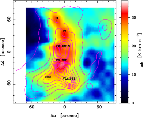
Figure 1: Colour image: The $\mathrm{C^{18}O}$(3-2) integrated intensity map of $\rho$ Oph A cloud core from Liseau et al. (2010). The intensity scale is shown to the right. Contours: The 1.3 mm continuum data by Motte et al. (1998). The contours start at 0.15 Jy with subsequent contours at every increment of 0.15 Jy. The flux densities are given in a $15\arcsec$ beam. We show the positions of the mm peaks from Motte et al. (1998) and the $\mathrm{C^{18}O}$ peaks of Liseau et al. (2010). The map offsets are given relative the position $\alpha(\mathrm{J2000})={16}^{\mathrm{h}}\,{26}^{\mathrm{m}}\,{27.2}^{\mathrm{s}}$ and $\delta(\mathrm{J2000})={-24}\degr\,{23}\arcmin\,{34}\arcsec$.

3.1 Formaldehyde results

All lines listed in Table 1 were detected except the ${1}_{1,1}-{0}_{0,0}$ transition of $\mathrm{HDCO}$ at 227 GHz. This transition has a much lower spontaneous rate coefficient than the other transitions. Two of the $\mathrm{D_{2}CO}$ lines were not mapped and were only observed in the $(0\arcsec,-30\arcsec)$ position. The typical rms in a map spectrum is in the range 0.06-0.1 K.

In Fig. 2 we plot the $\mathrm{H_{2}CO}$($3_{0,3}-2_{0,2}$) and $\mathrm{D_{2}CO}$($4_{0,4}-3_{0,3}$) spectra. They consist of 49 spectra separated by $30\arcsec$ on a 7x7 grid. The $\mathrm{H_{2}CO}$ lines posess a relatively complicated structure as compared to the $\mathrm{D_{2}CO}$ lines. The latter line shows only one velocity component around $3.8\,\mathrm{km\,s^{-1}}$ with full width at half maximum (FWHM) of $0.7\,\mathrm{km\,s^{-1}}$ and it is peaking strongly at the $(0\arcsec,-30\arcsec)$ position which, within the positional uncertainties, coincides with the SM1 or P3 position (cf. Fig. 1). We will hereafter refer to this position as the D-peak. The D-peak is also clearly seen in the integrated intensity maps of the three different $\mathrm{H_{2}CO}$ isotopologues (Fig. 3).

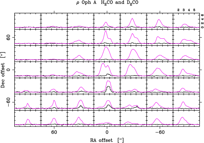
Figure 2: $\mathrm{H_{2}CO}$($3_{0,3}-2_{0,2}$) and $\mathrm{D_{2}CO}$($4_{0,4}-3_{0,3}$) map spectra toward the $\rho$ Oph A cloud. The $(0\arcsec,0\arcsec)$ position is the same as in Fig. 1. The vertical scale in each spectrum represents $T_{\mathrm{mb}}$ scale in K and the horizontal scale is velocity $v_{\mathrm{LSR}}$ with respect to local standard of rest in $\,\mathrm{km\,s^{-1}}$ as shown in the upper rightmost panel.

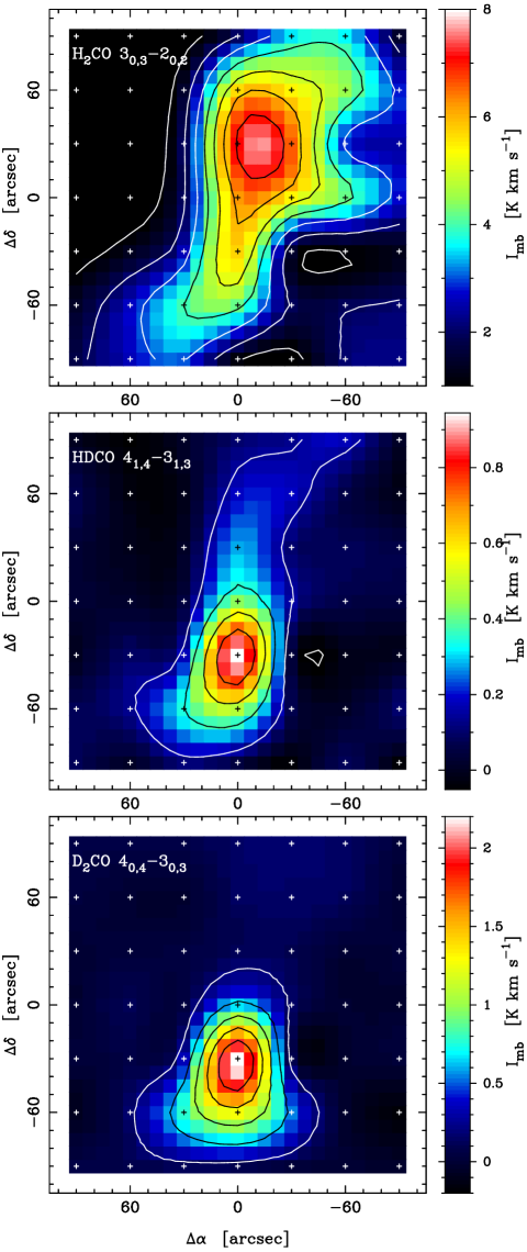
Figure 3: Maps of the $\mathrm{H_{2}CO}$($3_{0,3}-2_{0,2}$), $\mathrm{HDCO}$($4_{1,4}-3_{1,3}$), and $\mathrm{D_{2}CO}$($4_{0,4}-3_{0,3}$) integrated line intensity over the range $3.0-4.5\,\mathrm{km\,s^{-1}}$.

Maret et al. (2004) present a $\mathrm{H_{2}CO}$($3_{0,3}-2_{0,2}$) IRAM 30 m spectrum toward the position of VLA1623. The nearest position to VLA1623 in our map is at $(0\arcsec,-60\arcsec)$. The shape of our spectrum at this position is similar to the one presented by Maret et al. (2004) and our $T_{\mathrm{mb}}$ peak temperature of $3.8\,\mathrm{K}$ is slightly higher than theirs $T_{\mathrm{a}}^{\ast}/\eta_{\mathrm{mb}}\approx 2.2/0.62\approx 3.5\,\mathrm{K}$ despite the higher resolution of $11\arcsec$ in the IRAM 30 m spectrum. This would be expected for a relatively extended source which shows little variation on the scale of $11\arcsec-27\arcsec$. Also, from the distribution of the $\mathrm{H_{2}CO}$ emission we do not see any strong component that can be attributed to VLA1623.

The velocity as obtained from the $\mathrm{N_{2}H^{+}}$(1-0) observations by Di Francesco et al. (2004, 2009) (see also André et al. 2007) toward SM1 is $3.7\,\mathrm{km\,s^{-1}}$ with an FWHM of $0.6\,\mathrm{km\,s^{-1}}$, i.e. very similar to our values determined from the $\mathrm{D_{2}CO}$ lines at the D-peak. The peak intensity of the $\mathrm{D_{2}CO}$ line is about half that of $\mathrm{H_{2}CO}$. The size of $\mathrm{D_{2}CO}$ $4_{0,4}-3_{0,3}$ emission region (see Fig. 3), is found, by fitting a 2-dimensional gaussian, to be $33\arcsec\times 61\arcsec$. This size corresponds to a deconvolved source size of about $S=19\arcsec\times 55\arcsec$ for a beam size of $B=27\arcsec$. The filling factor when pointing the $27\arcsec$ beam toward the center of the source, is then $S^{2}/(S^{2}+B^{2})=(19\arcsec\times 55\arcsec)/(33\arcsec\times 61\arcsec)\approx 0.5$. This filling factor is merely an upper limit because any unresolved small-scale clumpiness may decrease the filling factor further.

In order to investigate the $\mathrm{H_{2}CO}$ line distribution over the $\rho$ Oph A cloud core we plot four velocity position diagrams (Fig. 4) between $\Delta\delta=\pm 90\arcsec$ at $\Delta\alpha=0\arcsec$. Here we also see that HDCO is peaking at the D-peak at $\Delta\delta=-30\arcsec$. Looking at the $\mathrm{HDCO}$ emission, there appears to be a velocity gradient over the D-peak source of about $0.2\,\mathrm{km\,s^{-1}}$ when going from $\Delta\delta=0\arcsec$ to $\Delta\delta=-60\arcsec$. It is also close to the D-peak where the $\mathrm{C^{18}O}$(3-2) emission has its maximum. The secondary $\mathrm{C^{18}O}$(3-2) peak (P1 in Fig. 1) is at $\Delta\delta=+30\arcsec$ and with a lower velocity of $\approx 3.1\,\mathrm{km\,s^{-1}}$ as compared to the velocity of $+3.7\,\mathrm{km\,s^{-1}}$ at the D-peak position and it is also here where the low-energy $\mathrm{H_{2}CO}$ line intensities reach their maximum value at $v_{\mathrm{LSR}}=3.3\,\mathrm{km\,s^{-1}}$. We denote this peak P1 from now on. There is also weak emission emanating from both $\mathrm{HDCO}$ and $\mathrm{D_{2}CO}$ at the $\Delta\delta=+30\arcsec$ position.

4

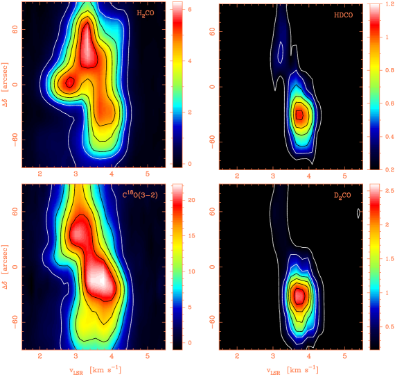
Figure 4: Velocity position diagrams of the $\mathrm{H_{2}CO}$($3_{0,3}-2_{0,2}$), $\mathrm{HDCO}$($4_{1,4}-3_{1,3}$), $\mathrm{D_{2}CO}$($4_{0,4}-3_{0,3}$), and $\mathrm{C^{18}O}$(3-2) lines along the declination axis at $\Delta\alpha=0^{\prime\prime}$. The molecule is indicated in each panel. The $\mathrm{C^{18}O}$(3-2) data are from Liseau et al. (2010). The vertical scale in each panel indicates the declination offset and the horizontal scale is the $v_{\mathrm{LSR}}$ velocity. The intensity scale in all four panels is $T_{\mathrm{mb}}$.

Interestingly, there is a third $\mathrm{H_{2}CO}$ peak at $\Delta\delta=0\arcsec$ and $v_{\mathrm{LSR}}\approx+2.9\,\mathrm{km\,s^{-1}}$ which has no obvious counterpart in the $\mathrm{C^{18}O}$ velocity position map. This peak makes the $\mathrm{H_{2}CO}$($3_{0,3}-2_{0,2}$) spectrum at $(0\arcsec,0\arcsec)$ to look doubly peaked (Fig. 2). However, these are two different cloud components and the dip is not an effect of self-absorption. This is evident from the velocity position diagrams in Fig. 4, but is also clear when comparing the $\mathrm{H_{2}^{13}CO}$($3_{1,2}-2_{1,1}$) and $\mathrm{H_{2}CO}$($3_{1,2}-2_{1,1}$) spectra. In Fig. 5 the central three spectra from the ortho lines $\mathrm{H_{2}CO}$($3_{1,2}-2_{1,1}$) and $\mathrm{H_{2}^{13}CO}$($3_{1,2}-2_{1,1}$) are displayed. Toward the $(0\arcsec,0\arcsec)$ position we see the doubly peaked line profile also for this $\mathrm{H_{2}CO}$ line, however there is no hint that the $\mathrm{H_{2}^{13}CO}$ line is peaking at the velocity of the dip for $\mathrm{H_{2}CO}$. If anything, the emission from the rarer species seems to follow that of the main species. We will return to the low-velocity component seen in the $(0\arcsec,0\arcsec)$ position below when we present the $\mathrm{CH_{3}OH}$ results.

5

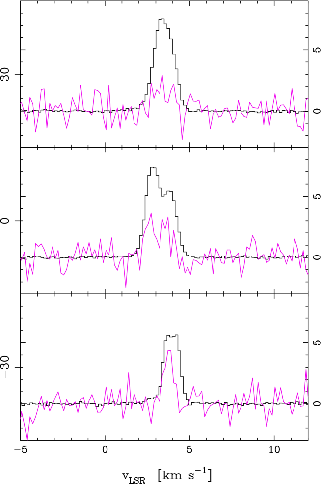
Figure 5: Ortho $\mathrm{H_{2}CO}$($3_{1,2}-2_{1,1}$) and $\mathrm{H_{2}^{13}CO}$($3_{1,2}-2_{1,1}$) spectra at declination offsets $-30\arcsec$ (bottom, D-peak), $0\arcsec$ (middle) and $+30\arcsec$ (top, P1). The offsets are relative the center position in Fig. 1. The $\mathrm{H_{2}^{13}CO}$ spectra (in colour) have been scaled up with a factor of 10 and appear much more noisy.

3.2 $\mathrm{CH_{3}OH}$ results

In Fig. 6 we show a map of the integrated intensity for the $\mathrm{CH_{3}OH}$ $5_{1,5}-4_{1,4}$ and $4_{2,2}-3_{1,2}$ E-lines. The latter line comes from levels of higher energy (Table 1). The distribution of $\mathrm{CH_{3}OH}$ is quite different from that of $\mathrm{H_{2}CO}$ (see Fig. 3). It should be noted that the $\mathrm{CH_{3}OH}$ $4_{2,2}-3_{1,2}$ line and the $\mathrm{H_{2}CO}$ lines at 218 GHz were observed simultaneously so the different distributions cannot be a result of large pointing offsets. The $\mathrm{CH_{3}OH}$ emission has its maximum at $(-30\arcsec,0)$ and in Fig. 7 all observed $5-4$ lines in this position are shown. Here the peak emission velocity is lower, around $v_{\mathrm{LSR}}\approx 2.8\,\mathrm{km\,s^{-1}}$. The cloud component at $(-30\arcsec,0\arcsec)$ extends into adjacent positions. The low-velocity feature seen for $\mathrm{H_{2}CO}$ (Fig. 4) is very likely associated with the $\mathrm{CH_{3}OH}$-peak. The higher energy $\mathrm{H_{2}CO}$ lines $3_{2,2/1}-2_{2,1/0}$ peak near this position. In addition, there is little $\mathrm{CH_{3}OH}$ at the D-peak position (Fig. 6).

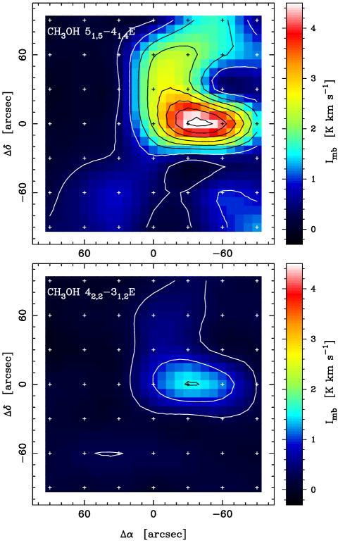
Figure 6: Integrated intensity maps of the $\mathrm{CH_{3}OH}$ $5_{1,5}-4_{1,4}$ and $4_{2,2}-3_{1,2}$ E-lines. First contour is at $0.3\,\mathrm{K\,km\,s^{-1}}$ and the increment is $0.6\,\mathrm{K\,km\,s^{-1}}$.

Figure 7: $\mathrm{CH_{3}OH}$ 5-4 lines around 241 GHz toward the $(-30\arcsec,0\arcsec)$ position. Note that the $5_{2,4}-4_{2,3}$ and $5_{2,3}-4_{2,2}$ E-lines are blended.

3.3 Results from other molecules

Two lines from $\mathrm{SO}$($5_{6}-4_{5}$) and $\mathrm{{}^{34}SO}$($6_{5}-5_{4}$) were covered during the observations. The map spectra are shown in Fig. 8. There is a single strong peak in the $\mathrm{{}^{34}SO}$ line intensity toward the position $(-60\arcsec,+60\arcsec)$ which we will call the S-peak. Here the $\mathrm{{}^{34}SO}$ and $\mathrm{SO_{2}}$ lines are very narrow, only about $0.4\,\mathrm{km\,s^{-1}}$. This is about twice the width one would expect from thermal broadening only (at $T_{\mathrm{kin}}=20\,\mathrm{K}$). Further west, at $(-90\arcsec,+30\arcsec)$, the $\mathrm{{}^{34}SO}$ line is broader, about $1.1\,\mathrm{km\,s^{-1}}$. The profile of $\mathrm{SO}$ shows line wings here which could be related to outflow activity. However, it is at the very border of our map and a clear delineation into red and blue wings are impossible. It should be pointed out that the S-peak has no structural counterpart in the $\mathrm{C^{18}O}$(3-2) map nor the 1.3 mm continuum map (cf. Fig. 1). Toward the D-peak, the $\mathrm{SO}$ lines exhibit a similar emission velocity ($v_{\mathrm{LSR}}\approx 3.7\,\mathrm{km\,s^{-1}}$) and line width ($\Delta v\approx 0.83\,\mathrm{km\,s^{-1}}$) as the other molecules. The covered $\mathrm{SO_{2}}$ and $\mathrm{{}^{34}SO_{2}}$ lines (Table 2) show a distribution similar to that of $\mathrm{SO}$ and $\mathrm{{}^{34}SO}$. At the P1-position the $\mathrm{SO}$ and $\mathrm{SO_{2}}$ emission velocity of about $\approx 2.9\,\mathrm{km\,s^{-1}}$ is lower than the velocity of $\approx 3.3\,\mathrm{km\,s^{-1}}$ for the formaldehyde isotopologues and $\mathrm{CH_{3}OH}$.

9

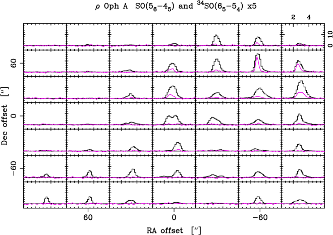
Figure 8: $\mathrm{SO}$($5_{6}-4_{5}$) and $\mathrm{{}^{34}SO}$($6_{5}-5_{4}$) map spectra toward the $\rho$ Oph A cloud. The $\mathrm{{}^{34}SO}$ spectra (in colour) have been multiplied with a factor of 5. Scales as in Fig. 2.

The deuterated version of $\mathrm{N_{2}H^{+}}$ (observed by Di Francesco et al. 2004, 2009; André et al. 2007), $\mathrm{N_{2}D^{+}}$(3-2) at 231 GHz was also covered during the formaldehyde observations. The integrated intensity map of $\mathrm{N_{2}D^{+}}$(3-2) is shown in Fig. 9. The peak intensity of the $\mathrm{N_{2}D^{+}}$ emission is clearly associated with the D-peak, with a secondary weaker source to the south-east. This secondary peak is not coincident with SM2 (see Fig. 1) but is located in the direction where the dust emission extends. Moreover, it shows up in the $\mathrm{N_{2}H^{+}}$ map of Di Francesco et al. (2004) and is designated N6 by them. The emission velocity of $\mathrm{N_{2}D^{+}}$(3-2) at the D-peak is $3.7\,\mathrm{km\,s^{-1}}$ and the FWHM is $0.85\,\mathrm{km\,s^{-1}}$ in agreement with what is found for the other species.

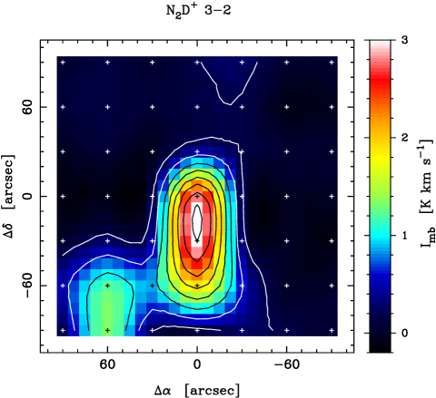
Figure 9: Integrated intensity map of the $\mathrm{N_{2}D^{+}}$ 3-2 line toward $\rho$ Oph A. First contour is at $0.2\,\mathrm{K\,km\,s^{-1}}$ and the increment is $0.4\,\mathrm{K\,km\,s^{-1}}$.

3.4 Result summary

After presenting the results of the distribution of the different molecules toward the $\rho$ Oph A cloud above we will now make a summary of the results which will be used in the analysis below. For $\mathrm{H_{2}CO}$ and $\mathrm{CH_{3}OH}$ we have identified three positions of interest which seem to represent distinctive sources; the D-peak at $(0\arcsec,-30\arcsec)$, the P1 peak at $(0\arcsec,+30\arcsec)$, and the $\mathrm{CH_{3}OH}$ peak at $(-30\arcsec,0\arcsec)$. In addition to these three peaks, the sulphur containing molecules are localized to $(-60\arcsec,+60\arcsec)$ (the S-peak). The emission velocities and FWHMs as obtained for the different species in these sources are summarized in Table 3 (from gaussian fits of the lowest energy lines in those cases where we have mapped multiple lines). Integrated line intensities for the relevant positions are tabulated in Table 4, Table 5, and Table 6. In these tables the $1\sigma$ uncertainties of the integrated intensities due to noise have been entered.

Table 3: Properties of the $\mathrm{H_{2}CO}$, $\mathrm{CH_{3}OH}$, $\mathrm{SO}$, and $\mathrm{SO_{2}}$ emission in selected cloud positions from gaussian fits

Offset	Molecule	$v_{\mathrm{LSR}}$	$\Delta v$ (FWHM)
		($\,\mathrm{km\,s^{-1}}$)	($\,\mathrm{km\,s^{-1}}$)
$(0\arcsec,-30\arcsec)$	$\mathrm{H_{2}CO}$	3.8(0.1)	0.95(0.05)
	$\mathrm{HDCO}$	3.6(0.1)	0.70(0.05)
	$\mathrm{D_{2}CO}$	3.8(0.1)	0.68(0.02)
	$\mathrm{CH_{3}OH}$	3.7(0.1)	0.73(0.05)
	$\mathrm{SO}$	3.7(0.1)	0.83(0.05)
	$\mathrm{SO_{2}}$	3.7(0.1)	0.67(0.05)
$(0\arcsec,+30\arcsec)$	$\mathrm{H_{2}CO}$	3.4(0.1)	1.20(0.05)
	$\mathrm{HDCO}$	3.2(0.1)	0.85(0.12)
	$\mathrm{D_{2}CO}$	3.2(0.1)	0.60(0.15)
	$\mathrm{CH_{3}OH}$	3.4(0.1)	1.18(0.05)
	$\mathrm{SO}$	3.0(0.1)	1.06(0.05)
	$\mathrm{SO_{2}}$	2.8(0.1)	0.77(0.05)
$(-30\arcsec,0\arcsec)^{a}$	$\mathrm{H_{2}CO}$	2.8(0.2)	0.95(0.10)
		3.6(0.2)	0.87(0.10)
	$\mathrm{CH_{3}OH}$	2.6(0.2)	0.62(0.10)
		3.2(0.2)	1.27(0.10)
$(-60\arcsec,+60\arcsec)$	$\mathrm{SO}$	3.0(0.1)	0.78 (0.05)
	$\mathrm{{}^{34}SO}$	2.9(0.1)	0.43(0.02)
	$\mathrm{SO_{2}}$	2.9(0.1)	0.42(0.02)
	$\mathrm{{}^{34}SO_{2}}$	3.0(0.1)	0.35(0.02)
a Fitted by two components, full intensity used in models

Table 4: $\mathrm{H_{2}CO}$, $\mathrm{H_{2}^{13}CO}$, $\mathrm{HDCO}$, and $\mathrm{D_{2}CO}$ integrated line intensities in three positions of the $\rho$ Oph A cloud

Molecule	Line	Frequency	$I_{\mathrm{mb}}=\int T_{\mathrm{mb}}\,dv$	$\Delta I_{\mathrm{mb}}$ a
		(MHz)	($\,\mathrm{K\,km\,s^{-1}}$)	($\,\mathrm{K\,km\,s^{-1}}$)
D-peak $(0\arcsec,-30\arcsec)$
$\mathrm{H_{2}CO}$	$3_{0,3}-2_{0,2}$	218222	6.07	0.05
	$3_{2,2}-2_{2,1}$	218476	0.83	0.05
	$3_{2,1}-2_{2,0}$	218760	0.80	0.05
	$3_{1,2}-2_{1,1}$	225698	6.88	0.06
$\mathrm{H_{2}^{13}CO}$	$3_{1,2}-2_{1,1}$	219908	0.26	0.06
$\mathrm{HDCO}$	$4_{1,4}-3_{1,3}$	246924	0.93	0.08
$\mathrm{D_{2}CO}$	$4_{1,4}-3_{1,3}$	221192	0.87	0.08
	$4_{0,4}-3_{0,3}$	231410	2.21	0.05
	$4_{2,3}-3_{2,2}$	233650	0.45	0.005
	$4_{3,2}-3_{3,1}$	234293	0.032	0.005
	$4_{3,1}-3_{3,0}$	234331	0.028	0.005
	$4_{1,3}-3_{1,2}$	245533	0.57	0.05
P1 $(0\arcsec,+30\arcsec)$
$\mathrm{H_{2}CO}$	$3_{0,3}-2_{0,2}$	218222	8.69	0.05
	$3_{2,2}-2_{2,1}$	218476	1.28	0.06
	$3_{2,1}-2_{2,0}$	218760	1.19	0.06
	$3_{1,2}-2_{1,1}$	225698	10.96	0.07
$\mathrm{H_{2}^{13}CO}$	$3_{1,2}-2_{1,1}$	219908	0.26	0.07
$\mathrm{HDCO}$	$1_{1,1}-0_{0,0}$	227668		0.06
	$4_{1,4}-3_{1,3}$	246924	0.44	0.05
$\mathrm{D_{2}CO}$	$4_{1,4}-3_{1,3}$	221192	0.13	0.05
	$4_{0,4}-3_{0,3}$	231410	0.19	0.05
$\mathrm{CH_{3}OH}$-peak $(-30\arcsec,0\arcsec)$
$\mathrm{H_{2}CO}$	$3_{0,3}-2_{0,2}$	218222	8.56	0.05
	$3_{2,2}-2_{2,1}$	218476	1.45	0.06
	$3_{2,1}-2_{2,0}$	218760	1.41	0.06
	$3_{1,2}-2_{1,1}$	225698	10.13	0.07
$\mathrm{H_{2}^{13}CO}$	$3_{1,2}-2_{1,1}$	219908	0.27	0.06
$\mathrm{HDCO}$	$4_{1,4}-3_{1,3}$	246924	0.12	0.05
$\mathrm{D_{2}CO}$	$4_{1,4}-3_{1,3}$	221192	0.12	0.05
	$4_{0,4}-3_{0,3}$	231410	0.15	0.05
a 1$\sigma$ error due to noise only

Table 5: $\mathrm{CH_{3}OH}$ integrated line intensities in three positions of the $\rho$ Oph A cloud

Line	Frequency	$I_{\mathrm{mb}}=\int T_{\mathrm{mb}}\,dv$	$\Delta I_{\mathrm{mb}}$ a
	(MHz)	($\,\mathrm{K\,km\,s^{-1}}$)	($\,\mathrm{K\,km\,s^{-1}}$)
D-peak $(0\arcsec,-30\arcsec)$
$4_{2,2}-3_{1,2}$E1	218440	0.21	0.05
$5_{0,5}-4_{0,4}$E1	241700	0.13	0.05
$5_{1,5}-4_{1,4}$E2	241767	0.72	0.05
$5_{0,5}-4_{0,4}$A	241791	0.81	0.05
$5_{1,4}-4_{1,3}$E1	241879	0.09	0.05
$5_{2,3/4}-4_{2,2/3}$E1	241904	0.07	0.05
P1 $(0\arcsec,+30\arcsec)$
$4_{2,2}-3_{1,2}$E1	218440	0.61	0.05
$5_{0,5}-4_{0,4}$E1	241700	0.59	0.05
$5_{1,5}-4_{1,4}$E2	241767	2.39	0.05
$5_{0,5}-4_{0,4}$A	241791	2.88	0.05
$5_{1,4}-4_{1,3}$E1	241879	0.20	0.05
$5_{2,3/4}-4_{2,2/3}$E1	241904	0.31	0.05
$\mathrm{CH_{3}OH}$-peak $(-30\arcsec,0\arcsec)$
$4_{2,2}-3_{1,2}$E1	218440	1.43	0.05
$5_{0,5}-4_{0,4}$E1	241700	1.49	0.05
$5_{1,5}-4_{1,4}$E2	241767	4.53	0.05
$5_{0,5}-4_{0,4}$A	241791	5.25	0.05
$5_{1,4}-4_{1,3}$E1	241879	0.96	0.05
$5_{2,3/4}-4_{2,2/3}$E1	241904	1.43	0.05
a 1$\sigma$ error due to noise only

Table 6: Integrated line intensities for other molecules in four positions of the $\rho$ Oph A cloud

Transition	Frequency	$I_{\mathrm{mb}}=\int T_{\mathrm{mb}}\,dv$	$\Delta I_{\mathrm{mb}}$ a
	(MHz)	($\,\mathrm{K\,km\,s^{-1}}$)	($\,\mathrm{K\,km\,s^{-1}}$)
D-peak $(0\arcsec,-30\arcsec)$
$\mathrm{SO}$($5_{6}-4_{5}$)	219949	7.22	0.06
$\mathrm{SO}$($6_{5}-5_{4}$)	251826	3.37	0.04
$\mathrm{{}^{34}SO}$($6_{5}-5_{4}$)	246663	0.19	0.03
$\mathrm{SO_{2}}$($5_{2,4}-4_{1,3}$)	241616	0.69	0.02
$\mathrm{SO_{2}}$($10_{3,7}-10_{2,8}$)	245563	0.16	0.04
$\mathrm{N_{2}D^{+}}$($3-2$)	231322	3.38	0.06
P1 $(0\arcsec,+30\arcsec)$
$\mathrm{SO}$($5_{6}-4_{5}$)	219949	13.1	0.06
$\mathrm{{}^{34}SO}$($6_{5}-5_{4}$)	246663	0.55	0.04
$\mathrm{SO_{2}}$($5_{2,4}-4_{1,3}$)	241616	1.70	0.05
$\mathrm{SO_{2}}$($10_{3,7}-10_{2,8}$)	245563	0.57	0.04
$\mathrm{N_{2}D^{+}}$($3-2$)	231322	0.37	0.08
$\mathrm{CH_{3}OH}$-peak $(-30\arcsec,0\arcsec)$
$\mathrm{SO}$($5_{6}-4_{5}$)	219949	8.25	0.06
$\mathrm{{}^{34}SO}$($6_{5}-5_{4}$)	246663	0.08	0.04
$\mathrm{SO_{2}}$($5_{2,4}-4_{1,3}$)	241616	0.23	0.05
$\mathrm{SO_{2}}$($10_{3,7}-10_{2,8}$)	245563	0.05	0.04
$\mathrm{N_{2}D^{+}}$($3-2$)	231322	0.17	0.07
S-peak $(-60\arcsec,+60\arcsec)$
$\mathrm{SO}$($5_{6}-4_{5}$)	219949	14.5	0.06
$\mathrm{{}^{34}SO}$($6_{5}-5_{4}$)	246663	1.31	0.04
$\mathrm{SO_{2}}$($5_{2,4}-4_{1,3}$)	241616	3.76	0.05
$\mathrm{SO_{2}}$($10_{3,7}-10_{2,8}$)	245563	1.14	0.04
$\mathrm{SO_{2}}$($14_{3,11}-14_{2,12}$)	226300	0.27	0.03
$\mathrm{{}^{34}SO_{2}}$($4_{3,1}-4_{2,2}$)	246686	0.24	0.04
$\mathrm{{}^{34}SO_{2}}$($8_{3,5}-8_{2,6}$)	241985	0.18	0.04
$\mathrm{{}^{34}SO_{2}}$($11_{1,11}-10_{0,10}$)	219355	0.46	0.04
$\mathrm{N_{2}D^{+}}$($3-2$)	231322		0.07
a 1$\sigma$ error due to noise only

4 Analysis

For several of the detected species (Table 4) we have multiple transitions that have significantly different energy levels. In such cases the so-called rotation diagram analysis (eg. Goldsmith & Langer 1999) can be employed to determine the rotation temperature, ${T_{\mathrm{rot}}}$, and the molecular column density, $N_{\mathrm{mol}}$. If all lines are optically thin, the rotation diagram method often is adequate to analyse multi-transition data. However, here it is likely that we have a mixture of optically thin and thick lines and therefore we adopt the modified approach to the rotation diagram method described by Nummelin et al. (2000). The modification involves the inclusion of the peak optical depth and thus, in addition to $T_{\mathrm{rot}}$ and $N_{\mathrm{mol}}$, also the beam filling factor, $\eta_{\mathrm{bf}}$, can be determined by minimization of a $\chi^{2}$-value. For a gaussian source distribution, $\eta_{\mathrm{bf}}$ is given by $\eta_{\mathrm{bf}}=S^{2}/(S^{2}+B^{2})$, where $S$ is the FWHM source size and $B$ is the FWHM beam size. If all transitions included in the analysis are optically thin and $\eta_{\mathrm{bf}}$ is set to 1 ($B<<S$), the method is very similar to the rotation diagram analysis with $N_{\mathrm{mol}}$ then representing a beam averaged column density.

In selected cases we will also check the results and refine the models obtained with the modified rotation diagram analysis by employing a more accurate treatment of the line excitation and radiative transfer. We have here adopted the accelerated lambda iteration (ALI) technique outlined by Rybicki & Hummer (1991, 1992). The ALI model cloud consists of spherically concentric shells and allows only for radial gradients of the physical parameters (kinetic temperature, molecular hydrogen density, molecular abundance, and radial velocity field). Moreover, and in contrast to the rotation diagram method, collisional excitation is included in the analysis, so the collision partner (here $\mathrm{H_{2}}$) density is a physical input parameter. The code used in the present work has been tested by Maercker et al. (2008) and it allows the inclusion of dust as a source of continuum emission in the shells. When the radiative transfer has been iteratively solved using the ALI approach, a model spectrum is produced by convolving the velocity dependent intensity distribution of the model cloud with a gaussian beam.

4.1 Analysis of the formaldehyde lines

As can be seen in Table 4 all four $\mathrm{H_{2}CO}$ lines are clearly detected in the three sources (D-peak, P1, and $\mathrm{CH_{3}OH}$-peak). The three para lines at 218 GHz have all been observed simultaneously so their relative strengths are not affected by any pointing or calibration uncertainties. The only ortho transition, the $3_{1,2}-2_{1,1}$ line at 225 GHz, was observed in a separate frequency setting. In our rotation diagram analysis we treat the ortho and para $\mathrm{H_{2}CO}$ lines together by assuming that the population distribution is determined by $T_{\mathrm{rot}}$ also between the states of different symmetry (through some exchange reaction or formation mechanism). For $\mathrm{H_{2}CO}$ the lowest ortho level ($1_{1,1}$) is about 15 K above the lowest para level ($0_{0,0}$). For $\mathrm{D_{2}CO}$ the reverse situation is in effect and it is the lowest level $0_{0,0}$ that is an ortho state while the lowest para level $1_{1,1}$ is 8 K higher up in energy. For a very low $T_{\mathrm{rot}}$ (during molecule formation) most of the molecules will be in the lowest energy state (para for $\mathrm{H_{2}CO}$ and ortho for $\mathrm{D_{2}CO}$). On the other hand, if $T_{\mathrm{rot}}$ is much greater than the energy difference of the symmetry states, the ortho to para population ratio will be governed by the statistical weight ratio which is $o/p=3$ for $\mathrm{H_{2}CO}$ and $o/p=2$ for $\mathrm{D_{2}CO}$.

In Table 7 the results of the modified rotation diagram analysis are shown. Here the number of lines used in the analysis for each molecule is tabulated together with best fit values of $T_{\mathrm{rot}}$, $N_{\mathrm{mol}}$, and $\eta_{\mathrm{bf}}$. In the last column, we list the minimum and maximum optical depths of the used transitions in the analysis. If there are not enough of lines or all lines are optically thin, one or two of the parameters have been set to a result obtained by another molecule in a previous fit. For instance, in the D-peak source, all three parameters could be determined in the analysis of $\mathrm{H_{2}CO}$, while for the optically thin $\mathrm{D_{2}CO}$ lines, $\eta_{\mathrm{bf}}$ had to be set to the value found for $\mathrm{H_{2}CO}$. Using the same $\eta_{\mathrm{bf}}$ for all formaldehyde isotopologues will also make the determined column densities directly comparable with each other. Interestingly, the $T_{\mathrm{rot}}$ obtained for $\mathrm{D_{2}CO}$, $17.4\,\mathrm{K}$ toward the D-peak is lower than that found for $\mathrm{H_{2}CO}$ ($T_{\mathrm{rot}}=22.5\,\mathrm{K}$). We assume this is an effect of subthermal excitation and difference in optical depths, where the higher optical depths for $\mathrm{H_{2}CO}$ make the excitation more efficient via photon trapping as compared to $\mathrm{D_{2}CO}$. A lower rotation temperature of the less abundant formaldehyde isotopologues was also seen in IRAS16293$-$2422 by Loinard et al. (2000) and in several other sources by Parise et al. (2006). For the other two sources (the P1 and $\mathrm{CH_{3}OH}$ peaks) the number of detected $\mathrm{D_{2}CO}$ transitions is not sufficient to allow for a $T_{\mathrm{rot}}$ determination and we assume that the ratio of $T_{\mathrm{rot}}$($\mathrm{D_{2}CO}$)/$T_{\mathrm{rot}}$($\mathrm{H_{2}CO}$) is the same in these two sources as in the D-peak source. The deduced $T_{\mathrm{rot}}$ is higher in the P1 and $\mathrm{CH_{3}OH}$ peaks than in the D-peak. This could be expected because the ratio of the $3_{0,3}-2_{2,0}$ and $3_{2,2}-2_{2,1}$ $\mathrm{H_{2}CO}$ lines is a good measure of kinetic temperature (Mangum & Wootten 1993) and this ratio is highest toward the $\mathrm{CH_{3}OH}$-peak. Of course, from the models we can also estimate the intensity of lines not included in the analysis. In particular, we find for the $\mathrm{HDCO}$ $1_{1,1}-0_{0,0}$ line that for the determined model parameters toward the D-peak its expected intensity is about 5 times below the noise level, consistent with our non-detection.

Table 7: Analysis results for $\mathrm{H_{2}CO}$, $\mathrm{H_{2}^{13}CO}$, $\mathrm{HDCO}$, $\mathrm{D_{2}CO}$, $\mathrm{CH_{3}OH}$, $\mathrm{SO}$, and $\mathrm{SO_{2}}$ from using the modified rotation diagram technique

Molecule	No. of	$T_{\mathrm{rot}}$	$N_{\mathrm{mol}}$	$\eta_{\mathrm{bf}}$	$\tau_{\mathrm{min}},\tau_{\mathrm{max}}$
	lines	(K)	$\mathrm{cm^{-2}}$
D-peak $(0\arcsec,-30\arcsec)$
$\mathrm{H_{2}CO}$	4	22.5	$2.22\times 10^{14}$	0.446	0.11,2.70
$\mathrm{D_{2}CO}$	6	17.4	$3.17\times 10^{13}$	(0.446)	0.01,0.54
$\mathrm{HDCO}$	1	(17.4)	$2.37\times 10^{13}$	(0.446)	0.23
$\mathrm{H_{2}^{13}CO}$	1	(17.4)	$4.09\times 10^{12}$	(0.446)	0.06
$\mathrm{CH_{3}OH}$	6	6.8	$7.21\times 10^{14}$	1	0.02,0.62
$\mathrm{SO}$	2	18.3	$2.38\times 10^{14}$	(1)	0.50,1.21
$\mathrm{{}^{34}SO}$	1	(18.3)	$9.67\times 10^{12}$	(1)	0.02
$\mathrm{SO_{2}}$	2	19.9	$4.23\times 10^{13}$	(1)	0.01,0.07
P1 $(0\arcsec,+30\arcsec)$
$\mathrm{H_{2}CO}$	4	25.9	$1.90\times 10^{14}$	0.469	0.10,1.91
$\mathrm{D_{2}CO}$	2	(20)	$1.66\times 10^{12}$	(0.469)	0.01,0.02
$\mathrm{HDCO}$	1	(20)	$6.21\times 10^{12}$	(0.469)	0.05
$\mathrm{H_{2}^{13}CO}$	1	(20)	$1.71\times 10^{12}$	(0.469)	0.02
$\mathrm{CH_{3}OH}$	6	7.4	$1.24\times 10^{15}$	1	0.05,1.20
$\mathrm{SO_{2}}$	2	23.4	$9.91\times 10^{13}$	(1)	0.04,0.12
$\mathrm{CH_{3}OH}$-peak $(-30\arcsec,0\arcsec)$
$\mathrm{H_{2}CO}$	4	26.3	$2.66\times 10^{14}$	0.325	0.14,2.60
$\mathrm{D_{2}CO}$	2	(20)	$1.93\times 10^{12}$	(0.325)	0.01,0.03
$\mathrm{HDCO}$	1	(20)	$2.38\times 10^{12}$	(0.325)	0.02
$\mathrm{H_{2}^{13}CO}$	1	(20)	$3.58\times 10^{12}$	(0.325)	0.05
$\mathrm{CH_{3}OH}$	6	9.2	$1.26\times 10^{15}$	1	0.11,1.46
$\mathrm{SO_{2}}$	1	(20)	$8.33\times 10^{12}$	(1)	0.01
S-peak $(-60\arcsec,+60\arcsec)$
$\mathrm{SO_{2}}$	3	19.7	$7.63\times 10^{14}$	1	0.04,1.21
$\mathrm{{}^{34}SO_{2}}$	2	(19.7)	$5.63\times 10^{13}$	(1)	0.04,0.05
A value surrounded by (…) indicates a fixed parameter.

The derived $\mathrm{H_{2}CO}$ rotation temperatures for the three cores are quite similar to the ones obtained by Parise et al. (2006) for other low-mass protostar sources. Likewise, the derived $\mathrm{H_{2}CO}$ column densities are just slightly higher than the corresponding rotation diagram values of Parise et al. (2006). The filling factor $\eta_{\mathrm{bf}}=0.446$ determined toward the D-peak is in agreement with the filling of $\sim 0.5$ determined from the $\mathrm{D_{2}CO}$ $4_{0,4}-3_{0,3}$ source size in Sect. (3.1).

4.2 Analysis of the methanol lines

The $\mathrm{CH_{3}OH}$ analysis using the modified rotation diagram technique is based on the integrated line intensities listed in Table 5. In all sources 6 $\mathrm{CH_{3}OH}$ lines with lower state energies ranging from 23 to 46 K, have been used. In the D-peak source a couple of lines are just marginally detected but are included in the best fit analysis since they are weighted with the uncertainty and do not affect the fit significantly. The line feature at 241904 MHz is a blend of two $\mathrm{CH_{3}OH}$ lines of about the same energy and $A$-coefficient and we have not been able to clearly resolve them into individual components. All lines at 241 GHz were observed simultaneously. The only $\mathrm{CH_{3}OH}$ line not belonging to the 241 GHz $5-4$ line forest is the $4_{2,2}-3_{1,2}$ E-line which is located in the 218 GHz $\mathrm{H_{2}CO}$-band.

Only one line from the methanol A-species has been observed and included in the analysis. Just like in the case of ortho and para formaldehyde, the A- and E-species of methanol are treated together. The energy difference between the lowest A and E-methanol states is 8 K with the A-species having the lowest energy. Furthermore, we only consider methanol to be in its lowest torsional state.

The best fit results in the $\mathrm{CH_{3}OH}$ analysis have been entered in Table 7. In all three sources we find a low $T_{\mathrm{rot}}$ of 7 to 9 K. Also the $\eta_{\mathrm{bf}}$ is found to be very close to 1. The much lower rotation temperatures found in the $\mathrm{CH_{3}OH}$ analysis as compared to the $\mathrm{H_{2}CO}$ and $\mathrm{D_{2}CO}$ results suggest that the excitation of $\mathrm{CH_{3}OH}$ is quite sub-thermal and a more elaborate treatment of the excitation and radiative transfer is needed (as was demonstrated by Bachiller et al. (1998) in their Fig. 9a). This is also supported by the fact that none of the $\mathrm{CH_{3}OH}$ fits are good since several of the modelled line intensities deviate substantially from the observed line intensities.

4.3 ALI modelling

Our aim with the non-LTE modelling using the ALI code is to construct a homogeneous (in terms of physical parameters but not in terms of excitation which may vary radially) spherical model cloud, for each of the source positions (D-, P1, and $\mathrm{CH_{3}OH}$-peaks), that produces the observed $\mathrm{H_{2}CO}$ and $\mathrm{CH_{3}OH}$ spectra. The results from the modifed rotation diagram analysis above are used as a guide when adopting the model cloud parameters. The ALI setup for the statistical equilibrium equations includes collisional excitation rates and for formaldehyde we use the He-$\mathrm{H_{2}CO}$ collisional coefficients calculated by Green (1991). The coefficients have been multiplied by 2.2 to approximate the $\mathrm{H_{2}}$-$\mathrm{H_{2}CO}$ collision system. For the $\mathrm{H_{2}}$-$\mathrm{CH_{3}OH}$ collision coefficients we adopt those of Pottage et al. (2004). For both species only levels below 200 K are included and we divide the model cloud into 29 shells. We do not include any radial velocity field in the source and instead we simply use a microturbulent velocity width, $v_{\mathrm{turb}}$, that reproduces the observed line widths. For an optically thin line, the FWHM line width is $\sqrt{4\ln 2}\,v_{\mathrm{turb}}$.

The results of the three ALI models have been summarized in Table 8. The listed cloud radii $R$ (in the first column) are based on the corresponding $\mathrm{H_{2}CO}$ beam filling results (Table 7) and a distance to $\rho$ Oph A of 120 pc. The tabulated column densities are the source-averaged values $2\,N_{\mathrm{peak}}/3$, where $N_{\mathrm{peak}}$ is the column density through the center of the spherical model cloud. It should be noted that the derived $n(\mathrm{H_{2}})$ (and hence $N(\mathrm{H_{2}})$) is a compromise value since, for all three models, a 20% lower value yields better fits for $\mathrm{CH_{3}OH}$ while a similarly higher value is optimum for $\mathrm{H_{2}CO}$. However, as the differences are less than about 50% any real difference in ${n(\mathrm{H_{2}})}$ is within the uncertainties of the adopted collisional coefficients. The ortho-to-para ratio is about 2 for all three models but since the ortho results are based on a single optically thick line ($\tau\sim 4$) only and not observed simultaneously with the three para lines, we cannot really exclude ortho-to-para ratios in the range 1-3. The derived $\mathrm{H_{2}CO}$ column densities are about 30% lower than those derived from the modified rotation diagram analysis. In contrast to $N(\mathrm{H_{2}CO})$ and $N(\mathrm{H_{2}})$ which do not vary much among the three cores, the $\mathrm{CH_{3}OH}$ column densities vary from $5\times 10^{13}\,\mathrm{cm^{-2}}$ in the D-peak to $4\times 10^{14}\,\mathrm{cm^{-2}}$ at the $\mathrm{CH_{3}OH}$-peak position. In addition, the E/A $\mathrm{CH_{3}OH}$ ratios seem to be close to 1 and since the A-line is observed simultaneously with the E-lines the determined A/E-ratio of 1 is less uncertain than the estimated ortho/para ratios for formaldehyde. The optical depth for the strongest of the $\mathrm{CH_{3}OH}$ lines are about 0.5-0.6 toward the $\mathrm{CH_{3}OH}$-peak. The total $\mathrm{H_{2}}$ mass of a core is about $0.1-0.2\,\mathrm{M}_{\odot}$.

Table 8: Model cloud properties and results for the ALI analysis

Source	$R/10^{16}$	$v_{\mathrm{turb}}$	$T_{\mathrm{kin}}$	$n(\mathrm{H_{2}})$	$N(\mathrm{H_{2}})$	$M(\mathrm{H_{2}})$	$X[\mathrm{H_{2}CO}]$$\times 10^{9}$		$N(\mathrm{H_{2}CO})$	$X[\mathrm{CH_{3}OH}]$$\times 10^{9}$		$N(\mathrm{CH_{3}OH})$
	(cm)	($\mathrm{km\,s^{-1}}$)	(K)	($\mathrm{cm^{-3}}$)	($\mathrm{cm^{-2}}$)	($\mathrm{M}_{\odot}$)	para	ortho	($\mathrm{cm^{-2}}$)	A	E	($\mathrm{cm^{-2}}$)
D-peak	3.3	0.4	24	$6\times 10^{5}$	$3\times 10^{22}$	0.16	$1.8$	$3.6$	$1.5\times 10^{14}$	$0.9$	$0.9$	$5.0\times 10^{13}$
P1	3.4	0.6	27	$7\times 10^{5}$	$3\times 10^{22}$	0.18	$1.7$	$3.3$	$1.5\times 10^{14}$	$2.0$	$2.0$	$1.2\times 10^{14}$
$\mathrm{CH_{3}OH}$-peak	2.7	0.6	30	$1\times 10^{6}$	$4\times 10^{22}$	0.14	$1.7$	$3.3$	$1.8\times 10^{14}$	$5.3$	$5.8$	$4.0\times 10^{14}$

To our knowledge, there are no collision coefficients available for the collision system $\mathrm{H_{2}}$-$\mathrm{D_{2}CO}$, so we cannot use our ALI model for $\mathrm{D_{2}CO}$. However, using the $\mathrm{H_{2}}$-$\mathrm{H_{2}CO}$ collision rates we check what happens to the excitation temperatures when adopting a factor of 7 lower column density (the ratio of $N$($\mathrm{H_{2}CO}$) and $N$($\mathrm{D_{2}CO}$) in Table 7 is close to 7). We then find that the excitation temperatures of the $3_{1,2}-2_{1,1}$ transition drop between 20-30% at different radii. This drop in excitation temperature is in line with the 20% lower $T_{\mathrm{rot}}=17.4\,\mathrm{K}$ found for $\mathrm{D_{2}CO}$ as compared to $\mathrm{H_{2}CO}$ value of $T_{\mathrm{rot}}=22.5\,\mathrm{K}$ found toward the D-peak. Hence, it is quite plausible that the lower rotation temperature found for $\mathrm{D_{2}CO}$ as compared to $\mathrm{H_{2}CO}$ can be explained by less efficient photon trapping in the excitation of $\mathrm{D_{2}CO}$. We also checked the influence on our results by continuum emission of dust, and the inclusion of a dust component with standard dust parameters ($T_{\mathrm{d}}=22\,\mathrm{K}$, gas-to-dust mass ratio of 100) had negligible impact on our modelling results.

Liseau et al. (2003) report results from a large velocity gradient (LVG) analysis of the $\rho$ Oph A using $\mathrm{CH_{3}OH}$ $2-1$ and $3-2$ line forest data, at 96 and 145 GHz, obtained by SEST at an angular resolution larger ($52^{\prime\prime}$ and $35^{\prime\prime}$) than for the present study. The analysed data were averaged from spectra spaced by $30\arcsec$ in the north-south direction around the P2 position (see Fig. 1) and their spectra is thus a partial blend of the contribution of the three cores. This is especially the case for their $2-1$ observations. However, their LVG results ($T_{\mathrm{kin}}=20\,\mathrm{K}$, $n(\mathrm{H_{2}})=4.5\times 10^{5}\,\mathrm{cm^{-3}}$, $X[\mathrm{CH_{3}OH}]=2.7\times 10^{-9}$) are in good agreement with those reported here.

4.4 Analysis of other molecules

In the S-peak position we have detected three $\mathrm{SO_{2}}$ lines and a modified rotation diagram analysis gave best-fit results for $\eta_{\mathrm{bf}}$ very close to 1. For $\mathrm{SO_{2}}$ we find a rotation temperature of about 20 K and a column density of $N(\mathrm{SO_{2}})=7.6\times 10^{14}\,\mathrm{cm^{-2}}$. The same analysis was made for two of the three detected $\mathrm{{}^{34}SO_{2}}$ lines and we get $N(\mathrm{{}^{34}SO_{2}})=5.6\times 10^{13}\,\mathrm{cm^{-2}}$ when using the rotation temperature of the more common variant. The $11_{1,11}-10_{0,10}$ $\mathrm{{}^{34}SO_{2}}$ line was excluded in the fit since its observed strength is incompatible (too strong by about a factor of 2) with the rotation temperature found for $\mathrm{SO_{2}}$, cf. Table 6. The reason for this is unclear but could be due to an unknown blend or a non-LTE effect involving $K_{a}=0$ states. Likewise, the two SO lines detected toward the D-peak position result in a rotation temperature of 18 K and a column density of $2.4\times 10^{14}\,\mathrm{cm^{-2}}$ (again assuming $\eta_{\mathrm{bf}}=1$). In the P1 position, the two detected $\mathrm{SO_{2}}$ lines give $T_{\mathrm{rot}}=23\,\mathrm{K}$ and a beam averaged column density of $9.9\times 10^{13}\,\mathrm{cm^{-2}}$. Furthermore, assuming $T_{\mathrm{rot}}=20\,\mathrm{K}$ we arrive at a beam averaged $\mathrm{SO_{2}}$ column density of $8.3\times 10^{12}\,\mathrm{cm^{-2}}$ toward the $\mathrm{CH_{3}OH}$-peak. The $\mathrm{SO}$ and $\mathrm{SO_{2}}$ results have been entered in Table 7.

The analysis results of the other molecules are summarized in Table 9. The column densities listed here are all calculated under the assumption of optically thin emission. The $\mathrm{C^{18}O}$(3-2) column densities are based on the data from Liseau et al. (2010) and have been derived using the kinetic temperatures derived from the ALI analysis as excitation temperature as the lower $\mathrm{C^{18}O}$ transitions are expected to be thermalized at the high densities of the cores. For the S-peak, the $\mathrm{SO_{2}}$ rotation temperature of 20 K was used as excitation temperature for all molecules. Also tabulated is the $N$($\mathrm{H_{2}}$) column density deduced from $N$($\mathrm{C^{18}O}$) and assuming a $\mathrm{C^{18}O}$ abundance of $X[\mathrm{C^{18}O}]=2\times 10^{-7}$ (standard value of undepleted gas interstellar gas, Frerking et al. (1982), but see also Wouterloot et al. (2005) for a discussion applicable to the $\rho$ Oph cloud). In this context it is enlightning to estimate how much the cores contribute to the observed $\mathrm{C^{18}O}$(3-2) integrated line intensity. Adopting the physical parameters (Table 8) and assuming $X[\mathrm{C^{18}O}]=2\times 10^{-7}$ we find, using the ALI code for $\mathrm{C^{18}O}$, that the cores make up 31%, 37%, and 67% of the observed $\mathrm{C^{18}O}$(3-2) emission in the D-, P1-, and $\mathrm{CH_{3}OH}$-cores, respectively. Firstly, this tells us that the $\mathrm{C^{18}O}$ abundance in the cores cannot be much higher than $2\times 10^{-7}$ as they then would produce too much $\mathrm{C^{18}O}$(3-2) emission. Secondly, an appreciable part of the observed $\mathrm{C^{18}O}$(3-2) emission is likely to arise in a lower $\mathrm{H_{2}}$ density ($\la 10^{5}\,\mathrm{cm^{-3}}$) environment. This would explain the higher $N$($\mathrm{H_{2}}$) column densities deduced from optically thin $\mathrm{C^{18}O}$ (Table 9) as compared to the ALI results (Table 8). A similar finding was made by Wouterloot et al. (2005) in their CO study of other regions in the $\rho$ Oph cloud where the cold ($\sim 10\,\mathrm{K}$) and dense ($\ga 10^{5}\,\mathrm{cm^{-3}}$) cores were surrounded by a warmer ($\sim 30\,\mathrm{K}$) and less dense ($\sim 10^{4}\,\mathrm{cm^{-3}}$) envelope. Also, given the observed ratio of $\mathrm{C^{18}O}$(3-2) and $\mathrm{{}^{13}C^{18}O}$(3-2) of about 23 toward the D-peak (Liseau et al. 2010), it is likely that the $\mathrm{C^{18}O}$(3-2) emission is somewhat optically thick ($\tau\approx 2$) and hence the listed $N$($\mathrm{C^{18}O}$) and $N$($\mathrm{H_{2}}$) (Table 9) would be about a factor $\tau/(1-e^{-\tau})\approx 2.3$ higher. The full $\mathrm{H_{2}}$ column density toward the D-peak would then be $N(\mathrm{H_{2}})=1.5\times 10^{23}\,\mathrm{cm^{-2}}$. Likewise, the $\mathrm{SO}$ column density in the D-peak position of $1.1\times 10^{14}\,\mathrm{cm^{-2}}$ is lower than the corresponding value of $2.3\times 10^{14}\,\mathrm{cm^{-2}}$ (Table 7) where the latter value includes compensation by optical depth. Using the ALI model for the D-peak core (Table 8) we find that adopting an abundance of $X[\mathrm{SO}]=1.6\times 10^{-8}$ results in integrated line intensites for the SO $5_{6}-4_{5}$ and $6_{5}-5_{4}$ transitions that are close to the observed values (Table 6). Hence, using the previously derived physical properties of the D-peak we can also explain the observed SO emission. We assume that the bulk of SO emission originates in the D-peak core itself and not from the low-density envelope. With the same assumption for the optically thin $\mathrm{SO_{2}}$ lines toward the D-peak, we find an $\mathrm{SO_{2}}$ abundance of $X[\mathrm{SO_{2}}]=N[\mathrm{SO_{2}}]/N[\mathrm{H_{2}}]\approx(4.23\times 10^{13}/0.446)/3\times 10^{22}\approx 3\times 10^{-9}$ using the beam averaged $\mathrm{SO_{2}}$ column density of $4.23\times 10^{13}\,\mathrm{cm^{-2}}$, D-peak filling factor of 0.446 (Table 7) and the D-peak core $\mathrm{H_{2}}$ column density (Table 8). Similarly, for the P1 and $\mathrm{CH_{3}OH}$ peak positions we obtain $X[\mathrm{SO_{2}}]=7\times 10^{-9}$ and $6\times 10^{-10}$, respectively. Here the value for the P1 position is uncertain since it is likely that the $\mathrm{SO_{2}}$ emission do not originate in the same source as $\mathrm{H_{2}CO}$ since they exhibit different emission velocities (cf. Table 3). Using the P1 $\mathrm{H_{2}}$ column density from $\mathrm{C^{18}O}$(3-2) (Table 9) instead will lower the abundance by about a factor of five. Taken together, the $\mathrm{SO_{2}}$ abundances in the D-peak, P1, and $\mathrm{CH_{3}OH}$ cores seem to fall in the range $(0.6-3)\times 10^{-9}$. However, these $\mathrm{SO_{2}}$ abundances are all lower than the S-peak abundance, which can be estimated to $X[\mathrm{SO_{2}}]=2\times 10^{-8}$.

Table 9: Analysis results for other molecules assuming optically thin emission

$N$($\mathrm{C^{18}O}$)	$N$($\mathrm{H_{2}}$)a	$N$($\mathrm{{}^{34}SO}$)	$N$($\mathrm{SO}$)	$N$($\mathrm{N_{2}D^{+}}$)
($\mathrm{cm^{-2}}$)	($\mathrm{cm^{-2}}$)	($\mathrm{cm^{-2}}$)	($\mathrm{cm^{-2}}$)	($\mathrm{cm^{-2}}$)
D-peak $(0\arcsec,-30\arcsec)$
$1.3\times 10^{16}$	$6\times 10^{22}$	$6.4\times 10^{12}$	$1.1\times 10^{14}$	$2.3\times 10^{12}$
P1 $(0\arcsec,+30\arcsec)$
$1.4\times 10^{16}$	$7\times 10^{22}$	$1.6\times 10^{13}$	$2.0\times 10^{14}$	$2.6\times 10^{11}$
$\mathrm{CH_{3}OH}$-peak $(-30\arcsec,0\arcsec)$
$7.7\times 10^{15}$	$4\times 10^{22}$	$<\!2.2\times 10^{12}$	$1.2\times 10^{14}$	$1.2\times 10^{11}$
S-peak $(-60\arcsec,+60\arcsec)^{b}$
$7.5\times 10^{15}$	$4\times 10^{22}$	$5.5\times 10^{13}$	$2.6\times 10^{14}$	$<\!4.8\times 10^{10}$
a Assuming $X[\mathrm{C^{18}O}]=2\times 10^{-7}$
b Adopting $T_{\mathrm{ex}}=20\,\mathrm{K}$

4.5 Column density ratios

To estimate the ratios of different formaldehyde isotopologues we use the results obtained by the modified rotation diagram technique (Table 7). Even for the main isotopic species we use the rotation diagram analysis results and not the ALI results, since effects like adopting a spherical source will affect the results and we rather be consequent in as many aspects as possible when estimating column density ratios. The four column density ratios; $\mathrm{HDCO}$/$\mathrm{H_{2}CO}$, $\mathrm{D_{2}CO}$/$\mathrm{HDCO}$, $\mathrm{D_{2}CO}$/$\mathrm{H_{2}CO}$, $\mathrm{H_{2}CO}$/$\mathrm{H_{2}^{13}CO}$ have been calculated for each source position and entered into Table 10. The listed ratio uncertainties have been estimated by including an absolute calibration uncertainty of 10% together with the $1\sigma$ uncertainty due to noise, where the latter is the most prominent source of error for the weak lines. The $\mathrm{HDCO}$/$\mathrm{H_{2}CO}$ ratio of $0.107\pm 0.015$ toward the D-peak is similar to the values found by Parise et al. (2006) for low-mass protostars. The $\mathrm{D_{2}CO}$/$\mathrm{HDCO}$ ratio of $1.34\pm 0.19$ is higher than the Parise et al. (2006) values which all fall in the range 0.3-0.9. In fact, it is the only reported $\mathrm{D_{2}CO}$/$\mathrm{HDCO}$ ratio that is significantly greater than 1.

Table 10: Formaldehyde column density ratios

Source	$\mathrm{HDCO}$/$\mathrm{H_{2}CO}$	$\mathrm{D_{2}CO}$/$\mathrm{HDCO}$	$\mathrm{D_{2}CO}$/$\mathrm{H_{2}CO}$	$\mathrm{H_{2}CO}$/$\mathrm{H_{2}^{13}CO}$	$F$	$\mathrm{H_{2}CO}$/$\mathrm{CH_{3}OH}$
D-peak $(0\arcsec,-30\arcsec)$	$0.107\pm 0.015$	$1.34\pm 0.19$	$0.143\pm 0.020$	$54\pm 13$	$0.080\pm 0.016$	$3.0\pm 0.4$
P1 $(0\arcsec,+30\arcsec)$	$0.033\pm 0.006$	$0.27\pm 0.08$	$0.0087\pm 0.0024$	$111\pm 32$	$0.12\pm 0.04$	$1.2\pm 0.2$
$\mathrm{CH_{3}OH}$-peak $(-30\arcsec,0\arcsec)$	$0.009\pm 0.004$	$0.8\pm 0.5$	$0.0073\pm 0.0025$	$74\pm 18$		$0.45\pm 0.06$

The quantity

$$F=\frac{(\mathrm{HDCO}/\mathrm{H_{2}CO})^{2}}{\mathrm{D_{2}CO}/\mathrm{H_{2}CO}}=\frac{\mathrm{HDCO}/\mathrm{H_{2}CO}}{\mathrm{D_{2}CO}/\mathrm{HDCO}}$$ (1)

is also tabulated in Table 10. This quantity was introduced by Rodgers & Charnley (2002) to discern between gas phase and grain surface formation mechanisms of deuterated formaldehyde. Our D-peak $F$-value of 0.08 is similar to the values 0.03-0.2 found by Roberts & Millar (2007). In the last column of Table 10 we also list the $\mathrm{H_{2}CO}$/$\mathrm{CH_{3}OH}$ column density ratios based on the ALI model results.

Bensch et al. (2001) used observations of rare $\mathrm{CO}$ isotopologues to determine the $\mathrm{{}^{12}C/^{13}C}$ ratio toward $\rho$ Oph C to $65\pm 11$. Although the $\rho$ Oph C cloud core is quite far from the $\rho$ Oph A position they belong to the same nearby cloud complex and our $\mathrm{H_{2}CO}$/$\mathrm{H_{2}^{13}CO}$ ratios (Table 10) are in good agreement with their value. Consequently, we will adopt this $\mathrm{{}^{12}C/^{13}C}$ ratio of $65$ also for $\rho$ Oph A and the opacity for the $\mathrm{C^{18}O}$(3-2) line toward the D-peak can be estimated from the optical depth of the $\mathrm{{}^{13}C^{18}O}$(3-2) line of 0.03 (Liseau et al. 2010) as $\tau[\mathrm{C^{18}O(3-2)}]\approx 65\times 0.03\approx 2$. This is then consistent with the discussion in the previous section on the $\mathrm{C^{18}O}$(3-2) opacity corrections toward the D-peak.

In Table 11 the $\mathrm{SO}$/$\mathrm{{}^{34}SO}$ and $\mathrm{SO_{2}}$/$\mathrm{{}^{34}SO_{2}}$ column density ratios have been listed. As noted in the table, some of the ratios are affected by opacity in the main isotopologue and should be regarded as lower limits. The interstellar $\mathrm{{}^{32}S}/\mathrm{{}^{34}S}$ ratio (Lucas & Liszt 1998) appears to be close to its solar value of 22 (Asplund et al. 2009). We can use this isotopologue ratio to estimate the SO abundances from the expression $22\,N[\mathrm{{}^{34}SO}]/N[\mathrm{H_{2}}]$. For the D-peak we already have an abundance estimate, made in the previous section, of $X[\mathrm{SO}]=1.6\times 10^{-8}$. In the P1 and $\mathrm{CH_{3}OH}$ peaks we then get $2\times 10^{-8}$ and $3\times 10^{-9}$, respectively. The P1 value is quite uncertain, as the $\mathrm{SO}$ emission velocities differ here from that of $\mathrm{H_{2}CO}$ (cf. the case of $\mathrm{SO_{2}}$ in the previous section), will be lower by a factor 5 when using beam averaged column densities. Using the values in Table 9 for the S-peak we find that the $\mathrm{SO}$ abundance is $X[\mathrm{SO}]=22\times 5.5\times 10^{13}/4\times 10^{22}\approx 3\times 10^{-8}$.

Table 11: Other column density ratios

Source	$\mathrm{SO}$/$\mathrm{{}^{34}SO}$	$\mathrm{SO_{2}}$/$\mathrm{{}^{34}SO_{2}}$	$\mathrm{N_{2}D^{+}}$/$\mathrm{N_{2}H^{+}}$ab
D-peak	$25\pm 5$		$0.078\pm 0.011$
P1	$13\pm 2^{b}$		$0.0083\pm 0.0024$
$\mathrm{CH_{3}OH}$-peak	$>18^{c}$		$0.024\pm 0.010$
S-peak	$4.7\pm 0.7^{b}$	$14\pm 3$
a $N$($\mathrm{N_{2}H^{+}}$) estimated from André et al. (2007)
b Not corrected for opacity
c 3$\sigma$ limit

The ratio $\mathrm{N_{2}D^{+}}$/$\mathrm{N_{2}H^{+}}$ is also tabulated in Table 11 and here we use the $\mathrm{N_{2}H^{+}}$(1-0) integrated intensity data from André et al. (2007) which have a beam size of $26\arcsec$, i.e. almost identical to the resolution of our $\mathrm{N_{2}D^{+}}$(3-2) data. The listed $N$($\mathrm{N_{2}D^{+}}$)/$N$($\mathrm{N_{2}H^{+}}$) ratios have not been compensated for optical depth of the $\mathrm{N_{2}H^{+}}$ lines.

5 Discussion

5.1 Interaction with the molecular outflow?

As described in Sect. (3.3), the observed line profiles for $\mathrm{SO}$ and $\mathrm{SO_{2}}$ show broader wings in the north-western corner of our map (Fig. 8). Also the $\mathrm{H_{2}CO}$ spectra exhibit line wings in this region (Fig. 2). The CO red wing emission from the prominent outflow emanating from VLA 1623 extends in this direction while the blue wing emission is extended both in the NW and SE directions (André et al. 1990). The $\mathrm{SO}$ and $\mathrm{SO_{2}}$ emission peaks very close to the IR reflection nebula GSS30 (Castelaz et al. 1985) which is at offsets $(-79\arcsec,+28\arcsec)$ in our maps. The $\mathrm{SO}$ and $\mathrm{SO_{2}}$ abundances ($3\times 10^{-8}$ and $2\times 10^{-8}$, respectively) are here clearly higher than in other positions. The $\mathrm{SO}$ and $\mathrm{SO_{2}}$ line wings could very well be associated with GSS30 rather than the VLA 1623 CO outflow. The $\mathrm{CH_{3}OH}$-peak at $(-30\arcsec,0\arcsec)$, on the other hand, could be a result of an interaction with the outflow and a dense clump (cf. Jørgensen et al. 2004). The methanol abundance is about 5 times higher here compared to its abundance in the D-peak and P1 cores. It appears also to be somewhat warmer ($\sim 30\,\mathrm{K}$) than the other cores.

5.2 Depletion

The D-peak position where the deuterium fractionation is highest coincides with the emission peak (SM1) in the 1.3 mm continuum map of Motte et al. (1998). The 1.3 mm flux density, $S_{\mathrm{1.3mm}}$, can be converted into an $\mathrm{H_{2}}$ column density using $N(\mathrm{H_{2}})=4\times 10^{20}\,\mathrm{cm^{-2}}(S_{\mathrm{1.3mm}}/\mathrm{mJy\,beam^{-1}})$ assuming $T_{\mathrm{dust}}=20\,\mathrm{K}$, a dust mass opacity of $\kappa_{\mathrm{1.3mm}}=0.5\,\mathrm{cm^{2}\,g^{-1}}$, and a gas-to-dust mass ratio of 100 (e.g. Andre et al. 1996) over the entire map (see Eq. ($1^{\prime}$) in Motte et al. 1998). This can be compared to the $\mathrm{H_{2}}$ column density derived from the $\mathrm{C^{18}O}$(3-2) map of Liseau et al. (2010). Following the discussion in Sect. (4.4) we here assume $X[\mathrm{C^{18}O}]=2\times 10^{-7}$ and an excitation temperature of $20\,\mathrm{K}$ in all positions. The ratio, $N(\mathrm{H_{2}})^{\mathrm{gas}}/N(\mathrm{H_{2}})^{\mathrm{dust}}$, of these two estimates of $N(\mathrm{H_{2}})$ are displayed in Fig. 10. The lowest values of this ratio are around 0.15 and they are found in the central part of the cloud. Opacity corrections for $\mathrm{C^{18}O}$ in this central part are of the order 2 (which will increase the ratio to 0.3), see Sect. (4.4) and probably less (closer to 1) further out. This would still mean that the $N(\mathrm{H_{2}})^{\mathrm{gas}}$ estimate is a factor of 3 lower than that from dust in the central portions of $\rho$ Oph A. Here the major uncertainty is likely to be related to the adopted $\mathrm{C^{18}O}$ abundance and dust mass opacity, $\kappa_{\mathrm{1.3mm}}$, while influences from temperature changes are smaller. The low ratios seen could be due to depletion of CO and would then correspond to a CO depletion factor of 2-3. Given the uncertainty of the adopted dust parameters and degree of depletion (ie. $\mathrm{C^{18}O}$ abundance) we estimate that the full $\mathrm{H_{2}}$ column density toward the D-peak, cf. Sect. (4.4), is in the range $(1-4)\times 10^{23}\,\mathrm{cm^{-2}}$.

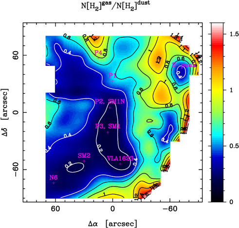
Figure 10: Gas-to-dust ratio map of $\rho$ Oph A calculated as the $\mathrm{H_{2}}$ column density from $\mathrm{C^{18}O}$ relative to the $\mathrm{H_{2}}$ column density from dust. The gas column data are based on the $\mathrm{C^{18}O}$(3-2) map of Liseau et al. (2010) and the dust continuum data are from Motte et al. (1998). The gas column data have not been corrected for opacity.

The freeze-out of CO on grains (together with low temperatures) is thought to increase the deuterium fractionation. Although the D-peak at $(0\arcsec,-30\arcsec)$ is located in the part where the $N(\mathrm{H_{2}})^{\mathrm{gas}}/N(\mathrm{H_{2}})^{\mathrm{dust}}$ opacity corrected ratio is low $\sim 0.3-0.4$, we do not see any signs that CO depletion is in effect more at $(0\arcsec,-30\arcsec)$ than in any of the other central positions. Hence, the amount of CO depletion (at least as measured by the $\mathrm{C^{18}O}$ emission and the 1.3 mm continuum data) is not directly responsible to the elevated deuterium fractionation seen in formaldehyde toward the D-peak. However, the D-peak is located within a larger region that is likely to be depleted and this may have been important in an earlier stage of the evolution of the D-peak source.

Interestingly, there is a minimum in the $N(\mathrm{H_{2}})^{\mathrm{gas}}/N(\mathrm{H_{2}})^{\mathrm{dust}}$ ratio in the SE part of the map (Fig. 10). This minimum coincides with the secondary $\mathrm{N_{2}D^{+}}$ peak (N6). This would be in line with the findings that the amount of CO depletion and the $\mathrm{N_{2}D^{+}}$/$\mathrm{N_{2}H^{+}}$ ratio are correlated in starless cores (Crapsi et al. 2005). Moreover, the Class 0 source VLA 1623 is also associated with a minimum in the $N(\mathrm{H_{2}})^{\mathrm{gas}}/N(\mathrm{H_{2}})^{\mathrm{dust}}$ ratio and possibly also with a higher $\mathrm{N_{2}D^{+}}$/$\mathrm{N_{2}H^{+}}$ ratio, compare Fig. 9 and Fig. 10. A correlation between CO depletion and $\mathrm{N_{2}D^{+}}$/$\mathrm{N_{2}H^{+}}$ ratio has been found by Emprechtinger et al. (2009) toward several Class 0 objects.

5.3 Gas-phase chemistry models

Pure gas-phase chemistry can lead to elevated deuterium fractionations for $\mathrm{H_{2}CO}$. We have here adopted the low-metalicity (or depleted) model of Roueff et al. (2007) as their warm-core (and un-depleted) model shows low deuterium fractionations. The steady-state model work presented here includes the updates and modifications of Parise et al. (2009), and we have used it to predict relevant D/H ratios for $\mathrm{H_{2}CO}$ and $\mathrm{N_{2}H^{+}}$. The models are shown in Fig. 11. The different steady-state D/H model ratios are shown as a function of temperature and have been calculated for two different $\mathrm{H_{2}}$ densities; $5\times 10^{5}\,\mathrm{cm^{-3}}$ and $1\times 10^{6}\,\mathrm{cm^{-3}}$. The modelled ratios show little variation due to the used $\mathrm{H_{2}}$ density. The observed column density ratios (taken from Table 10 and Table 11) are represented as coloured boxes with size according to estimated uncertainty. The dashed rectangle indicates the $\mathrm{N_{2}D^{+}}$/$\mathrm{N_{2}H^{+}}$ ratio toward the D-peak with an opacity correction.

It is noteworthy that the gas-phase depleted models yield $F$-values, see Eq. (1), very close to 0.5 for $T\la 30\,\mathrm{K}$ for formaldehyde which are significantly higher than the observed values $F\approx 0.1$, cf. Table 10. The absolute $\mathrm{H_{2}CO}$ abundances, $(3-6)\times 10^{-11}$, for these models are much lower than the observed $\mathrm{H_{2}CO}$ abundances $\sim 5\times 10^{-9}$.

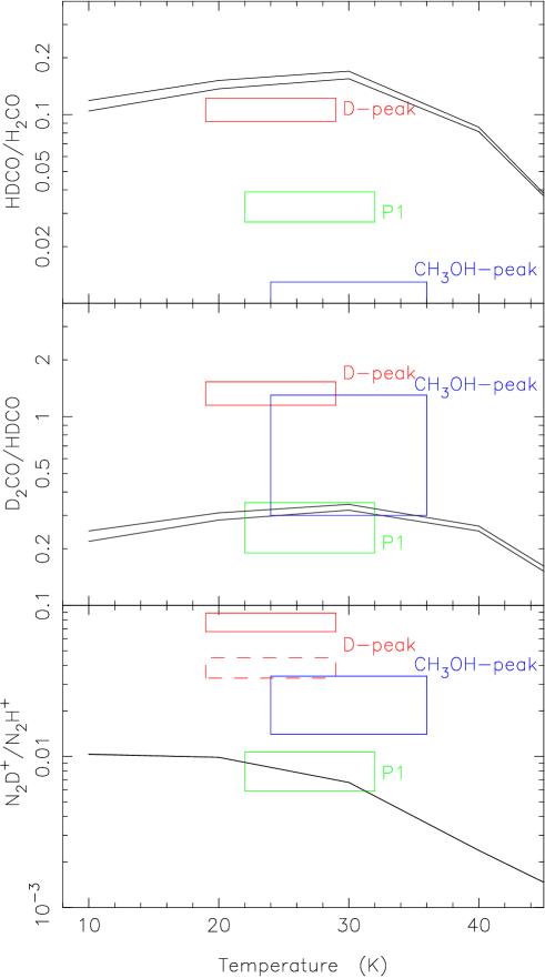
Figure 11: Gas-phase steady-state models based on the reaction network by Roueff et al. (2007). Shown are the D/H predicted ratios; $\mathrm{HDCO}$/$\mathrm{H_{2}CO}$ (top), $\mathrm{D_{2}CO}$/$\mathrm{HDCO}$ (middle), and $\mathrm{N_{2}D^{+}}$/$\mathrm{N_{2}H^{+}}$ (bottom) as function of temperature and for two different $\mathrm{H_{2}}$ densities ($5\times 10^{5}\,\mathrm{cm^{-3}}$ and $1\times 10^{6}\,\mathrm{cm^{-3}}$). The coloured boxes correspond to the observed ratios for the three cores as indicated in the top panel. The size of the rectangles represents the estimated uncertainties.

5.4 Grain chemistry models

Our observations point to the fact that $\mathrm{D_{2}CO}$ is more abundant than $\mathrm{HDCO}$ toward the D-peak. This is, to our knowledge, the first source where such case is observed. We note that $\mathrm{HDCO}$ and $\mathrm{H_{2}CO}$ showed a similar anomaly towards L1527 (Parise et al. 2006), but even in that case, $\mathrm{D_{2}CO}$ was less abundant than $\mathrm{HDCO}$. This anomaly is difficult to explain in terms of pure gas-phase chemistry, as discussed above.

We discuss here the possibility that this anomaly stems from grain chemistry. Simple grain models which only account for H and D additions to CO to form formaldehyde and methanol cannot account for enrichment of $\mathrm{D_{2}CO}$ compared to the statistically expected value. However, including the abstraction or exchange reactions of the type $\mathrm{HDCO+H\to DCO+H_{2}}$, Rodgers & Charnley (2002) argue that the enrichment is anyway limited to $\mathrm{HDCO}$/$\mathrm{H_{2}CO}$ $>$ $\mathrm{D_{2}CO}$/$\mathrm{HDCO}$ (or $F>1$, see Eq. (1)). Our observational results (with $F\approx 0.1$), as well as those of Parise et al. (2006) and Roberts & Millar (2007), are contradictory to this model prediction, showing that even this detailed model may be lacking some processes.

Some laboratory experiments have aimed in the last years to explain the large fractionations of formaldehyde and methanol observed towards low-mass protostars. Different types of experiments have been done (see Watanabe & Kouchi 2008, for an overview). Nagaoka et al. (2005) have exposed CO ices with H and D atoms (with D/H of 0.1) and have shown that $\mathrm{H_{2}CO}$ and $\mathrm{CH_{3}OH}$ (as well as their deuterated counterparts) are formed. In this experiment, they can reproduce the fractionation of all deuterated methanol molecules observed towards IRAS16293$-$2442 (Parise et al. 2004). However, they never observe an enrichment of $\mathrm{D_{2}CO}$ higher than $\mathrm{HDCO}$ (Naoki Watanabe, priv. comm.). In a second type of experiment, Hidaka et al. (2009) aimed at clarifying the different formation routes by exposing an $\mathrm{H_{2}CO}$ ice sample with D atoms. Exchanges are observed, showing that deuterium fractionation occurs very efficiently along the reaction path $\mathrm{H_{2}CO\to HDCO\to D_{2}CO}$. In this case, the observed $\mathrm{D_{2}CO}$ can become more abundant than $\mathrm{HDCO}$ (see their Figure 3). Although a direct extrapolation from these experiments is difficult, our observations may be the definitive evidence that abstraction and exchange reactions are playing an important role in grain chemistry. It is not clear if reproducing our observations will require an increased atomic D/H ratio (from the 0.1 value used by Nagaoka et al. 2005) incoming on the grains, or if the longer timescales involved in the ISM chemistry compared to the laboratory experiments also can play a role. Detailed modelling of the complex processes taking place on the grains would be needed to definitely settle this question.

There is no known central source towards the D-peak. So, unlike the case of IRAS16293$-$2422, there is no protostar that can be responsible for releasing the deuterated material into the gas. We therefore need to invoke heating of the grains by cosmic rays (e.g. Herbst & Cuppen 2006) or through the release of the formation energy of the newly formed species (Garrod et al. 2006). Both these mechanisms can be of importance for desorption of grain mantles in starless cores. However, even if these mechanisms are responsible of releasing the deuterated material into the gas, there is no obvious reason why they would be more effective in the SM1 core as compared to the other cores. Hence, the underlying question why the D-peak shows such a high deuterium fractionation remains unanswered.

6 Conclusions

We have observed a very high degree of deuteration of formaldehyde towards a core (SM1) in $\rho$ Oph A. In this D-peak, the deuterium fractionation manifests itself by a very high $\mathrm{D_{2}CO}$/$\mathrm{HDCO}$ ratio of $1.34\pm 0.19$ while the ratio $\mathrm{HDCO}$/$\mathrm{H_{2}CO}$ is $0.107\pm 0.015$. In the other parts of this cloud core the degree of deuteration in formaldehyde is much lower (although still very high compared to the ISM D/H ratio). For instance, at the P1 position, about $1^{\prime}$ (or 0.035 pc) north of the D-peak, the corresponding ratios are $0.27\pm 0.08$ and $0.033\pm 0.006$, respectively. A similar decrease in deuterium fractionation between the two positions is also seen for $\mathrm{N_{2}D^{+}}$/$\mathrm{N_{2}H^{+}}$. The $\mathrm{H_{2}CO}$ abundance relative to $\mathrm{H_{2}}$ is estimated to be around $5\times 10^{-9}$ over the central core.

The $\mathrm{CH_{3}OH}$ distribution is clearly different from that of $\mathrm{H_{2}CO}$ and it has its maximum about $45^{\prime\prime}$ to the northwest of the deuterium peak. The elevated methanol abundance (by about a factor of 5 relative to the D-peak) here could be due to an interaction of the outflow with a dense clump. It would be interesting to study how the deuterated versions of $\mathrm{CH_{3}OH}$ are distributed in this source (cf. Parise et al. 2006).

In order to understand the reason of the very high deuteration level observed toward the D-peak we have performed gas-phase chemistry modelling (for a depleted source). By looking at the ratio ($\mathrm{HDCO}$/$\mathrm{H_{2}CO}$)/($\mathrm{D_{2}CO}$/$\mathrm{HDCO}$) (the $F$-value, see Eq. (1)) we find that the models result in values around 0.5 while the observed values are always around 0.1. Also, the absolute $\mathrm{H_{2}CO}$ abundances obtained in these models are too low by a factor of 100. Hence, the gas-phase chemistry scheme cannot account for the observed $\mathrm{H_{2}CO}$ abundances and deuterium ratios. Instead, we advocate that grain chemistry, in terms of abstraction and exchange reactions in the reaction chain $\mathrm{H_{2}CO\to HDCO\to D_{2}CO}$ (Hidaka et al. 2009), can be responsible for the very high deuterium fractionations observed in $\rho$ Oph A. However, before being too conclusive about, e.g., the required atomic D/H ratio, these grain chemistry model results need to be expressed in observable quantities like the $\mathrm{H_{2}CO}$ $F$-value. Again, observations of multiply deuterated methanol isotopologues toward the D-peak in $\rho$ Oph A will provide additional insight as they are key ingredients in the grain chemistry scheme.