Mobility and Diffusion of a Tagged Particle in a Driven Colloidal Suspension

Abstract

We study numerically the influence of density and strain rate on the diffusion and mobility of a single tagged particle in a sheared colloidal suspension. We determine independently the time-dependent velocity autocorrelation functions and, through a novel method, the response functions with respect to a small force. While both the diffusion coefficient and the mobility depend on the strain rate the latter exhibits a rather weak dependency. Somewhat surprisingly, we find that the initial decay of response and correlation functions coincide, allowing for an interpretation in terms of an ’effective temperature’. Such a phenomenological effective temperature recovers the Einstein relation in nonequilibrium. We show that our data is well described by two expansions to lowest order in the strain rate.

1 Introduction

The mobility of a single spherical particle immersed in a solvent determines the velocity of the particle in response to an applied external force. For small Reynolds numbers Stokes’ law yields the famous expression $\mu_{0}^{-1}=3\pi\eta a$ in terms of the sphere diameter $a$ and the solvent viscosity $\eta$ in thermal equilibrium. This free mobility $\mu_{0}$ is intimately related to spontaneous solvent fluctuations through the Einstein relation. For a suspension of interacting particles, even without hydrodynamic coupling, the mobility $\mu$ of a single tagged particle is reduced. This reflects the fact that work is necessary to displace neighboring particles in order for the tagged particle to move, leading to larger dissipation. Still, in equilibrium the Einstein relation

$$D=k_{\text{B}}T\mu$$ (1)

equates the effective, long-time diffusion coefficient $D$ obtained from measuring the mean square displacement of a single tagged particle with its mobility through the solvent temperature $T$, where $k_{\text{B}}$ is the Boltzmann constant.

The Einstein relation (1) is one out of many fluctuation-dissipation relations valid in the linear response regime for small perturbations of the equilibrium state [1]. It is crucial to realize that also nonequilibrium steady states allow for a linear response. However, driving the suspension beyond the linear response regime, fluctuation-dissipation relations such as the Einstein relation (1) need to be generalized to nonequilibrium. There are two basic strategies discussed in the literature. The first strategy is to introduce an additive correction taking on the form of another correlation function [2, 3, 4]. This correlation function involves another observable that can be related either to entropy production [5] or ’dynamical activity’ [6]. Such an approach has been demonstrated experimentally for a single driven colloidal particle [7, 8, 9]. The second strategy introduces a multiplicative correction through an effective temperature [10, 11] replacing $T$ in Eq. (1). Originally developed in the context of aging, glassy dynamics and weakly driven systems, effective temperatures have also been investigated in shear driven supercooled liquids [12].

Self-diffusion in sheared interacting suspensions has been studied extensively in computer simulations [13, 14, 15, 16, 12] and experiments [17, 18] as well as analytically [19, 20, 21]. A large body of publications studies supercooled conditions in relation with the glass transition [12, 18, 22]. Most of these works focus on the self-diffusion coefficient as this quantity is easily obtained from experiments and simulations. The mobility of a tagged particle has been addressed somewhat less prominently and mostly in analytic calculations [23, 21]. In this Letter we determine numerically both the full time-dependent velocity response and autocorrelation functions for a tagged particle of a hard-core Yukawa suspension driven into a nonequilibrium steady state through simple shear flow. In contrast to previous work, explicit knowledge of the response function allows us to calculate and discuss the mobility as a function of density and strain rate. We use a novel method to efficiently obtain the time-dependent response function of the velocity with respect to a small force applied to a single particle. Similar methods to extract the response of a system using only unperturbed steady state trajectories have been discussed in Refs. [24, 25].

2 Sheared hard-core Yukawa fluid

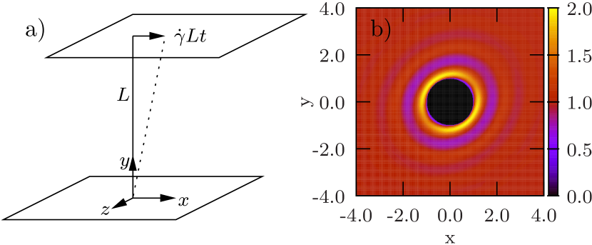
Figure 1: a) Simple shear flow with strain rate $\dot{\gamma}$. b) Pair distribution function $g(\mathbf{r})$ in the $xy$ plane for volume fraction $\phi=0.3$ and strain rate $\dot{\gamma}=1$. Centered on any particle, the function $g(\mathbf{r})$ quantifies the probability to find another particle at $\mathbf{r}$. While isotropic in equilibrium, the pair distribution function is distorted through external flow.

The $N$ colloidal particles interact through the purely repulsive Yukawa potential

$$u(r)=\begin{cases}\varepsilon\frac{e^{-\kappa(r-1)}}{r}&(r\geqslant 1)\\ \infty&(r<1)\end{cases}$$ (2)

with hard core exclusion. The two potential parameters are the energy $\varepsilon$ at contact and the screening length $\kappa^{-1}$ determining the range of interactions. Changing $\kappa$ interpolates between hard-sphere (large $\kappa$) and coulombic (small $\kappa$) interactions. Throughout the paper we employ dimensionless units and measure length in units of the particle diameter $a$ and energies in units of $k_{\text{B}}T$. The time scale $3\pi a^{3}\eta/k_{\text{B}}T$ is set by the time a particle diffuses a distance equal to its diameter. In particular, employing these units the mobility and diffusion coefficient of a free particle reduce to unity, $D_{0}=\mu_{0}=1$. We set $\kappa^{-1}=0.2$ and choose $\varepsilon=8$ such that the liquid is stable for a large pressure range [26]. We explore the liquid phase at four volume fractions $\phi\equiv 0.1,0.2,0.3,0.4$, where $\phi=\pi N(a/L)^{3}/6$ with $L$ the side length of the cubic simulation box. The highest density $\phi=0.4$ is close to the equilibrium freezing transition, which occurs at a pressure $28.9$ [26] (for $\phi=0.4$ the measured pressure in our simulation is $27.6$). For comparison, the freezing transition in a hard sphere suspension occurs at $\phi\simeq 0.494$ [27].

We employ Brownian dynamics simulations, for details see the appendix. The suspension is driven into a nonequilibrium steady state through simple shear flow $\mathbf{u}(\mathbf{r})=\dot{\gamma}y\mathbf{e}_{x}$ with strain rate $\dot{\gamma}$ (which equals the Péclet number in our units), see Fig. 1a). The equations of motion are $\dot{\mathbf{r}}_{k}=\mathbf{v}^{0}_{k}$ and

$$\dot{\mathbf{v}}^{0}_{k}=-\nabla_{k}U-[\mathbf{v}^{0}_{k}-\mathbf{u}(\mathbf{r}_{k})]+\mathbf{f}_{k}+\boldsymbol{\xi}_{k},$$ (3)

where the dimensionless mass is set to one. Physically, this choice implies that momenta relax on the diffusive time scale. Besides the forces due to the potential energy $U\equiv\sum_{k<k^{\prime}}u(|\mathbf{r}_{k}-\mathbf{r}_{k^{\prime}}|)$ we allow for direct forces $\mathbf{f}_{k}$. The stochastic noise $\boldsymbol{\xi}_{k}$ modeling the interactions with the solvent has zero mean and correlations $\langle\xi_{ki}(t)\xi_{k^{\prime}j}(t^{\prime})\rangle=2\delta_{ij}\delta_{kk^{\prime}}\delta(t-t^{\prime})$, where $i,j=x,y,z$ is the vector component. In Eq. (3), we neglect hydrodynamic coupling between different particles due to the solvent.

For the shear flow turned on we correct the particle velocities $\{\mathbf{v}^{0}_{k}\}$ by the external flow and investigate the relative velocity $\mathbf{v}_{k}=\mathbf{v}^{0}_{k}-\mathbf{u}(\mathbf{r}_{k})$. We are interested in the dynamics of a single tagged particle interacting with the remaining $N-1$ particles in the suspension. Since all particles are identical we designate particle 1 as the tagged particle and drop the subscript; in the following $\mathbf{r}$ and $\mathbf{v}$ are the position and relative velocity of the tagged particle, respectively. We define the response of this velocity

$$R_{ij}(t-t^{\prime};\dot{\gamma})\equiv\frac{\delta\langle v_{i}(t)\rangle}{\delta f_{j}(t^{\prime})}$$ (4)

with respect to an additional small force $\mathbf{f}$. In addition, we define the relative velocity autocorrelation matrix

$$C_{ij}(t-t^{\prime};\dot{\gamma})\equiv\langle v_{i}(t)v_{j}(t^{\prime})\rangle_{0}.$$ (5)

The brackets $\langle\cdots\rangle_{0}$ refer to an average with respect to the unperturbed steady state whereas $\langle\cdot\rangle$ is the average with the external force applied. In equilibrium ($\dot{\gamma}=0$) the fluctuation-dissipation theorem $R_{ij}(t)=C_{ij}(t)$ holds.

3 Response function

Sampling the correlation function (5) is straightforward. The direct way to obtain the response matrix (4) from simulations would be through a step perturbation of the force and the subsequent recording of the tagged particle’s velocity. Such a protocol has to be repeated many times and the corresponding response function follows as the time-derivative of the mean velocity. Here, we follow another route and determine the response function through the path integral representation of the fluctuation-dissipation theorem (FDT) for nonequilibrium steady states. The FDT in its general form reads

$$R_{ij}(t-t^{\prime};\dot{\gamma})=\langle v_{i}(t)B_{j}(t^{\prime})\rangle_{0}$$

with observable $B_{j}(t)=\delta\ln P/\delta f_{j}(t)|_{\mathbf{f}=0}$ conjugate to the perturbation force $\mathbf{f}$ acting on the tagged particle. The stochastic path weight is

$$P[\{\boldsymbol{\xi}_{k}(t)\};\mathbf{f}(t)]=\mathcal{N}\exp\left\{-\frac{1}{4}\sum_{k=1}^{N}\int\mathrm{d}t\;\boldsymbol{\xi}^{2}_{k}(t)\right\}$$

with normalization constant $\mathcal{N}$. From Eq. (3) we see that a perturbation of $\mathbf{f}$ is equivalent to a perturbation of $\boldsymbol{\xi}$ with $\delta\xi_{i}(t)/\delta f_{j}(t^{\prime})=-\delta_{ij}\delta(t-t^{\prime})$ we immediately obtain $B_{j}=\xi_{j}/2$ and therefore

$$R_{ij}(t-t^{\prime};\dot{\gamma})=\frac{1}{2}\langle v_{i}(t)\xi_{j}(t^{\prime})\rangle_{0}.$$ (6)

Since in a computer simulation we have direct access to the noise we can exploit such an expression to obtain the response function through a steady state correlation function. While Eq. (6) has been known before [28, 4], to the best of our knowledge so far it has not been exploited to obtain the response function numerically.

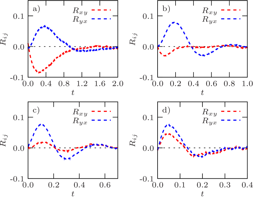
Figure 2: Comparison of the off-diagonal components $R_{xy}(t)$ and $R_{yx}(t)$ for strain rate $\dot{\gamma}=1.0$ and the four simulated volume fractions: a) $\phi=0.1$, b) $\phi=0.2$, c) $\phi=0.3$, and d) $\phi=0.4$. Increasing the density, the two curves approach each other until for the highest density they almost lie on top of each other. Note the changing time scale.

To understand the influence of the shear flow on the particle motion it is instructive to look at the off-diagonal components $R_{xy}$ and $R_{yx}$ plotted in Fig. 2. The component $R_{yx}$ describes the mean behavior of a tagged particle when we apply a force parallel to the shear flow and measure its velocity perpendicular in $y$ direction. The behavior of $R_{yx}$ can be explained by looking at the pair distribution function in Fig. 1b), which is deformed compared to its equilibrium isotropic shape. In order to move faster at short times the particle moves up ($R_{yx}$ is positive) to overcome its neighbors through a region of lower probability to encounter another particle. At a later time the particle is pushed back ($R_{yx}$ is negative) due to interactions with other particles which become more pronounced at higher densities. Interchanging $x$ and $y$-direction, the same arguments hold for the component $R_{xy}$. However, since we pull the particle up it enters a region where the surrounding fluid moves faster due to the shear flow. Hence, the particle is accelerated and the response of the relative velocity is negative for small times. With increasing density the particle cannot move far in $y$-direction, making the velocity differences smaller. The qualitative difference between the two curves diminishes and for $\phi=0.4$ both almost lie on top of each other. Hence, the effect of the shear flow on a single particle is more and more symmetric as particle motion becomes correlated at higher densities.

4 Diffusion and mobility

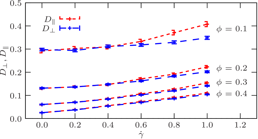
Figure 3: Diffusion coefficients $D_{\parallel}$ parallel and $D_{\perp}$ perpendicular to the shear flow vs. strain rate $\dot{\gamma}$ for the four different volume fractions $\phi$. For a free particle $D_{\perp}=D_{\parallel}=1$.

We now turn to the nonequilibrium diffusion coefficients and mobilities,

$$D_{ij}\equiv\int_{0}^{\infty}\mathrm{d}t\;C_{ij}(t),\quad\mu_{ij}\equiv\frac{\partial\langle v_{i}\rangle}{\partial f_{j}}=\int_{0}^{\infty}\mathrm{d}t\;R_{ij}(t),$$ (7)

which are obtained through integrating the velocity autocorrelation and response matrix, respectively. The mobility is defined as the velocity change in response to a small force applied to the tagged particle, perturbing the steady state reached through shearing the solvent. The diffusion coefficients are related to the velocity autocorrelation through a Green-Kubo kind relation. They are plotted in Fig. 3 and increase with increasing strain rate. From our data we find that we can distinguish diffusion parallel to the shear flow with $D_{\parallel}=D_{xx}$ and diffusion perpendicular with $D_{\perp}=D_{yy}=D_{zz}$. In shear flow the tagged particle moves between layers of different flow velocity effectively leading to larger fluctuations, allowing the particle to explore phase space faster. At low density the diffusion $D_{\parallel}$ parallel to the shear flow is substantially enhanced compared to $D_{\perp}$ even though we subtract out the external flow. However, the difference between the two diffusion coefficients vanishes with increasing density.

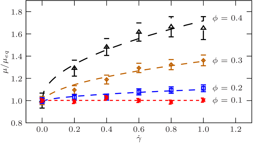
Figure 4: Reduced mobilities $\mu/\mu_{\text{eq}}$ vs. strain rate $\dot{\gamma}$ for the four different volume fractions $\phi$. The lines are fits to Eq. (8).

In Fig. 4 we plot the reduced mobility $\mu(\phi,\dot{\gamma})/\mu_{\text{eq}}(\phi)$ versus strain rate $\dot{\gamma}$ for the four simulated densities with equilibrium ($\dot{\gamma}=0$) mobility $\mu_{\text{eq}}$. We find that the diagonal components of the mobility matrix are equal within error bars and we obtain the shown mobilities through averaging over the three directions. The off-diagonal components are somewhat harder to obtain due to large statistical errors but are clearly much smaller than their diagonal counterparts (data not shown). The dependence of the absolute value of the mobility on the strain rate is rather weak and for the lowest density $\phi=0.1$ it is even constant. Such a weak dependence suggests that the ability of the solvent to reorganize in response to dragging the tagged particle out of the ’cage’ formed by neighboring particles is only slightly affected by the presence of the shear flow. Going to supercooled conditions, this is likely to break down [29].

To explain the dependence of the mobility on the strain rate we consider the mean velocity of the tagged particle from Eq. (3),

$$\langle\mathbf{v}\rangle=\langle\mathbf{F}^{(1)}\rangle+\mathbf{f}=-(N/L)^{3}\int\mathrm{d}\mathbf{r}\;g(\mathbf{r})\nabla u(\mathbf{r})+\mathbf{f}.$$

Here, $g(\mathbf{r};\phi,\dot{\gamma},\mathbf{f})$ is the pair distribution function to find a second particle at $\mathbf{r}$ if there is a particle at the origin, see Fig. 1b), and $\mathbf{F}^{(1)}\equiv-\nabla_{1}U$ is the force exerted by neighboring particles on the tagged particle. The effects of the shear flow and the force $\mathbf{f}$ enter only through the structure information encoded in the pair distribution function. We can expand $g$ into a Taylor series for small forces $\mathbf{f}$. On the other hand, it is well known that the structure of the suspension in the presence of shear flow is singularly perturbed from its isotropic equilibrium form [30, 31], requiring an asymptotic expansion in powers of $\dot{\gamma}^{1/2}$. Such an expansion in lowest order leads to

$$\mu(\phi,\dot{\gamma})\approx\mu_{\text{eq}}(\phi)\left[1+\chi(\phi)\dot{\gamma}^{1/2}\right].$$ (8)

In principle the coefficients $\chi(\phi)$ could be obtained from the knowledge of the perturbed pair distribution function $g(\mathbf{r})$. Here, we determine them through fitting the mobility, see the lines in Fig. 4. The fits show a good agreement with the simulated data for all strain rates and densities even though we have only retained the lowest order of the expansion (8).

5 Einstein relation

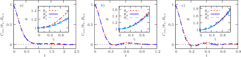
Figure 5: The response $R_{xx}(t)$ (dashed) and correlation $C_{xx}(t)$ (dotted) functions for volume fractions a) $\phi=0.1$, b) $\phi=0.2$, and c) $\phi=0.3$. The correlation functions are scaled by a constant factor $1/\theta_{x}$ to match the initial decay of the response function. The insets show these factors as a function of strain rate for the three directions, where the lines are fits to Eq. (9).

In Fig. 5 we plot $R_{xx}(t)$ and $C_{xx}(t)$ as functions of time for different volume fractions. The correlation functions have been scaled by a constant factor $1/\theta_{x}$ to match the initial decay of the response functions. This procedure reveals a rather good agreement between response and correlation function even for longer times (this holds also for the $yy$ and $zz$ components). We approximate the ratio

$$\frac{C_{ii}(t;\phi,\dot{\gamma})}{R_{ii}(t;\phi,\dot{\gamma})}\approx\theta_{i}(\phi,\dot{\gamma})\approx 1+\alpha_{i}(\phi)\dot{\gamma}^{2}$$ (9)

by these constant factors. Using $R_{ii}(0)=1$ we can interpret $\theta_{i}\approx\langle v_{i}^{2}\rangle_{0}$ as effective temperatures since they equal approximately the velocity fluctuations of the tagged particle. We have also checked the distribution functions of the velocity which are Gaussian with width $\sqrt{\theta_{i}}$ as expected.

In Eq. (9) we expand the correlation function to second order in the strain rate (due to the symmetry of simple shear flow there is no first order) with fit parameters $\alpha_{i}$. This expansion becomes exact in the case of interacting particles with linear forces [32]. In the insets of Fig. 5 the factors $\theta_{i}$ for the three directions $x$, $y$, and $z$ are shown to follow this quadratic prediction. Similar to the diffusion coefficients we can distinguish a factor $\theta_{\parallel}=\theta_{x}$ parallel, and a factor $\theta_{\perp}=\theta_{y}=\theta_{z}$ perpendicular to the shear flow. Again, increasing the density the difference between the two directions vanishes.

Two points are noteworthy. First, no simple proportionality can be found between the off-diagonal components of the response and the correlation matrix. Both have a qualitatively different shape (data not shown). In particular, the off-diagonal response components are strictly zero at $t=0$ whereas, in nonequilibrium, the off-diagonal velocity correlations are different from zero. Second, there is a fundamental difference compared to the effective temperature discussed for non-stationary, glassy dynamics out of equilibrium. There, fluctuation and dissipation are related by an effective temperature at low frequencies (i.e., on long time scales) while the initial decay of response and correlations is governed by the bath temperature [10]. Moreover, the effective temperature evolves slowly as the system approaches equilibrium. In contrast, in our case already the initial decay is governed by a temperature $\theta_{i}>1$. The effect of this temperature extends into the tails of response and correlation functions. It is only for high densities that we observe a deviation in the tails as can be seen in Fig. 5c).

We can finally write down a simple generalized Einstein relation

$$D_{ii}=\theta_{i}\mu$$ (10)

for the diagonal components of the diffusion matrix. Inserting the expansions for mobility [Eq. (8)] and effective temperature [Eq. (9)] we find that $D_{ii}-\mu_{\text{eq}}\sim\dot{\gamma}^{1/2}$ to lowest order. Such a dependence was also found in molecular dynamics simulations for a Lennard-Jones fluid [13, 14]. Due to the small $\chi/\alpha_{i}$ ratios we cannot resolve this $\dot{\gamma}^{1/2}$ dependence here.

In Fig. 6 we test the putative effective temperature by comparing $\theta_{\perp}\mu$ to the numerically obtained diffusion coefficient $D_{\perp}$ perpendicular to the shear flow. The mobility for $\phi=0.1$ is independent of strain rate and the diffusion follows the quadratic prediction $D_{\perp}\propto\dot{\gamma}^{2}$. While we find a good agreement for the two lowest densities, the effective temperature underestimates the diffusion coefficient at intermediate strain rates and high densities since the diffusion coefficient qualitatively changes and approaches a linear function $D_{\perp}\propto\dot{\gamma}$ at high densities. This indicates that the differences in the tails of response and velocity autocorrelation funtions become more important. Also, higher order terms might be required in the expansion of mobility and effective temperature.

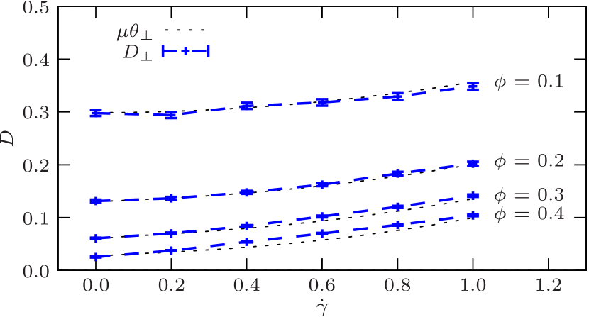
Figure 6: Test of the Einstein relation $D_{\perp}=\theta_{\perp}\mu$ with effective temperature $\theta_{\perp}$ from Eq. (9) and mobility from Eq. (8). The curves show a very good agreement for the lowest two densities but start to deviate at higher densities.

6 Experimental realization

We briefly discuss how our findings could be tested in experiments. Of course, the route via Eq. (6) to obtain the velocity response matrix through the explicit knowledge of the noise is not available in experiments. Moreover, the direct route, i.e. perturbing only a single particle within a suspension and measuring its time-dependent mean velocity, is experimentally challenging and, as we find in our simulations, also statistically more demanding.

Despite the difficulties it is still interesting to obtain this response function since it immediately yields the nonequilibrium mobility. We now assume that the tagged particle undergoes overdamped motion which is certainly the relevant limit for experiments. The Langevin equation for the tagged particle reads

$$\dot{\mathbf{r}}-\dot{\gamma}y\mathbf{e}_{x}=\mathbf{F}^{(1)}+\mathbf{f}+\boldsymbol{\xi}.$$ (11)

The replacement of the noise in Eq. (6) by Eq. (11) is permissible since the Jacobian arising due to the change of variables is independent of $\mathbf{f}$. We then obtain an experimentally accessible expression for the response function

$$R_{ij}(t)=\frac{1}{2}\left[C_{ij}(t)-\langle v_{i}(t)F^{(1)}_{j}(0)\rangle_{0}\right]$$ (12)

for components $i,j=y,z$ perpendicular to the shear flow. Let us assume that we record the particle position $\mathbf{r}_{k}$ at times $t_{k}\equiv k\tau$ with time resolution $\tau$, e.g., through video microscopy. The velocity is then approximated through the finite difference $\mathbf{v}_{k}=(\mathbf{r}_{k}-\mathbf{r}_{k-1})/\tau$. In principle, the force $\mathbf{F}^{(1)}$ on the tagged particle can be calculated from the knowledge of the pair potential and the positions of all neighboring particles.

7 Conclusions

We have studied a hard-core Yukawa colloidal system at different densities driven into a nonequilibrium steady state through shear flow. In particular, we investigate diffusion and mobility of a single tagged particle for four volume fractions $\phi$ and intermediate strain rates $\dot{\gamma}\leqslant 1$. The self-diffusion coefficient is calculated through the Green-Kubo relation from the single particle’s velocity autocorrelation function. The mobility is obtained from the particle’s response function through integration. For systems governed by stochastic dynamics, this response function can be obtained efficiently from the correlation function Eq. (6) measured in the unperturbed steady state. While for low densities we can clearly distinguish quantities measured parallel and perpendicular to the shear flow, this difference vanishes for high densities.

Surprisingly, the diagonal components of the response (i.e., the response is measured in the direction of the applied force) and correlation matrix can be matched over a large time range. The resulting proportionality factor can be interpreted as an effective temperature, effectively restoring the Einstein relation connecting diffusion and mobility. Moreover, this proportionality factor is well approximated by a quadratic expansion in the strain rate. It will be important to study how general such a simple effective temperature is for driven interacting colloidal suspensions and whether it extends to other observables. We believe that the methodology presented here will lead to new insights in the numerical study of dense colloidal suspension, e.g., for microscopic stress fluctuations [32, 35]. Finally, the influence of hydrodynamic interactions on our results remains to be investigated.

8 Appendix: Simulation details

The simulated systems consist of $N=1728$ particles in a cubic simulation box. Since we are interested in the bulk behavior of the suspension we employ periodic boundary conditions and account for the shear flow through Lees-Edwards sliding bricks. The equations of motion are integrated by a stochastic version of the velocity Verlet algorithm [33], where the velocity appearing in the force term at the right hand side of Eq. (3) is taken from the mid-step velocity. The time step is set to $\Delta t=0.0005\ll(\kappa\sqrt{\langle v_{i}^{2}\rangle})^{-1}\sim 0.08\dots 0.2$. We equilibrate the suspension and then slowly increase the strain rate to the final value. Correlation functions have been obtained by averaging over 400 particle trajectories with 300,000 time steps each. These trajectories have been determined in two independent runs from randomly chosen particles.

To implement the hard-core repulsion and prevent particles from overlapping, the following simple algorithm is employed (see also Refs. [34, 16] and references therein). After every particle has been moved, but before new forces are calculated, we store all overlapping particle pairs and remove these overlaps as follows. For each pair both of the particles are moved backwards in time along their respective velocity vector up to the point where they collided. This time $0<s<\Delta t$ is stored. Knowing the positions and velocities at the impact, we compute the connection vector $\mathbf{e}$ between both particles. We decompose the velocities into $\mathbf{v}_{1,2}^{\parallel}=\mathbf{e}\mathbf{e}^{T}\mathbf{v}_{1,2}$ and $\mathbf{v}_{1,2}^{\perp}=(\mathbf{1}-\mathbf{e}\mathbf{e}^{T})\mathbf{v}_{1,2}$. Only the parts parallel to $\mathbf{e}$ can change. Using the usual elastic collision rule preserving momentum and kinetic energy of the particles we obtain the after-collision velocities $\mathbf{v}_{1}^{\prime}=\mathbf{v}_{1}^{\perp}+\mathbf{v}_{2}^{\parallel}$ and $\mathbf{v}_{2}^{\prime}=\mathbf{v}_{2}^{\perp}+\mathbf{v}_{1}^{\parallel}$. From the positions of their collision the particles are then propagated forward with time step $s$ along the new velocity vectors. This procedure is repeated as long as overlapping pairs exist.

References

- [1] R. Kubo, M. Toda, and N. Hashitsume, Statistical Physics II, 2nd ed. (Springer-Verlag, Berlin, 1991).
- [2] A. Crisanti and F. Ritort, J. Phys. A: Math. Gen. 36, R181 (2003).
- [3] G. Diezemann, Phys. Rev. E 72, 011104 (2005).
- [4] T. Speck and U. Seifert, Europhys. Lett. 74, 391 (2006).
- [5] U. Seifert and T. Speck, EPL 89, 10007 (2010).
- [6] M. Baiesi, C. Maes, and B. Wynants, Phys. Rev. Lett. 103, 010602 (2009).
- [7] V. Blickle et al., Phys. Rev. Lett. 98, 210601 (2007).
- [8] J. R. Gomez-Solano et al., Phys. Rev. Lett. 103, 040601 (2009).
- [9] J. Mehl, V. Blickle, U. Seifert, and C. Bechinger, Phys. Rev. E 82, 032401 (2010).
- [10] L. F. Cugliandolo, J. Kurchan, and L. Peliti, Phys. Rev. E 55, 3898 (1997).
- [11] J. Kurchan, Nature 433, 222 (2005).
- [12] L. Berthier and J. Barrat, Phys. Rev. Lett. 89, 095702 (2002).
- [13] D. M. Heyes, J. Chem. Phys. 85, 997 (1986).
- [14] P. T. Cummings, B. Y. Wang, D. J. Evans, and K. J. Fraser, J. Chem. Phys. 94, 2149 (1991).
- [15] S. R. Rastogi, N. J. Wagner, and S. R. Lustig, J. Chem. Phys. 104, 9234 (1996).
- [16] D. R. Foss and J. F. Brady, J. Rheol. 44, 629 (2000).
- [17] X. Qiu et al., Phys. Rev. Lett. 61, 2554 (1988).
- [18] R. Besseling et al., Phys. Rev. Lett. 99, 028301 (2007).
- [19] A. V. Indrani and S. Ramaswamy, Phys. Rev. E 52, 6492 (1995).
- [20] J. F. Morris and J. F. Brady, J. Fluid Mech. 312, 223 (1996).
- [21] G. Szamel, Phys. Rev. Lett. 93, 178301 (2004).
- [22] M. Krüger and M. Fuchs, Prog. Theor. Phys. Suppl. 184, 172 (2010).
- [23] J. Bławzdziewicz and M. L. Ekiel-Jeżewska, Phys. Rev. E 51, 4704 (1995).
- [24] C. Chatelain, J. Stat. Mech. P06006 (2004).
- [25] L. Berthier, Phys. Rev. Lett. 98, 220601 (2007).
- [26] F. E. Azhar, M. Baus, J.-P. Ryckaert, and E. J. Meijer, J. Chem. Phys. 112, 5121 (2000).
- [27] V. J. Anderson and H. N. W. Lekkerkerker, Nature 416, 811 (2002).
- [28] P. Calabrese and A. Gambassi, J. Phys. A: Math. Gen. 38, R133 (2005).
- [29] P. Habdas et al., Europhys. Lett. 67, 477 (2004).
- [30] J. K. G. Dhont, An Introduction to Dynamics of Colloids (Elsevier, Amsterdam, 1996).
- [31] W. B. Russel, D. A. Saville, and W. R. Schowalter, Colloidal Dispersions (Cambridge University Press, Cambridge, 1995).
- [32] T. Speck and U. Seifert, Phys. Rev. E 79, 040102 (2009).
- [33] D. Frenkel and B. Smit, Understanding Molecular Simulation (Academic Press, San Diego, 2002).
- [34] P. Strating, Phys. Rev. E 59, 2175 (1999).
- [35] J. Zausch and J. Horbach, EPL 88, 60001 (2009).