Precision photometric monitoring of very low mass $\sigma$ Orionis cluster members: variability and rotation at a few Myr

Abstract

We present high-precision photometry on 107 variable low-mass stars and brown dwarfs in the $\sim$3 Myr $\sigma$ Orionis open cluster. We have carried out $I$-band photometric monitoring within two fields, encompassing 153 confirmed or candidate members of the low-mass cluster population, from 0.02 to 0.5 $M_{\odot}$. We are sensitive to brightness changes on time scales from 10 minutes to two weeks with amplitudes as low as 0.004 magnitudes, and find variability on these time scales in nearly 70% of cluster members. We identify both periodic and aperiodic modes of variability, as well as semi-periodic rapid fading events that are not accounted for by the standard explanations of rotational modulation of surface features or accretion. We have incorporated both optical and infrared color data to uncover trends in variability with mass and circumstellar disks. While the data confirm that the lowest-mass objects ($M<0.2M_{\odot}$) rotate more rapidly than the 0.2–0.5$M_{\odot}$ members, they do not support a direct connection between rotation rate and the presence of a disk. Finally, we speculate on the origin of irregular variability in cluster members with no evidence for disks or accretion.

1. Introduction

Stars and brown dwarfs in the $\sim$1-15 Myr age range occupy a pivotal position in the stellar evolution sequence, characterized by emergence from molecular cloud birthplaces, ongoing dissipation of primordial circumstellar disks, and assembly of planet systems. The evolutionary stage also involves dramatic changes in internal structure as well as radius and angular momentum. Some circumstellar and stellar changes during this epoch are interconnected, through deposition of accreting material on the central object, as well as possible transfer of angular momentum to the surrounding disk. Although the physics governing these processes remains difficult to probe directly, accompanying photometric variability offers a valuable tracer of the prevalence of various underlying phenomena at work.

It has long been known that pre-main-sequence T Tauri stars with masses near solar exhibit variability on levels of $\sim$1-50% (Joy 1949). At visible and near-infrared wavelengths, prominent phenomena causing photometric variability include modulations of the stellar brightness by rotation of cool magnetic surface spots, sporadic flux variations due to accretion, extinction fluctuations due to clumpy circumstellar material, and eclipses by companions. Data derived from temporal variability studies complement single-epoch surveys of stellar populations spanning a range of spectral types and ages in nearby young clusters by contributing information on changes occurring much faster than the evolutionary time scale. Photometric monitoring campaigns have thus become an integral part of our toolbox in the investigation of young cluster members.

Among the most appreciated stellar parameters accessed through time series monitoring is the rotational angular momentum. For objects with periodic brightness changes that can be attributed to the passage of cool surface spots, photometric variability analyses yield rotation rates. Recent work has established the overall angular momentum trends from the pre-main-sequence (PMS) through ages of 500 Myr, as reviewed by Herbst et al. (2007), Bouvier (2007), and Scholz (2009). Of particular interest is the 1-10 Myr regime, which is the first opportunity to measure the cumulative effect of the formation process on rotation rates after the embedded phases of protostellar development. During these early stages, a large portion of the initial angular momentum is carried off by outflows and jets, and additional amounts subsequently may be deposited into surrounding disks via magnetic interaction with the central star. The growing census of young stars and brown dwarfs has allowed recent studies to probe rotation rates in a number of 1-10 Myr old clusters, including Chamaeleon I (Joergens et al. 2003), IC 348 (Cohen et al. 2004; Littlefair et al. 2005; Cieza & Baliber 2006), Taurus (Nguyen et al. 2009), the Orion Nebula Cluster (Stassun et al. 1999; Herbst et al. 2002), $\sigma$ Orionis (Scholz & Eislöffel 2004), $\epsilon$ Orionis (Scholz & Eislöffel 2005), NGC 2363 (Irwin et al. 2008), and NGC 2264 (Lamm et al. 2005).

Observations to date find that the majority of rotation rates at ages of a few Myr correspond to periods between 1 and 10 days, with a smaller population of slower rotators extending to periods of $\sim$25 days. In addition, the distribution appears to be highly mass-dependent: earlier than spectral type M2.5 (or $\sim$0.3–0.4 $M_{\odot}$, depending on the theoretical model used), typical rotation periods lie between $\sim$2 and 10 days, and in some cases display a bimodal distribution (Herbst et al. 2002; Lamm et al. 2005) However, where data is available at lower mass, the distribution peaks near 1–3 days and steadily declines toward longer periods (e.g., Cieza & Baliber 2007). At first glance the slow rotation rates are somewhat surprising, given that these stars are recently accreting material and still undergoing pre-main-sequence contraction. Stellar evolution theory alone predicts approximately an order of magnitude increase in angular velocity during the PMS phase, whereas rotation rate distributions in clusters of different age remain roughly constant out to $\sim$30 Myr (Irwin & Bouvier 2009). Current evidence suggests that at least among the higher mass objects, rotation rates are strongly linked to the presence or lack of a disk, as indicated by long-wavelength infrared excesses (Rebull et al. 2006; Cieza & Baliber 2007).

Despite the wealth of data, many open questions remain, which we will address in this work. The mechanism for removal of angular momentum during the protostar stages is not well understood, and the role of circumstellar disks in rotation rate regulation remains controversial among the low-mass stars at spectral type M2.5 and later (Stassun et al. 1999; Rebull 2001). Furthermore, the lower limit to rotation periods in young clusters is not well established. Photometric derivations of rotation rate or pulsation period are complicated by the variety of variable phenomena operating in young stars. Notably, aperiodic variability due to stochastic accretion can appear as a semi-periodic phenomenon when sampling is sparse or when hot spots produced by columns of accreting material produce transient signals at the period of rotation (Bouvier & Bertout 1989; Fernandez & Eiroa 1996; Herbst et al. 2007). A number of authors claim evidence for a pattern of faster rotation as masses decrease into the brown dwarf regime (Bailer-Jones & Mundt 2001; Zapatero Osorio et al. 2003; Rodríguez-Ledesma et al. 2009). In some cases, periods as short as a few hours are inferred for brown dwarfs (BDs) and very low mass stars (VLMSs), implying that they may be spinning at close to break-up velocity. Palla & Baraffe (2005) suggested that variability in these particular short-period objects may represent a completely different effect– pulsation powered by deuterium burning. Detection of this phenomenon is one motivation for our work.

We recently initiated a campaign to probe low-amplitude photometric variability on short ($\sim$1-hour) time scales, obtaining rotation periods and searching for pulsation among young BDs and VLMSs ($<0.1M_{\odot}$). In this paper, we present results of photometric monitoring on members of the $\sim$3 Myr (Sherry et al. 2008) cluster around $\sigma$ Orionis. At a distance of 440 pc (Sherry et al. 2008), spatial extent of $\sim$1 square degree, [Fe/H] of -0.02 (González Hernández et al. 2008), and low extinction ($E$($B$-$V$)=0.05; Lee 1968), the cluster is a convenient target for photometric and spectroscopic studies. Indeed, prior surveys have revealed a rich population of 338 confirmed members (Caballero 2008, and references therein), along with some $\sim$300 additional candidates from photometry, proper motions, and x-ray detections (e.g., Hernández et al. 2007; Lodieu et al. 2009; Sherry et al. 2004; Franciosini et al. 2006). Of particular interest to our pulsation search is that $\sigma$ Orionis is one of few young clusters with very low mass members claimed to exhibit periodic variability on time scales of 2-5 hours, as reported by Bailer-Jones & Mundt (2001); Zapatero Osorio et al. (2003), and Scholz & Eislöffel (2004). However, apart from the latter study which presented 23 periodic objects in the northern reaches of the cluster, no comprehensive variability studies have been carried out in the main portion of the cluster. A campaign by Caballero et al. (2004) resulted in the measurement of three rotation periods from a sample of 28 candidate brown dwarfs, while the studies by Bailer-Jones & Mundt (2001) and Zapatero Osorio et al. (2003) contributed another two. Other work by Hernández et al. (2007) and Lodieu et al. (2009) present evidence for generic variability based on sparsely sampled photometry over year time scales.

We have taken advantage of the numerous prior single-pointing surveys to select a sample of $\sim$150 likely young BDs and VLMSs distributed throughout $\sigma$ Orionis. We collected photometry on these objects with the Cerro Tololo Interamerican Observatory (CTIO) 1.0-meter telescope and Y4KCam detector, operated by the SMARTS consortium. We obtained data on two observing runs of nearly two weeks each, benefiting from uninterrupted clear skies and probing to magnitudes of $I$=21, well beyond the substellar boundary (I$\sim$17). The excellent precision of our dataset (a few percent or better for the majority of targets) and continuous monitoring offers an unprecedented window into low-amplitude variability on 15-minute to two-week time scales in VLMSs and BDs, encompassing multiple rotation periods for many of these objects. Based on these observations, we present 65 new rotation rates– more than tripling the number for confirmed and likely $\sigma$ Ori members– as well as provide a new assessment of the period distribution among late-type objects. In addition, we show evidence for other types of variability, including possible rapid circumstellar extinction events associated with very low mass stars. We identify several new candidate members of the cluster based on their variability and colors.

The outline for this paper is as follows: In $\S$2 and $\S 3$, we respectively describe the selection of photometric targets in $\sigma$ Orionis and basic data acquisition and reduction procedures. In $\S$4, we detail several different photometry techniques tested to minimize night-to-night photometric systematics and achieve the lowest possible noise scatter in our time series. In $\S$5 and $\S$6, we discuss our methods for identifying both periodic and aperiodic variability in the light curves, as well as the corresponding detection limits as a function of magnitude and frequency (in the case of periodic variability). In $\S$7, we present an overview of the types of variability found in our sample, as well as analyze the connections to parameters such as color, mass, time scale, and circumstellar disk indicators. Finally, in $\S$8, we present our main findings concerning young cluster variability in the context of prior studies. The Appendix includes a detailed list of all previously identified $\sigma$ Orionis variables that fall in our fields of view, along with redetections where applicable.

2. Target Fields

The $\sigma$ Orionis cluster was first identified by Wolk (1996) and Walter et al. (1997) via clustered sources of x-ray emission in ROSAT observations. Possibly associated with the Orion OB1b subgroup, the cluster of low-mass stars surrounds the O9.5V binary star $\sigma$ Ori AB. Béjar et al. (1999) and Zapatero Osorio et al. (2000) presented an initial sample of candidate low-mass cluster members, for most of which spectral types were later determined by Barrado y Navascués et al. (2003). Subsequent surveys (e.g., Sherry et al. 2004; Burningham et al. 2005; Kenyon et al. 2005) have augmented the list of low-mass candidate members via photometric selection in the near-IR, spectroscopic analysis of H$\alpha$, Na I, and Li lines, as well as characterization of mid-IR excesses indicative of disks (e.g., Hernández et al. 2007). While most of these methods do not rule out the presence of foreground and background sources, the contamination rate from photometry alone is expected to be relatively low ($\sim$15% based on the color-magnitude distribution of a non-cluster field; Lodieu et al. (2009)).

We compiled a list of likely and candidate $\sigma$ Orionis cluster members from Béjar et al. (1999), Béjar et al. (2001), Barrado y Navascués et al. (2001), Barrado y Navascués et al. (2003), Béjar et al. (2004), Caballero et al. (2004), Sherry et al. (2004), Scholz & Eislöffel (2004), Burningham et al. (2005), Kenyon et al. (2005), Franciosini et al. (2006), Caballero et al. (2007), Hernández et al. (2007), Caballero (2008), Luhman et al. (2008), and Lodieu et al. (2009), including available signatures of youth and kinematic measurements. Our observations target two fields (as shown in Fig. 4) selected to avoid bright stars such as $\sigma$ Ori AB itself, while maximizing both the density of confirmed or suspected low-mass cluster members and number of objects with previously observed variability. We cross-correlated the positions of objects in our fields with the above-mentioned sources to assemble a final list of confirmed and likely members appearing in our imaging data, which is provided in Table 1.

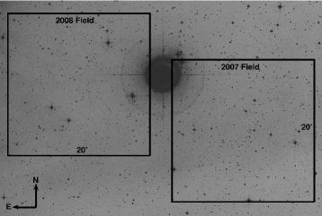
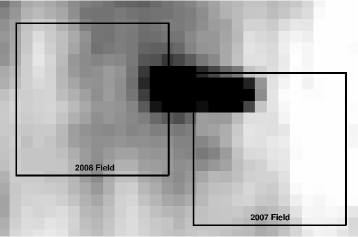
Figure 1.— Observed fields are superimposed on a Palomar Observatory Sky Survey 2 (POSS2) red image (top) obtained from the Digitized Sky Survey (DSS) and an Infrared Astronomical Satellite (IRAS) 100 $\mu$m image (bottom). The 2007 field is centered at RA=05^h38^m00.6^s and Dec=-02$\arcdeg$43$\arcmin$46.3$\arcsec$, while the coordinates of the 2008 field are RA=05^h39^m31.2^s, Dec=-02$\arcdeg$37$\arcmin$25.9$\arcsec$. $\sigma$ Ori itself is the bright object near center, and greater extinction is seen in the 2008 field than that from 2007.

3. Data Acquisition & Reduction

A field centered on RA=05^h38^m00.6^s and Dec=-02$\arcdeg$43$\arcmin$46.3$\arcsec$ in the $\sigma$ Orionis cluster was observed for 12 consecutive nights from 2007 December 27 to 2008 January 7 with the CTIO 1.0-m telescope and Y4KCam detector. A second field at RA=05^h39^m31.2^s, Dec=-02$\arcdeg$37$\arcmin$25.9$\arcsec$ was observed from 14 to 24 Dec 2008. During this second run, two repeat observations per night were also obtained of the first field, such that long-term photometric trends might be investigated. Skies were clear and photometric for the majority of observations, with little moon and seeing from 0.9$\arcsec$–1.8$\arcsec$. The CCD consists of a 4064$\times$4064 chip with 15 $\mu$m pixels, corresponding to a scale of 0.289$\arcsec$ pixel^-1 and an approximately 20$\arcmin\times$20$\arcmin$ field of view. Because readout occurs in quadrants, bias levels vary in the four regions. This effect unfortunately cannot be completely calibrated out, because both the mean bias level across the amplifiers as well as the two-dimensional spatial dependence are highly time variable, as seen in the behavior of the overscan region and bias images. Our photometry is largely unaffected by this issue since sky subtraction takes into account local bias levels around our targets. However, we have masked out data in the central 20 columns and rows of the CCD where rapid spatial variation in the bias between different quadrants prevents proper background extraction. The amplifiers have gains from 1.33 to 1.42 electron ADU^-1 and readout noise $\sim$7 electron pixel^-1.

The observations targeted 153 candidate very-low-mass $\sigma$ Ori members, including some 15 spectroscopically confirmed young brown dwarfs (see Table 1). Our goal of acquiring high-precision time series photometry on these objects required accumulation of as much signal as possible while maintaining an observing cadence well under the $\sim$1-hour time scales of interest for short-period signals. Theoretically, the shortest detectable sinusoidal period is twice the cadence; we elaborate on this relationship in §5. In practice, exposure times are limited by contamination from large numbers of cosmic ray hits and diffraction spikes from saturation of numerous nearby bright stars when count levels reach 50,000 ADU. As a compromise between these competing effects, we initially chose an exposure time of 360 seconds in the Cousins $I$ band, where the optical spectral energy distribution of brown dwarfs nears its maximum. During the 2008 observations, we increased integrations to 600 seconds for slightly improved signal-to-noise. Due to the consistent night-to-night observing conditions, these set-ups did not need to be adjusted throughout the runs. With a detector read-out time of 90 seconds in the unbinned mode, the resulting cadences were 7.5 and 11.5 minutes per photometric data point in the 2007 and 2008 run, respectively. The corresponding total observation times were 72 and 60 hours, resulting in 523 and 338 data points.

Careful calibration procedures were followed to ensure that the ultimate photometry was restricted mainly by source and sky background noise inherent to the measurements. Sets of bias images and dome flats were acquired daily. Since dome flat field images taken with the CTIO 1.0-m telescope are known to deviate from the true pixel sensitivity distribution by up to 10% toward the corners of the detector, we only used sky flat fields. Twilight sky flats were obtained at the beginning and end of each night in the $I$ band. Uniform bright sky illumination and detector response can be achieved with exposures of at least 10 seconds (to mitigate shutter shading effects) and less than a few minutes (to avoid the appearance of many stars in the flat field). Conditions allowed for four consecutive sky flats with flux levels averaging 30,000 counts, providing a good representation of pixel sensitivity variations within the linearity limit of the CCD. We checked that the combination of all eight twilight flats per night should contribute an uncertainty of less than 0.002 magnitudes per pixel to the photometry, sufficient for our precision requirements. For two nights when thin cirrus prevented uniform twilight exposures, we incorporated observations from adjoining nights into the composite flat field after confirming that the detector sensitivity did not change significantly over 24-hour time scales. In a few cases, new dust did appear on the CCD window midway through the night and its corresponding “donut” could not be adequately removed from the images. Affected areas were noted and confirmed not to lie in close proximity to any of our photometric targets or potential reference stars. We ensured that the pointing remained stable by choosing the same guide star from night to night and centering it in the same pixel of the guide camera.

We cleaned the images of cosmic rays with the IRAF cosmicrays utility. This detects and replaces sharp, non-stellar sources appearing more than five standard deviations above the background. Rare cosmic ray hits coincident with the stars and brown dwarfs are not removed in this way and must be identified separately in the later light curves. Standard reductions including subtraction of biases and flatfielding were carried out with the IRAF imred package. Images were split into quadrants, and each corrected with a high-order fit to its individual overscan, to account for highly variable bias structure at the edge between the bottom and top amplifiers. Quadrants were subsequently trimmed and pasted back together to form a seamless image. Residual two-dimensional bias structure was removed by subtracting a master frame of 20 median-combined zero images.

Because the $I$ band extends well beyond 8000$\AA$ and the typical CCD thickness is 20 $\mu$m or less, our images suffer from fringing, in which long-wavelength emission from OH night sky lines reflects multiple times within the CCD to create a complicated interference pattern superimposed on the images. An SDSS i filter, which better suppresses sky emission, was unavailable at the time of our observations. The fringing effect is additive and fixed with respect to detector position, but its strength varies throughout the night, depending on sky conditions. For the Y4KCam, we find that its amplitude typically fluctuates on scales of 30-50$\arcsec$, with amplitudes reaching 2% with respect to the background. While guiding generally keeps stars on the same pixel, steep gradients in the fringe pattern and an unexplained 4–5 pixel drift in $x$ position throughout the night could affect background subtraction for aperture photometry, introducing artificial variability on the same levels as potential rapid rotation or pulsation signatures. Hence we developed a procedure to effectively model and subtract the fringing from all images. Throughout the first run, we took 360-second exposures of sparsely populated areas of sky, amassing a total of 68 “fringe” flat fields. To isolate the fringe pattern in these images, it is important to extract the two-dimensional continuum sky background as well as stellar point sources. We generated object masks for each field, eliminating images with highly saturated stars. Because of varying bias levels in the different quadrants, we modeled the background to second order, allowing the fit to vary in each of the four regions. This piecewise background was then subtracted from each image, leaving a fringe pattern with mean value zero. A high signal-to-noise master fringe frame devoid of stars and background was created by median combining the individual fringe images, incorporating the object masks. To defringe an image, it is necessary to subtract the fringe frame scaled by the value determined to best reproduce the time-dependent fringe amplitude. The IRAF task rmfringe performed this process by iterating to minimize the difference between scaled fringe flat field and each background-subtracted, object-masked image. After a first round of fringe subtraction from the fringe fields themselves, we repeated these steps but instead used the processed images from the previous iteration to determine the sky background. This resulted in a slightly more accurate master fringe frame.

To defringe the two science fields in $\sigma$ Ori, we followed the same procedures, subtracting the scaled master fringe frame from the science images in two iterations. The second round again included input sky background as determined from the first round fringe-subtracted images. Since no fringe field exposures were taken during the 2008 run, we used the same 2007 master frame for this data, resulting in slightly higher residuals. We found that these steps effectively removed fringes in some 95% of images if liberal object masking was applied, especially in the northeast corner of the field where stray light from a bright nearby star reflected into the detector field of view. The remaining 5% of images were corrected by manual defringing. Fringe subtraction was successful in removing background variations down to the 0.1% level, suitable for our photometric purposes. Images were then aligned to the same $x$-$y$ coordinates with a small flux-preserving shift using the IRAF script IMAL2 provided by Deeg & Doyle (2001). This script takes as input a number of bright reference stars across an image, determines their centers using the IRAF imcentroid task, and outputs the mean shift in $x$ and $y$. It then uses the IRAF imshift task to perform the shift calculated for each image.

4. Photometry

The aim of our monitoring campaign is to obtain light curves with as high a cadence and precision as possible, thereby providing sensitivity to variability below the 0.01 magnitude level on sub-hour time scales. Optimizing signal-to-noise (S/N) ratios on the low-mass cluster targets in our fields is particularly challenging with a 1-meter telescope, as the selected 6 to 10-minute exposure times result in S/N=100 only on the brighter brown dwarfs in the sample. These exposures also lead to moderate numbers of cosmic ray hits as well as slightly non-symmetric psf shapes resulting from accumulated guiding errors. Consequently, we paid special attention to our photometric analysis procedures and tested several different routines to identify the one providing the best S/N performance.

4.1. Aperture Photometry

Since our fields are not particularly crowded, we expect aperture photometry to outperform point spread function (psf) fitting. We employed the IRAF script VAPHOT (based on phot; Deeg & Doyle 2001) to calculate instrumental magnitudes with apertures optimized to provide the best signal-to-noise ratios as a function of stellar flux, sky background, and seeing. Photometry of bright objects typically benefits from large apertures since the flux signal dominates over the background, while for faint objects smaller apertures are needed because photometric precision is sky-limited, as discussed by Howell (1989). Moreover, the optimal aperture size scales approximately with seeing, such that it is nearly constant when expressed as a multiple of the psf size. VAPHOT makes use of these properties to perform high-precision differential photometry without the need for multiple trials of different aperture sizes or aperture corrections. The program dynamically determines the best apertures for all desired photometric targets on a single input frame with seeing representative of the average for the entire run. The ratio of the calculated aperture sizes to the full width at half maximum (FWHM) of the psf is then fixed, and aperture sizes in all other frames are scaled relative to those determined for the chosen “typical” frame. All measurements on an object should thereby recover the same fraction of its total flux from frame to frame and night to night, in the limit that the psf is circularly symmetric. In reality, the psf is not perfectly symmetric, and this assumption introduces the need for a small correction to the measured fluxes. We have not applied such a correction here but discuss a method that we have used to reduce the error using image subtraction photometry in $\S$4.2.

Aperture photometry with the scaled aperture sizes was then carried out with the IRAF phot task, including redetermination of the object centroids before aperture placement. Typical aperture radii were 10.5 pixels ($\sim 3\arcsec$) for bright stars and 7 pixels ($\sim 2\arcsec$) for faint targets such as BDs. We do not perform aperture corrections since this introduces additional errors and our instrumental magnitudes differ from their flux-corrected counterparts by the same constant value, a situation entirely suitable for differential photometry. We have measured the sky background around each object within an annulus extending between 4.5 to 6 times the FWHM.

The primary difficulty we have encountered in producing high-precision photometry with VAPHOT is the implicit assumption of a psf fixed in both size across the image and in shape from night to night. The psf size across the Y4KCam detector is in fact known to vary by up to 25% from the center to corner. As provided, VAPHOT determines the seeing FWHM in each image by fitting a gaussian profile to a single bright star specified by the user. This value is then used to scale the apertures for all other objects in the field. We altered the script to instead output an average psf of several bright stars across the field. In addition, we found that the calculated optimal apertures for all but the faintest targets were too small, in that the aperture scaling based on psf size estimates introduced significant noise on night-to-night time scales. Doubling the aperture sizes for targets with $I<18$ reduced RMS spreads over the entire observing duration by more than 50% in most cases. Therefore, we adopted the larger aperture sizes for all object in the brighter half of our sample. These improvements confirm that neglecting spatial variations and non-gaussian shapes in the point spread function introduces substantial artificial variability in photometry with relatively small apertures.

Differential photometry was carried out with a suite of reference stars for which peak flux remained below the detector saturation and linearity limits on all nights. In each of the two fields, we selected an initial set of 10–20 bright (all I$\sim$13) reference stars, summed the fluxes in each image, and converted to a magnitude. Tests of several weighting schemes, such as the one suggested by Sokoloski et al. (2001) did not produce substantially different results. Differential magnitudes relative to this ensemble magnitude were computed for each of the reference stars in turn, with that particular star removed from the ensemble. We computed the light curve RMS values, and objects with variability visible by eye or RMS more than one standard deviation above the average RMS for that magnitude were removed from the ensemble. The process was repeated with the new subset of reference stars until no outliers remained. The final ensembles consisted of 4–6 reference stars, with spreads of $\sim$0.002 magnitudes over the course of the entire observing run. Based on this reference, differential light curves were generated for all objects in the field with signal below the saturation limit but at least five times the background.

A number of the light curves displayed significant zero-point changes on time scales of one or more days. These variations appeared even among some of the brightest targets but did not seem to occur systematically across all objects. We suspect that slow changes in the pointing and thus object mapping in $x$-$y$ pixel coordinates and other parameters such as seeing and airmass affect the photometry in a position-dependent way. To investigate associated trends in the light curves, we fit object magnitudes linearly as a function of psf FWHM and ellipticity, sky counts, object $x$ and $y$ position, relative centroid position, as well as airmass. The fit to most light curves was only weakly dependent on these parameters. Out of concern for unnecessary addition of noise to the data, we did not remove these low-level trends.

An additional consideration for the photometry is potential differences in color between the late-type objects in our sample and the brighter stars in the reference ensemble. To first order, extinction effects due to changing airmass cancel out in differential photometry. However, second-order color terms can introduce significant trends in the light curves if target objects are substantially redder than the reference ensemble (e.g., Young et al. 1991). Atmospheric extinction is weaker at longer wavelengths, and this can emerge as a gradual brightening of differential light curves for fainter, redder objects as airmass decreases. No such behavior is visible in the light curves of faint cluster members in our sample, and the absence of significant airmass-flux correlations confirms this finding. We suspect that the lack of obvious trends is due to the relatively weak dependence of extinction on wavelength beyond $\sim$ 7000$\AA$, as indicated by the small $I$-band color-dependent extinction coefficient determined later in $\S$4.3. Variable extinction due to changing atmospheric conditions could also produce artificial offsets in the object brightness, whereby the differential magnitudes would correlate with reference ensemble magnitude rather than airmass. Again, we fit the light curves for this effect, but did not detect significant trends and hence did not apply any corrections to the data.

The major sources of random error in the light curves are photon shot noise and sky background noise. We estimate based on the relation given by Young (1967) that atmospheric scintillation effects will introduce brightness fluctuations of less than 5$\times 10^{-4}$ magnitudes for the observational set-up here and hence should be negligible. To assess the quality of our light curves, we extracted photometry on all $\sim$3200 point sources identified in the fields and removed severely saturated objects from the sample. On time scales of less than one night, the floor of the distribution is well accounted for by photon and sky noise, plus an additional allowance of $\sim$0.002–0.0025 magnitudes in systematic error. The adopted uncertainty for our unbinned data range from 0.002 magnitudes for the bright reference stars, to just over 0.01 for the brown dwarfs near $I$=17, and 0.1 at the faint end where targets reach $I$=21. On the longer time scales corresponding to the observing duration, RMS light curve fluctuations are increased by up to 50% over these values because of night-to-night systematic effects.

4.2. Image Subtraction Photometry

Several concerns prompted us to perform an independent test of our results with a different set of photometric reduction procedures. For a few of the target brown dwarfs, flux from faint sources near our object apertures may have interfered with proper sky subtraction during aperture photometry. In addition, night-to-night variations in the mean magnitude of many sources suggests that spatial and temporal psf variations as well as slightly non-circular psf shape may be significant enough to alter the photometric zero point. Comparison tests of psf fitting photometry and image subtraction (e.g., Mochejska et al. 2002) have shown that the latter method can result in significantly smaller light curve scatter. Therefore, we opted to employ the method of differential image analysis (Alard & Lupton 1998; Mochejska et al. 2002) to produce a separate photometric dataset with reduced sensitivity to crowding and other psf effects. The Hotpants package (Becker et al. 2004) compares the fluxes of objects in every exposure to their counterparts in a selected reference image, thereby enabling a differential brightness measurement. Images are first accurately aligned to a common grid. A high-quality stacked reference image is then convolved with a time-dependent kernel which is mathematically optimized to reproduce the psf (size and shape) in all individual images. The science images are then subtracted from the convolved reference to reveal residuals possibly indicative of variability.

We found that subtraction from the reference template produced relatively clean images, with background consistent with the levels expected from noise properties of the input images. By specifying spatial variations of the background and psf kernel, we are able to obtain subtracted images devoid of systematic effects. Systematic residual flux is detectable above the background only in the brightest stars, where it appears in saturation-related peaks or a circular pattern with alternating positive and negative flux on either side. As pointed out by Alard & Lupton (1998), the latter pattern is likely the effect of small-scale atmospheric turbulence, which causes offsets of the psf centers even in well-aligned frames. We measured the residual flux in each subtracted image by performing nearly the same aperture photometry routines, as described in $\S$4.1. Inputs for aperture placement and size were determined from the convolved, unsubtracted images. To convert the measurements to differential magnitudes, we also measured fluxes of each star in the reference template, again using the same optimal aperture sizes determined by VAPHOT for the more standard photometry discussed in $\S$4.1. Magnitudes were then computed relative to the reference frame. For a selection of variables in which the signal dominated noise, we confirmed that the image subtraction routine produced the same light curves as the photometry performed on un-subtracted images, to within the photometric uncertainties. This technique is a hybrid version of the variable-aperture and image subtraction methods, the second of which typically involves an aperture correction even to compute the differential magnitude. Our approach thus eliminates important systematic noise contributions and should perform significantly better than either method alone.

We expect the photon and sky noise components of the image subtraction light curves to be similar to those derived from standard optimal aperture photometry. But since image subtraction photometry involves measurements on residuals (with at least an order of magnitude less flux, even for variable objects) resulting from the image subtraction optimization process, the light curves should be much less sensitive to errors in psf and aperture size. To test this assumption, we plot in Fig. 2 the RMS light curve spread as a function of magnitude over the duration of each observing run for the different photometry methods. We find that while doubling the aperture sizes (as explained in $\S$4.1) offers improvement in photometric precision in the standard optimal aperture method, image subtraction photometry indeed significantly outperforms both of these approaches. To assess each method in comparison with the expected uncertainties, we have estimated the poisson and sky noise components, based on the variable aperture size as a function of magnitude as well as the mean sky background value over all nights of each run. Apart from the brightest 3% of objects which are affected by our neglect of CCD non-linearity ($I\lesssim$14), the combination of image subtraction and optimal aperture selection produces light curves consistent with the analytically determined photon and sky noise floors plus a 0.002–0.0025 magnitude systematic uncertainty over the entirety of each run. These curves are shown in Fig. 2; they pass slightly below, as opposed to through the data distribution because of small systematics evidently unaccounted for in the sky background. Based on this assessment, we have adopted as our final dataset the image subtraction results for targets with $I>14$, and light curves from standard aperture photometry with double-sized apertures for $I<14$.

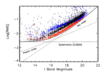
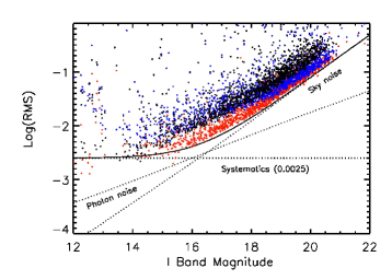
Figure 2.— Spread of photometry over the duration of each observing run, as a function of magnitude for three methods of variable-aperture photometry. The 2007 field is represented on the top, while the 2008 field is on the bottom. Blue dots represent photometry with the calculated optimal apertures, black dots are the same photometry with double-sized apertures, and red dots are the result of image subtraction followed by photometry with optimal-sized apertures. While the first two methods exhibit systematic errors particularly in the middle magnitude range, the trends for image subtraction photometry in both fields are well described by a combination of photon noise, sky background, and a small systematic contribution. Larger deviations at the bright end are due in part to CCD non-linearity. Points lying significantly above the trend signify variable objects or erroneous photometry (e.g., bad pixel or saturation effects) that was later removed.

4.3. Absolute Photometry & Colors

Because of the precision requirements of our observations, it was not efficient to observe standard fields frequently or collect multi-color data. Telescope motion compromises object pixel placement and thus introduces flat-fielding error effects. Filter changes are also associated with focus shifts and small position increments which often degrade data quality. However, standard magnitudes and color information can be very useful in distinguishing between the intrinsic properties of different variable sources. As a compromise, we obtained one or two $R$-band exposures of each $I$-band field every night. To derive the Cousins $R$ and $I$ magnitudes, we also observed a spatially dense Stetson photometric standard field in NGC 2818 at several different airmasses and performed aperture-corrected photometry on over 500 stars with available Stetson $R$ and $I$ magnitudes (Stetson 2000). The conversions from the CTIO filter (“r” and “i”) magnitudes was determined by fitting the following linear trends across a wide range of magnitudes and colors, as well as several airmass values ($X$):

$$I=i+(\epsilon_{I}+k_{I}^{{}^{\prime}}X)(R-I)+k_{I}X+Z_{I}$$

$$R=r+(\epsilon_{R}+k_{R}^{{}^{\prime}}X)(R-I)+k_{R}X+Z_{R}$$

$$R-I=\epsilon_{RI}(r-i)+Z_{RI},$$

where $\epsilon$ is an extinction coefficient and $k$ denotes an airmass coefficient. Aperture-corrected photometry of these sources resulted in an $R$-band zero point $Z_{R}=22.908$, $I$-band zero point of $Z_{I}=22.140$, and small airmass coefficients ($k_{I}\sim-0.06$; $k_{I}^{{}^{\prime}}\sim 0.002$) consistent with typical values for CTIO. Based on these conversions, we derived average Cousins $R$ and $I$ magnitudes for all targets in the field within the linearity limit corresponding to $I\sim$12.5. Since the airmass during our observations was restricted to be less than 2 while the $R-I$ values of our targets covered a range of $\sim$2.0, the small value of the color-dependent extinction coefficient ($k_{I}^{{}^{\prime}}$) suggests that we are justified in neglecting the flux-airmass trends described in $\S$4.1. These secondary color effects should contribute at most 0.004 magnitudes of variation to the light curves– generally far less than other sources of noise and variability, and therefore difficult to remove without compromising the data.

The majority of objects in our cluster sample were also detected in the 2MASS survey, which provides $J$, $H$, and $K_{s}$-band data. We cross-referenced the positions of likely cluster members to identify all 2MASS sources in our sample. Since young VLMSs and BDs have very red colors, all but the faintest (e.g., $I>20$) have $J/H/K_{s}$ detections. Table 2 contains a compilation of our own absolute photometry of confirmed and candidate $\sigma$ Orionis members, along with the corresponding 2MASS magnitudes. For objects covered in prior photometric surveys, our $I$ and $R$ values are in good agreement with those reported previously. For example, photometric data for the 59 objects in our fields observed by Sherry et al. (2004) show an average offset of 0.025$\pm$0.10 magnitudes in the $I$ band and 0.035$\pm$0.20 magnitudes in the $R$ band when compared to our values. The scatter is consistent with that expected from both the listed uncertainties and intrinsic variability.

5. Periodic Variability Detection

A major focus of our photometric campaign is the detection of variability on short time scales (i.e., 1–10 hours). It is in this regime that observations of surprisingly fast-rotating VLMSs and BDs have been reported and the new phenomenon of deuterium-burning pulsation has also been proposed (Palla & Baraffe 2005). Rotating magnetic spots on young low-mass stars typically manifest themselves at a level of a few percent in light curves, whereas amplitudes of the pulsation effect are thus far unconstrained by existing theory (Palla & Baraffe 2005). Therefore it is crucial to probe the data for potentially weak signals, with careful attention to the noise limit, which is generally frequency-dependent. In designing the observational set-up, we selected cadences to provide sensitivity to these short periods. Since our data are very evenly spaced, modulo daytime gaps (we were fortunate in that nighttime weather was completely pristine), the Nyquist limit stipulates that signals may be detected up to half the sampling frequency– corresponding to 15-minute time scales in the 2007 observations, and 23-minute time scales for those from 2008. Because of the long time baseline for each run, we are also sensitive to periodicities up to the total observing run duration (12 and 11 days for the respective runs). However, since most types of photometric errors produce correlated (“red”) noise on night-to-night time scales, the minimum detectable variability level at low frequencies is generally a factor of a few higher than amplitudes observable at higher frequencies (shorter time scales; see Fig. 3).

Prior surveys of the region around $\sigma$ Ori have generated a fairly large sample of low-mass cluster objects in which to search for variability (e.g., Table 1). Nevertheless, the census may not be 100% complete in our selected regions. To include young VLMSs and BDs that may have escaped previous identification via color-magnitude diagrams, we have produced light curves for all $\sim$3200 unsaturated point sources in the two fields. To avoid biases in variability classification, all subsequent analysis was performed without regard to the objects’ membership status. In this way, we can identify new $\sigma$ Ori candidates as well as potentially interesting field stars that happen to lie in the field of view. We have searched for periodicities before performing a more generic variability search ($\S$6) to limit the number of variables contaminating our analysis of photometric uncertainty as a function of magnitude.

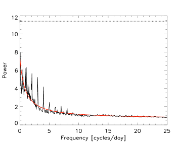
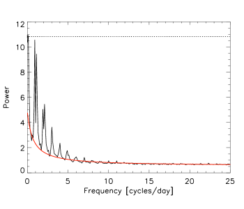
Figure 3.— Average Lomb-Scargle periodogram for the ensemble of 2007 (top) and 2008 (bottom) data. Dashed lines show the analytically determined 99% detection limit, as estimated with the Lomb-Scargle formalism. Red curves indicate our fit to the noise as a function of frequency, disregarding the systematic peaks at integer values. The roughly constant noise floor continues out to the Nyqyist limit at $\sim$65 (2008) and $\sim$100 c d^-1 (2007).

5.1. Periodogram Analysis

As an initial test for periodic variability in the data, we produced Lomb-Scargle periodograms (Scargle 1982) for all light curves. False alarm probabilities (FAP) for detected peaks were determined from the prescription of Horne & Baliunas (1986), which is valid even for datasets with non-uniform time spacing. They estimated FAPs based on large simulations of data with added gaussian noise, and their result depends on the number of independent frequencies, which they denote $N_{i}$. The formula for the parameter $N_{i}$ is a function of the total number of data points and has been shown to significantly overestimate FAPs for small datasets (Reegen 2007). This issue is not of great concern to the current study, given the 300-500 points from each run. However, the test must still be used with caution, since it assumes all noise sources are white. In reality, the frequency-dependent red noise contributes significantly to the light curve RMS on $\sim$ 1-day and longer time scales. Consequently, FAPs can be severely underestimated at low frequency and somewhat overestimated at high frequency. The results of the Lomb-Scargle test are nevertheless suitable for eliminating targets with no detected variability from the sample. With a selection criterion of FAP$<$1%, we assembled an initial set of possible periodic variables for additional analysis.

The collection of Lomb-Scargle periodograms for all targets– variable or not– is also a useful tool for identifying systematic effects in the data that may cause certain frequencies to consistently appear at artificially high probability. This effect is often seen when color-airmass effects are not taken into account in the light curves, resulting in trends that mimic intra-night variability. Because of the very uniform sampling of our datasets, we expect most of these spurious frequencies to occur at or near multiples of 1 cycle per day (cd^-1). To quantitatively map out these values, we constructed a histogram from all frequencies corresponding to peaks significant at the 99% level in the Lomb-Scargle periodogram. This diagnostic plot confirms that there are indeed pile-ups near integer frequencies, and we discarded potential variability detections corresponding to periodogram peaks occurring only at these values.

As an additional way to identify suspicious frequencies and examine the typical variability power distribution in frequency-amplitude space, we also generated a mean periodogram from all $\sim$1500 objects in each field, as seen in Fig. 3. This plot clearly displays not only the mathematical clustering of “significant” peaks around integer frequencies but also the steep increase in the noise floor toward low frequencies. We attribute this latter effect to red noise and fit it with an exponential of form $P=a_{0}+a_{1}/(f+a_{2})$, where $P$ is power, $f$ is frequency, and $a_{0}$, $a_{1}$, and $a_{2}$ are constant fitting parameters such that power declines to match the white noise baseline at $\sim 15$cd^-1 (e.g., “$1/f$” noise; Press 1978). The model for this $1/f$ component was incorporated into our computation of detection limits ($\S$5.2).

After removing from consideration targets with either no detectable variability or periodogram peaks only near integer frequency values, we performed additional analysis on the remaining light curves. All exhibited one or more peaks at the 99% significance level in the periodogram. To further probe these signals, we employed the program Period04 (Lenz & Breger 2005), which computes a fourier transform (Deeming 1975) of the light curve and may also be applied to time series with gaps. Results are similar to the Lomb-Scargle periodogram, but the program oversamples frequencies by a factor of 20 and contains an extended analysis package to calculate phases, subtract out signals, and search for periodicities at lower levels. Our input light curves were shifted to zero mean and cleaned of outliers at more than 4 standard deviations. Period04 includes an option to assign weights to each data point, such that deviant points do not overly influence the determination of the periodogram. However, based on our assessment of light curve RMS as a function of magnitude we conclude that uncertainties are difficult to determine on a point-to-point basis. We believe the approach of neglecting weights but removing clear outliers is therefore sufficient to accurately identify the frequencies of variability in the sample.

For each light curve, we used Period04 to identify the largest peak in the periodogram and extract a preliminary amplitude and phase for each epoch of observation. We then used the program to perform a non-linear least-squares fit for frequency, amplitude, and phase. A corresponding sinusoid was then subtracted from the light curve (this procedure is known as “prewhitening”) and a new periodogram was produced. We examined the residuals to determine whether they contained further significant frequencies or were consistent noise. If another suspected peak appeared, the data were once again prewhitened and the original light curve subjected to a multiperiodic least-squares fit (Sperl 1998; Lenz & Breger 2005). We repeated the process until all significant fourier components were extracted from the data. While significant harmonics appeared in cases where periodic variability was not completely sinusoidal, in no case did we identify multiple unassociated periods in a single object.

The statistical significance of identified peaks is difficult to determine directly but can be estimated from the noise properties of the periodogram. One criterion for detection of a signal to better than 99.9% certainty proposed by (Breger et al. 1993) requires S/N$>$4 in the amplitude spectrum (see also Kuschnig et al. 1997). For individual periodograms, noise levels were computed from the prewhitened periodogram as a running mean over boxes of 10 cd^-1 in frequency. We confirmed that no peaks remained at more than four times the noise baseline. As an additional check that all significant periodic components were removed from the data, we examined the light curve residuals and compared them to the typical RMS of non-variable objects with similar magnitudes (as shown in Fig. 2). The values were generally consistent with the noise in the non-variable targets.

Errors for the derived frequencies and amplitudes can be computed analytically in terms of the average light curve noise and number of data points Breger et al. (1999), but this approach is known to underestimate the true uncertainties. The least-squares fit also provides an error matrix, but neither of these methods fully account for the properties of noise in the frequency domain. We have therefore opted to run a set of 500 Monte Carlo simulations with Period04 for each object displaying periodic variability. The detected signals are extracted, and remaining noise data points are randomly rearranged such that the original timestamps are preserved. The identification of periodogram peaks and least-squares fit to the light curve is then carried out as before for each simulated light curve. The distribution of frequencies and amplitudes returned by these simulations then determine our uncertainties. Since the distributions are not strictly gaussian, we estimate 1–$\sigma$ uncertainties based on the values enclosing 68% of the simulated data. For signals that are near the detection limit, the simulations take into account the possibility that noise causes an alias to be selected instead of the true peak. This effect is included in our uncertainties listed in Table 3, which are provided at the 3–$\sigma$ level.

5.2. Detection Limits

Knowledge of our sensitivity to light curve periodicities as a function of both amplitude and frequency is crucial to determining whether lack of variability in some objects is related to detection techniques or real physical properties. In the presence of pure white noise, the signal-to-noise ratio for detection of a periodic signal in a periodogram scales as $A\sqrt{N}$/(2$\sigma$), where $A$ is the amplitude, $N$ is the total number of data points, and $\sigma$ is the photometric uncertainty. Therefore, for long time series it is possible to detect signals with amplitudes well below the level of the uncertainties in light curves. For example, data from our 12-night CTIO observations in 2007 reach a noise level of 0.001 magnitudes in the periodogram for objects near $I$=17, making detections as low as $\sim$ 0.004 magnitudes (e.g., S/N=4) possible. Red noise diminishes our ability to distinguish signals below about 5-10 cd^-1, or periods longer than a few hours. But across most of the frequency spectrum, sensitivity to periodicities is nearly uniform since the time sampling for both runs was uninterrupted, apart from the consistent daily gaps. We find the mean periodogram to be entirely adequate in eliminating the anomalous peaks, and because of our relatively uniform sampling do not find any deviations other than multiples of one cycle per day.

Nevertheless, we must also determine the frequency dependence of our sensitivity to periodic signals, in the presence of red noise. We therefore measure the mean noise level at four characteristic frequencies (0.1, 1.2, 7.4, and 15.2 cd^-1; corresponding to periods of 10 days, 0.8 days, 3.2 hours, and 1.6 hours) at intervals of 0.5 magnitudes. The mean noise levels are determined by generating periodograms for all objects not displaying variability (as measured by an RMS within 1–$\sigma$ of the median for that magnitude). We then measure the power in the periodograms at each of the four frequencies, and average together the values in 0.5-magnitude bins. Since we expect to be able to detect periodic amplitudes at four times the noise level, we have plotted these results, multiplied by a factor of 4.0, in Fig. 4. These values represent the minimum amplitude detectable in a periodic variable, as a function of period and magnitude.

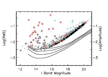
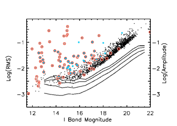
Figure 4.— Relative to the left axis, spread in photometry as a function of magnitude (top: 2007 data; bottom: 2008 data). Detected periodic variables are marked as blue dots, while confirmed and likely cluster members appear as red circles. Relative to the right axis, we plot the 99% sensitivity amplitude limit to periodic variability on four different time scales. From the top curve to bottom, these correspond to periods of 10 days, 0.8 days, 3.2 hours, and 1.6 hours. The 2007 field contains 1493 data points, while that from 2008 has 1683. Fewer objects appear at the bright end in the 2007 field because of variations in the underlying distribution of stellar magnitudes and also slightly different saturation limit.

In some cases, objects displayed signs of variability that were too weak to confirm. Those with unexpectedly high residual RMS but no obvious periodogram peaks were set aside for further analysis as part of the aperiodic variability group (§6). For targets with a possible peak in the periodogram just below the S/N$>$4 criterion, we analyzed the light curves produced by both image subtraction and standard aperture photometry; because of the slightly different processing, occasionally a low-level signal appeared with one method but not the others. For the particularly faint BDs with photometry was subject to large sky background noise, we required the peak to pass several tests for detection. First, when the putative signal is subtracted from the light curve, any other high-amplitude structure in its immediate vicinity (e.g, within $\sim 5$ cd^-1) must also disappear. Peaks that prove difficult to remove cleanly are typical of noise. Furthermore, we look for signals with one distinct peak, as opposed to two or more of roughly equal height separated by $\sim$1 cd^-1. Multiple peaks this close are not probable given the types of variability expected in VLMSs and BDs (e.g., one peak corresponding to the rotation period, and one or more additional peaks due to rotation of a binary companion or pulsation, for which overtones should be separated by at least 5 cd^-1).

The final sample of periodic variables contains 84 objects with clear variability by all criteria. Phased light curves for these targets are presented in Fig. 5, and their measured properties are listed in Table 3. The majority are VLMSs with roughly sinusoidal variability. However, the shapes of 19 are more characteristic of traditional pulsators or eclipsing binaries, and their blue colors are indicative of locations in the background field. For completeness, these are included in Table 3 as well. We have also identified a small number of objects with possible but questionable periodic variability. In these cases, the RMS of the residual light curves remains significantly larger than the expected noise level after subtraction of the detected signal. Objects in this small sample may consist of either undulating noise levels or other sources of non-periodic variability and are noted as unknown variable type in Table 3.

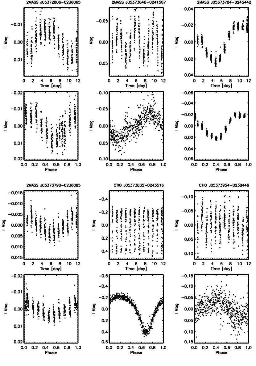
Figure 5.— Differential light curves with detected periodic variability, in order of right ascension. First and third rows show the original light curve, while those in the second and fourth rows are phased to the detected period. There are also a few that are not likely cluster members; membership status is listed in Table 3. Only the first panel of the figure is depicted here; Fig. 5 in its entirety is available in the online version of the Journal as well as %****␣sigori14_2column.tex␣Line␣725␣****www.astro.caltech.edu/~amc/SigmaOri.html.

6. Aperiodic variability detection

Past monitoring campaigns have revealed not only well-behaved periodic variability among low-mass young cluster members, but also sporadic, aperiodic brightness fluctuations likely indicative of accretion or time-variable disk extinction. While the light curves are a challenge to analyze quantitatively, their features offer clues into the mechanisms behind star-disk interaction. To fully mine our data for variables of all types, we have subjected the light curves to a battery of statistical tests in addition to the periodogram analysis. We examine the RMS magnitude spread for light curves of all objects in each of the two observed fields, as shown in Fig. 4. Such plots are standard tools for not only assessing the photometric performance, but also identifying outliers whose light curve RMS greatly exceeds the expected precision and hence suggests underlying variability. While the overall spread in light curves is well modeled by a combination of poisson errors, sky background, and a small systematic uncertainty ($\sim$0.002 magnitudes), many outliers that were not identified through the periodogram analysis are obvious in Fig. 4– indicating variability of a more erratic sort.

6.1. Chi-squared analysis

To distinguish between true variables and photometric errors, we disregarded targets with photometry clearly affected by bad pixels, saturation, or close proximity to neighboring stars, as the large RMS values are due to measurement issues rather than intrinsic variability. We subjected the remaining group of objects with inexplicably large RMS to a reduced Chi-squared criterion: if the photometric uncertainty of an individual data point $x_{i}$ is $\sigma_{i}$, then for a light curve with mean 0 and N total points, we have:

$$\chi^{2}=\Sigma\frac{x_{i}^{2}}{\sigma_{i}^{2}(N-1)}.$$

In addition, the measured standard deviation of the light curve, $\sigma$, is given by:

$$\sigma^{2}=\Sigma\frac{x_{i}^{2}}{(N-1)}.$$

If the individual photometric uncertainties are well represented by some typical value dependent on the object magnitude $m$, e.g., $\sigma_{i}\sim\sigma_{\rm typ}(m)$, then we see that the reduced $\chi^{2}$ criterion translates to a requirement on the standard deviation:

$$\chi^{2}=\frac{\sigma^{2}}{\sigma_{\rm typ}(m)^{2}}.$$

To detect aperiodic variables with an estimated 99% certainty, we select only light curves with $\chi^{2}>6.6$, or equivalently, a spread of more than 2.58 times the photometric uncertainty. These values are approximate, since the noise is not strictly gaussian, as assumed by the statistics. We estimated typical photometric uncertainties by performing a median fit as follows to the RMS as a function of magnitude using the combined poisson, sky, and systematic noise model: The values of all three noise sources were fixed (as a function of magnitude) according to the noise model components derived in $\S$4.2. A constant was then added to the model and adjusted such that half of the RMS light curve values lay above the model, and half lay below. The detected periodic variables as well as all 3-$\sigma$ outliers were rejected, and the fitting process was iterated until the median-fit function did not change. The variability detection cut-off was then taken to be the median fit, raised by a factor of 2.58. These curves are superimposed on the data in Fig. 6.

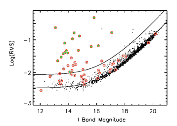
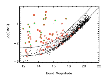
Figure 6.— Same as Figure 4, except now showing aperiodic variables in green. We plot the estimated total contributions from poisson, sky, and systematic noise, shifted upward by 0.12 dex so as to match the median of the data (solid line). The curve corresponding to 99% probability of variability detection via the $\chi^{2}$ test appears above this.

Like the periodic variability search, the excess RMS analysis was conducted on all objects with available photometry, irrespective of cluster membership status. After selection of probable variables via the $\chi^{2}$ criterion, we overplotted in Fig. 6 those confirmed or likely to be members. It is evident that the vast majority of high-amplitude variables in our fields are known $\sigma$ Ori members, and the remainder are therefore good candidates. Objects exhibiting large RMS light curve spreads but not shown as variables (green dots) in Fig. 6 were already found to be periodic (e.g., $\S$5) and displayed instead in Fig. 4. Quite a few of the identified periodic variables lie below the $\chi^{2}$ detection threshold, indicating the power of the periodogram for identification of variability isolated to specific frequencies. In addition to the $\chi^{2}$ test, we probed all light curves for variability by calculating the single-band Stetson index (e.g., Stetson 1996), which is a measure of the degree of correlation between successive data points. The distribution of Stetson index as a function of magnitude was fairly tight, such that the number of variables selected was relatively insensitive to the threshold chosen for variability detection. While this test confirmed all cases of aperiodic variability uncovered with the $\chi^{2}$ criterion and a number of the previously identified periodic variables, it did not reveal any additional variable objects. This result may reflect a large typical intrinsic light curve scatter for the aperiodic variables in our sample.

In total, we identified 42 aperiodic variables, as listed in Table 4 and shown in Fig. 7. In order to explore the relationship between erratic variability and the presence of disks and accretion, we have noted the objects in Table 1 with observed infrared or near-infrared excess, and also provide the H$\alpha$ equivalent width where available in Table 4; in $\S$7.4 we discuss the correspondence between these quantities.

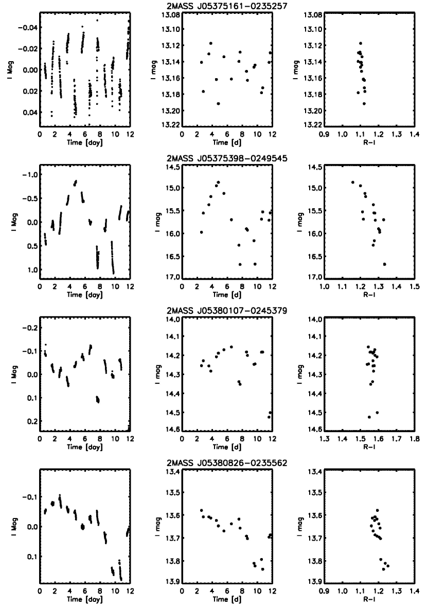
Figure 7.— Light curves selected as aperiodic based on large $\chi^{2}$ values and lack of periodicities. Objects are arranged in order of right ascension, and membership information is available in Table 4. The left column displays the full $I$-band light curves, while the middle shows the same data at the reduced cadence corresponding to the $R$-band observations. The right column shows $R$-$I$ color trends. Figure 5 in its entirety is available in the online version of the Journal as well as www.astro.caltech.edu/~amc/SigmaOri.html.

6.2. Sensitivity to combined aperiodic and periodic variability

In $\S$5.2 we simulated our sensitivity to photometric periodicities at different frequencies by assuming that the underlying light curves are well represented by a combination of simple noise sources (white and red) and a single sinusoidal signal. However, the large number of aperiodic variables detected via the $\chi^{2}$ test indicates that many light curves are in fact dominated by other types of variability, such as that associated with accretion. In these cases, we may not be able to detect periodicities superimposed on the larger-amplitude erratic fluctuations. We have investigated this reduction in sensitivity by injecting sinusoids of various frequency and amplitude into the light curves of a large subset of our aperiodic variables. The sample includes objects with RMS ranging from 0.01 to 0.3 magnitudes and $I$-band brightnesses from 12.0 to 17.5 magnitudes. We then attempted to recover the injected signals in the periodograms. The erratic nature of these light curves produces a steep trend in the frequency domain similar to the red noise from correlated photometric errors, but reaching higher amplitudes.

Since detection of periodic variability is frequency dependent, we have performed signal recovery tests in three regimes: frequencies less than 1 cd^-1 (e.g., periods greater than 1 day), frequencies between 1 and 3 cd^-1, and frequencies greater than 3 cd^-1. These domains were chosen based on the typical exponential shape that we find for periodograms in our aperiodic variable sample. Our tests indicate that the periodogram noise levels for these objects are well correlated with the RMS spread in their light curves, regardless of brightness. This RMS ranges from 0.01 to 0.4 (see Table 3) and should not be confused with the photometric noise level, which is typically much smaller. Amplitudes of the injected signals ranged from 25–400% of the RMS for the two lower frequency regimes and 5–50% of the RMS for the high frequency regime.

Most of the injected signals appeared clearly in the periodogram, but the decision as to whether they were “detectable” depended on the surrounding noise level. For frequencies less than 1 cd^-1, the mean periodogram noise is approximately the light curve RMS divided by 2.2 (e.g., $\sim$0.45$\times$RMS), whereas for frequencies from 1 to 3 cd^-1, this decreases to the RMS divided by 2.9 (e.g., $\sim$0.34$\times$RMS). Noise in the periodograms of aperiodic variables decreases drastically toward higher frequencies or short periods, and consequently for frequencies beyond 3 cd^-1, the mean periodogram noise level decreases to RMS/23 (e.g., $\sim$0.04$\times$RMS). Detectability of a periodic signal requires an amplitude of at least 4.0 times the periodogram noise level. Therefore, our ability to detect periodic signals superimposed on aperiodic variability requires periodic amplitudes larger than $\sim$1.8$\times$RMS, $\sim$1.36$\times$RMS, and $\sim$0.16$\times$RMS in the three respective frequency ranges. Based on a median periodic variability amplitude of 0.02 magnitudes, we then expect to detect both aperiodic and periodic variability in cases where the period is less than eight hours (e.g., frequency $>$3 cd^-1) and the RMS of aperiodic variability is less than 0.13 magnitudes. It may also be possible to detect periodicities with longer periods, but only if the RMS of aperiodic variability is near 0.01– an uncommon occurrence, according to Table 3. We conclude that it is a challenge to identify both periodic and aperiodic variability in individual objects because of the different characteristic amplitudes of these phenomena.

7. Variability in the Context of Stellar and Circumstellar Properties

We have identified 126 variables in our fields, including at least 107 suspected $\sigma$ Ori members (101 of these are previously proposed members and six are candidate members newly identified here). In Fig. 8 we present $R$-$I$ versus $I$ optical color-magnitude diagrams derived from our photometric data (§4.3) and overplotted with 3 Myr theoretical isochrones from Baraffe et al. (1998) and D’Antona & Mazzitelli (1997), incorporating a conversion to photospheric colors using color-temperature and bolometric-correction-temperature relationships, along with a distance of 440 pc (Sherry et al. 2008). The vast majority of the variables fall above the main sequence and along a possible young cluster sequence. This finding confirms that single-band photometric monitoring is an efficient way to identify pre-main-sequence low-mass stars and brown dwarfs, and thus an effective technique in fields where the pre-main-sequence stars do not stand out in color-magnitude diagrams as distinct from the field stars.

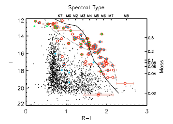
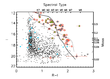
Figure 8.— $R$ and $I$ color-magnitude diagrams for all objects with photometry (black dots) derived from our fields (top: 2008; bottom: 2007). Red circles are confirmed and candidate $\sigma$ Ori cluster members, while cyan filled circles are detected periodic variables and green filled circles are aperiodic variables. We have overplotted 3-Myr isochrones from Baraffe et al. (1998) (solid curve) and D’Antona & Mazzitelli (1997) (dotted curve) to illustrate the theoretically predicted sequence for young cluster members. Masses are from Baraffe et al. (1998), but those from D’Antona & Mazzitelli (1997) are similar. Spectral types shown were derived from the empirical relationship between $R$-$I$ and spectral type among objects in our data and a few from $\sigma$ Ori datasets in the literature. The two fields exhibit different average reddening due to spatial variations in extinction.

The light curves and their temporal properties offer insights into the origin and prevalence of brightness variations, which we discuss in $\S$7.1. Yet we can also make use of the rich array of data from previous spectroscopic studies (e.g., Table 1) as well as the $Spitzer$ mission to analyze variability from several additional angles. In the forthcoming sections, we assess the correlations of variability with stellar and circumstellar properties. The $R$-$I$ photometry available from our work provides not only information on the relationship between brightness and color changes ($\S$7.5), but also a means to investigate the mass-dependent properties of young stars and brown dwarfs ($\S$7.3). In addition, we employ mid-infrared data to connect variability with the presence of disks around these objects ($\S$7.4).

7.1. Overall variability properties

7.1.1 Variability classification and persistence

Characterization of variability can illuminate our understanding of the physical processes that take place on and around few Myr old low-mass stars. We have identified several types of variability among our sample of 126 variables, including irregular variability and various forms of periodic variability such as spot modulated stellar rotation, pulsations, and full or partial eclipse signatures, as listed in Table 3. Among 147 previously known or suspected cluster members included in our photometry, the overall variability fraction is 69%, with irregulars (27%) and periodic objects (42%) comprising this cluster sample. Furthermore, we uncovered 25 variables with no prior membership information, most of whose light curves resemble eclipsing binaries or short-period pulsators. However, six have colors consistent with membership in $\sigma$ Ori and light curves consistent with either spot modulation or accretion. Since these six objects encompass a range of brightnesses, it is not clear as to why they they were missed in previous surveys. The new candidates are included in Table 1 and noted in Tables 3 and 4 as possible members. Just under half (44%) of objects in the remaining 31% of our sample for which no variability is detected have strong evidence for $\sigma$ Ori membership based on Table 1. Hence we conclude that at least 15% of young cluster members may not display obvious brightness fluctuations on time scales up to two weeks.

Among the 41 $\sigma$ Ori members in our fields previously identified as variable objects (35 aperiodic and 6 periodic; see Appendix A), we confirm variability in 33 (30 aperiodic and 3 periodic); this suggests that the variability mechanisms are long-term rather than sporadic phenomena. In the subset for which we do not redetect variability, there are no particular biases toward long or short time scale. We suspect that the combination of low numbers of data points, uneven time sampling, and underestimated uncertainties could have contributed to previous false detections in some cases. However, it is also possible that the variability mechanism itself turned off during the time of our observations.

In addition to comparing our variability detections with those of other works, we can use our own repeat observations of the 2007 field to glean further information about the time scales on which various types of variability operate. While the small number of data points per light curve (23, or two per night taken in 2008) precludes detailed comparison of variability properties from one year to the next, we can nevertheless identify objects with high-amplitude variability persisting on this longer time scale. Of the 17 aperiodic variables found in our 2007 field, we re-detect all of them again in 2008, based on the $\chi^{2}$ analysis described in $\S$6.1. In addition, 22, or over 80%, of our 27 periodic variables identified as likely $\sigma$ Ori members in the 2007 field display significant variability at a similar period (the majority agreed to within 5%) in 2008.

We can estimate a minimum characteristic timescale, $T$, on which the various types of variability operate by considering the set of all objects with repeat observations separated by at least one year. In total, there are 52 aperiodic variables that were either observed in both 2007 and 2008 by us, or identified by another group and observed later by us. Of these, 47 displayed aperiodic variability during both sets of observations. We suppose that for a typical duration of accretion (or other source of aperiodic variability) $T$, the probability that variability will persist one year after its initial detection is $p\sim e^{-1/T}$. Taking this probability to equal 47/52, we find the typical characteristic for aperiodic variability time scale to be $T\sim 10$ years. A similar result is obtained using a binomial distribution to describe the probabilities for the outcomes of measuring variability.

Likewise, we can perform the same analysis for the periodic variables. In this case, 25 of 33 objects exhibited variability at roughly the same period during repeat observations over one year apart. The corresponding time scale for persistence of periodic variability is then at least $\sim$4 years. Based on these results, we conclude that the types of variability present among these young cluster sources are long-lived in comparison to the objects’ rotation periods ($\sim$1–10 days) as well as the intra-night time scale of abrupt light variations seen in aperiodic objects.

7.1.2 Variability demographics across time scale and brightness

In addition to visual classification of light curves, we can also consider variability properties in the time and magnitude domains. In doing so, it is important to understand any selection or other effects that may mask certain kinds of variability from being observed. The observing set-up imposes practical constraints on variability detection through photometric cadence, precision, interruptions, and total duration. These details translate into a maximum detectable amplitude for periodic variables and sets the range of detectable periods. The demographics of variability present additional considerations for our ability to classify light curve behavior. Some fraction of young stars and brown dwarfs may not have magnetic spots, or their surface features may be too small to induce observable variability and potentially infer a rotation period. Other objects may have multiple sources of variability (e.g., spots, accretion, circumstellar variability) that are difficult to separate from each other. In what follows, we carefully consider the connection between these effects and the variability trends that we have uncovered.

In the time domain, our observations are sensitive to photometric periods between $\sim$20 minutes and $\sim$12 days, as discussed in $\S$5. While we do encounter periodic variability close to the longest possible time scales, we detect no periodicities on the shortest time scales– less than 7 hours (e.g., Fig. 9). If this effect is the result of our photometric sensitivity, then it should be explained by the detection limits determined in ($\S$5 and §6). Instead, we find (Fig. 4) that we are more sensitive to short periods and could recover signals down to 0.001 magnitude amplitudes for objects brighter than $I$=16, or signals with 0.01 magnitude amplitudes out to $I\sim$19 or 20. Another possibility is that we are somehow missing periodic variability in cases where the light curves are dominated by aperiodic behavior. In $\S$6.2 we concluded that we are likely to identify both types of variability in a single object only if the time scale for the periodic component is less than 8 hours and the light curve RMS is below $\sim$0.13 magnitudes. A number of the detected aperiodic variables do indeed have RMS values that satisfy this criterion (Table 4). Hence while detection limits may explain our failure to identify combinations of aperiodic variability and longer time scale periodicity in single targets, they do not account for the dearth of short-period variables. We conclude that the lack of periodic variability on time scales under 7 hours is a real physical effect.

Changes in variability properties as a function of magnitude can also shed light on the properties of young stars and brown dwarfs. To estimate the correspondence between mass, $I$-band magnitude, and $R$-$I$ color, we have overlaid 3 Myr theoretical isochrones from Baraffe et al. (1998) and D’Antona & Mazzitelli (1997) on our data in Fig. 8. Since reddening is low in $\sigma$ Ori, the observed $R$-$I$ values are close to the intrinsic photospheric colors. Although mass predictions are fairly uncertain at these ages (Baraffe et al. 2002), the two models agree well with each other and we have adopted the mass values of Baraffe et al. (1998). These estimates indicate that our dataset encompasses objects with masses from approximately 0.02 to 1.0 $M_{\odot}$. The substellar limit, at $\sim$0.08 $M_{\odot}$, lies near $I$=17 or spectral type M6. The spectral types shown in Fig. 8 were adopted directly from the objects in our $\sigma$ Orionis sample with available spectroscopy (Table 1).

We find variables of all types spanning the entire range of magnitudes, but Fig. 8 displays a subtle decrease in variable cluster members at the faint end, which might be explained by the decline in photometric sensitivity. For the subclass of variables identified as aperiodic, we note that the brightest objects have light curve RMS values from 0.03 to 0.2. Based on the detection limits described in $\S$6, we lose sensitivity to this type of variability around an $I$ magnitude of 18.0. For objects brighter than this limit, we find that aperiodic variables seem to populate the entire range of magnitudes, including a portion of the brown dwarf regime. Attributing aperiodic variability to accretion and its associated hot spots or fluctuating dust extinction levels, we do not find significant evidence for physical changes in these effects across the substellar boundary.

Magnitude trends in periodic objects are slightly more difficult to determine, as they are dependent on period as well as the potential presence of aperiodic variability at larger amplitude. Our detection limits (Fig. 4) indicate that we are sensitive to amplitudes of $\sim$0.01 magnitudes out to $I\sim$18.5-19.5, depending on period. Thus we should be able to detect whether the properties of periodic variability are similar from the stellar through the brown dwarf regime. If we divide our sample into “bright” ($I<17$) and “faint” ($I>17$) groups, we find the fraction of periodically variable faint objects to be 34$\pm$10%. Compared to the number of targets that are periodically variable at brighter magnitudes (46$\pm$6%), there appears to be a reduction in the fraction of variable members for faint magnitudes and thus lower mass. The significance level of this finding is difficult to assess since cluster membership status is not secure for many of the fainter objects. However, if we restrict our estimate to confirmed (e.g., via spectroscopy or infrared excess) cluster members, the periodic variability fractions are similar to those of uncertain cluster members: 45$\pm$7% for objects with $I<17$, and 26$\pm$12% for those with $I>17$. The majority of periodically variable cluster members display roughly sinusoidal light curves consistent with rotational modulation of stellar spots. Therefore the apparent reduction in periodic variables toward fainter magnitudes suggests a difference in the photospheric properties of young brown dwarfs, as compared to the higher mass stars.

7.2. Origin of periodic variability

The periodic variability in our cluster sample is most likely due to spot modulation of the light curves. On time scales of 0.3–12 days and with amplitudes of 0.003–0.12 mag, the periods of the brightness changes among known and suspected cluster members are too long to be explained by the pulsation theory (Palla & Baraffe 2005). We would have detected the shorter periods predicted by the theory if they had amplitudes of $\sim$0.001 (bright sample; $I<$16) to 0.01 magnitudes (faint sample; $I\sim$20). Further, the roughly sinusoidal shapes of the periodic variables are not consistent with other varieties of pulsators or a population of eclipsing systems, apart from the 19 field objects listed in Table 3. Instead, the time scales and amplitudes are compatible with modulation of spots that may be either cooler than the photosphere, as in active chromosphere models, or hotter than the photosphere, as in accretion column models (Carpenter et al. 2001; Scholz et al. 2009). Comparison of theoretical spot models with multi-color photometric data has shown that both scenarios can produce larger amplitude light curves at shorter wavelength (e.g., Frasca et al. 2009). Although we have a small sample of $R$-band data points for each target, the color data are not extensive enough to allow for detailed modeling. In either case we assume that the periodicities extracted from our analysis can be attributed to rotational modulation of surface inhomogeneities and directly adopted as rotation periods.

7.3. Rotation rates in $\sigma$ Orionis

7.3.1 Distribution with color/mass

For “higher” mass ($>$0.3–0.4 $M_{\odot}$) stars in the ONC, NGC 2264, and IC 348 clusters derived periods have in some cases revealed double-peaked distributions, with two groups clustered near 1-2 and 8-10 days (Herbst et al. 2002; Lamm et al. 2005; Cieza & Baliber 2006). For other young cluster datasets, the distribution is not bimodal but peaks near 3–5 days (Cieza & Baliber 2007; Irwin et al. 2008). In contrast, our $\sigma$ Ori sample extends well into the brown dwarf regime and the corresponding periods cluster at short time scales, 1-2 days, with a uniform or exponentially decreasing tail extending out to and perhaps beyond 10 days. Only a few objects in the sample have periods in the 8-10 day range. Since the dataset includes a representative sampling of the $\sigma$ Ori IMF between $\sim$0.02 and 1.0 $M_{\odot}$ it is possible to search for trends in the period distribution along the color and magnitude axes.

In Figs. 9 and 10, we present the period as a function of $R$-$I$ and $I$, both of which serve as a proxy for mass since extinction is low. Included are only those periodically variable objects with solid or likely cluster membership status based on colors and spectroscopic data available in the literature (Tables 1 and 3). In this way, contamination by periodicities of field variables should be negligible. Apart from one or two outliers, there is a significant decrease in period with progressively redder color or fainter magnitude, implying that within this mass range, lower mass objects rotate faster than the higher mass ones. Taking the substellar boundary to be near spectral type M6 or $R$-$I\sim 1.9$ and $I\sim 16.5$ (see Fig. 8), there are nine brown dwarfs in the rotation sample with periods ranging from $\sim$7 hours to $\sim$3 days. On the other hand, the higher mass stars with $R$-$I<1.3$ or $I<14.3$ and $M\gtrsim 0.45M_{\odot}$ have periods larger than 4.5 days, with the exception of one object. The correlation of period with mass is statistically significant at the $10^{-6}$–10^-5 level, depending on whether the test is run on period and color or period and magnitude. Masses estimated from photometry are dependent on the theoretical model used, and the values presented here are derived from Baraffe et al. (1998), based on $I$-band magnitude and an age of 3 Myr. Previous works have used cut-offs between young “low” and “high” mass stars of spectral type M2.5 and masses of either 0.25 or 0.4 $M_{\odot}$ depending on the theoretical model (e.g., Herbst et al. 2007). We adopt a slightly higher value of 0.45 $M_{\odot}$ corresponding to $I$=14.3 and find that 78% of our sample falls in the low-mass end.

Figure 9.— Period of variables versus their $R-I$ color. Variables without obvious periods are not included, nor are those periodic variables having colors inconsistent with cluster membership. Objects with infrared excesses indicative of disks ($\S$7.4) are marked as open circles, whereas objects without evidence of a disk are filled circles. In the top diagram, we have overplotted models of constant specific angular momentum ($j$) derived from radii provided by the 3 Myr isochrones of Baraffe et al. (1998) (solid curve) and D’Antona & Mazzitelli (1997) (dotted). The dotted line at the right side represents the completion limit redward of which we cannot detect periodic signals of amplitude less than 0.007 magnitudes. In the bottom diagram, we overplot models of constant angular velocity from the same isochrones. In both plots, we show estimated break-up periods derived from mass and radii predicted by the same theoretical models.

Figure 10.— Period of variables versus their $I$-band magnitude. The sample, as well as the symbols and curves, are the same as in Fig. 9. Likewise in the bottom diagram, we show models of constant angular velocity.

An intriguing aspect of our data is that several regions of the color-period and magnitude-period diagrams are nearly devoid of data points. Only one cluster member appears with a rotation period less 14 hours. This finding cannot be a result of our detection limits, as our sensitivity increases on shorter time scales ($\S$5.2). To test whether a short-period cut-off might be explained by the maximum allowed rotational velocities, we have estimated the periods required for break-up as a function of mass, using masses and radii from the 3 Myr models of Baraffe et al. (1998) and D’Antona & Mazzitelli (1997). Break-up is assumed to occur when the centrifugal force from rotation exceeds self gravity; the results of these computations are shown in Figs. 9 and 10. The break-up periods increase slowly with mass and range from 2 to 7 hours, and thus there is a significant gap between the break-up curve and the observed rotation data. Consequently, some physical mechanism seems to limit the rotation speed of most low-mass objects to at most 40% of break-up, and even slower speeds at higher mass.

In addition to a lack of variability on few-hour time scales, we also find a dearth of periodic variables in two other regions of the period-color and period-magnitude diagrams: from Figs. 9 and 10, we see that only two blue objects (e.g., $R$-$I\lesssim$1.3, $I\lesssim$14.3, or spectral type earlier than M2.5) rotate with periods faster than 3 days, and only one of the redder objects (e.g., $R$-$I>1.5$, $I\gtrsim$15, or spectral types later than M3.5) rotates with a period greater than 3.2 days. It is these two largely empty regions that conspire to create the pattern of increasing period with mass. To confirm that this trend is not a data selection effect, we have explored several scenarios that might prevent detection of rotation periods in the two regions.

As emphasized previously, our sensitivity to periodic signals increases on shorter time scales down to 20 minutes; hence this does not explain the gap in period detections at the bright end. However, detection also depends on variability amplitude. In Fig. 4, we have shown that we are sensitive to amplitudes of $\gtrsim$0.001 magnitudes for the brightest ($I<$16) and bluest objects. The entire sample of periodic variables associated with rotation has a mean amplitude of 0.02 magnitudes, with a standard deviation of 0.013 magnitudes. Thus we expect only a small fraction of periodic variables to display amplitudes less than 0.007 magnitudes. To determine whether a population of “missing” blue objects with such low amplitudes could explain the deficit of data points in the lower left portion of the color-period diagram, we examined the periodograms of all cluster members with $R$-$I<$1.3 and no detected variability. In the majority of these objects, we are able to rule out the presence of periodicities with amplitudes greater than 0.007 magnitudes. For those members that display aperiodic variability, identification of underlying periodicities is nearly impossible (see $\S$6.2). However, we see no reason that the light curves of aperiodic objects would contain periodic variability with preferentially short period, unless there is some additional spin-up due to ongoing accretion. Thus we tentatively conclude that there is a real deficit of $\sigma$ Ori members blueward of $R$-$I$=1.3 and $I$=14.3 with periods less than 3 days.

The second empty region of the color-period diagram, where $R$-$I\gtrsim$1.5 or $I\gtrsim$15, displays an apparent boundary at periods over $\sim$4 days. It is tempting to identify this as a physical trend, but not immediately clear whether it could simply reflect our diminished sensitivity to longer periods at faint magnitudes. To find the locus of colors, magnitudes, and periods for which we could detect periodic variability amplitudes as low as 0.007 magnitudes, we averaged all periodograms of non-variable field objects in 0.5-magnitude bins. For each bin, we fit an exponential curve to the mean periodogram, as in Fig. 3. To detect a signal of amplitude 0.007, the noise level must be approximately 1/4 of this, or 0.0018 magnitudes. The point at which the exponential fit reaches this value was then taken to be the minimum frequency required for a detection. We then converted this frequency to period, and employed an empirical isochrone fit to Fig. 8 to translate the $I$-band magnitude of each bin to an $R$-$I$ value. The resulting set of data points from all magnitude bins forms a locus on the color-period diagram which declines steeply with color, as shown by the completeness limit line in Fig. 9. Redward of this relation, we cannot uncover signals of amplitude less than 0.007 magnitudes and thus the periodic sample may not be complete. The locus crosses our maximum detectable period, $\sim$12 days, at $R$-$I\sim$2.0 and reaches a period of 1 day between $R$-$I$=2.1 and 2.15. While several data points fall redward of this line (these detections had higher amplitudes), a large swath of the empty region still lies on the blue side and cannot be explained by the completeness limit. As with the other gap in the color-period and magnitude-period diagrams, a survey of the periodograms of non-variable objects shows no evidence of overlooked periodicities with amplitudes greater than 0.007 magnitudes. It is once again possible that we may be missing periods in objects that are accreting and display high-amplitude erratic variability or have very small surface spots, but we cannot explain why these effects would only occur for certain combinations of colors and periods. Consequently, the trend of increasing period with decreasing color seen in Figs. 9 and 10 appear to reflect a physical correlation between rotation and mass.

To explore whether the gaps found in our period-color and period-magnitude diagrams are a general feature of young star and brown dwarf rotation, we have compared our data to the period-mass distributions of the similar age clusters NGC 2264 ($\sim$2 Myr; Lamm et al. 2005; Irwin & Bouvier 2009) and NGC 2362 ($\sim$5 Myr; Irwin et al. 2008). We in fact find quite a few objects with periods from 1–3 days across all masses. Nevertheless, there does appear to be a relative deficit of fast rotators at higher mass, as well as slow rotators at lower mass, similar to $\sigma$ Orionis. To compare rotation data from the three clusters more quantitatively, we have plotted them together in Fig. 11. $I$-band magnitudes from each set have been transformed to masses using the models of Baraffe et al. (1998), as well as cluster distances and $I$-band extinctions. Although there are inherent uncertainties to the theoretical models at this age, the systematic errors should be similar for each cluster. Superimposed on the data in Fig. 11 are median fits to each set of periods and masses, which are remarkably similar for each of the three clusters, particularly for masses below 0.4 $M_{\odot}$. In addition, the rotation distributions in all three clusters appear to transition to longer periods above this mass (which is model dependent and corresponds roughly to $I\sim$14.5 for $\sigma$ Orionis. A Kolmogorov-Smirnov test reveals no significant differences between the three period distributions from the brown dwarf regime up to 0.5 $M_{\odot}$ where our own data peter out.

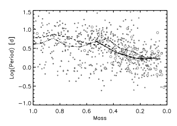
Figure 11.— Period of variables in our $\sigma$ Orionis sample (open circles), NGC 2264 (stars; Lamm et al. 2005), and NGC 2362 (small circles; Irwin et al. 2008) versus estimated mass based on $I$-band magnitude and the theoretical models of Baraffe et al. (1998). Curves show the the median period in 0.1 $M_{\odot}$ bins (or 0.15 $M_{\odot}$ for our sparser data): a dash-dotted line for Lamm et al. (2005), dashed line for Irwin et al. (2008), and a solid line for our own data, which stops at $\sim$0.55$M_{\odot}$.

7.3.2 Connection to internal structure and surface physics

The measured periods and amplitudes can inform us about the angular momentum and magnetic field properties of very low mass stars and brown dwarfs. The fact that rotation period seems to be connected with color or magnitude, and hence mass, implies that a physical conservation law may be at work.

Light curve period, $P$, is related to specific angular momentum, $j$, via $j\propto R^{2}/P$. If specific angular momentum from the natal cluster gas is conserved among $\sigma$ Ori members, then we expect periods to scale as $R^{2}$. The actual radii of our sample objects are unknown, but theoretical models predict their values with significant uncertainty due to lack of information about initial conditions, opacity, and treatment of convection (Baraffe et al. 2002). We have used the 3 Myr isochrones of Baraffe et al. (1998) and D’Antona & Mazzitelli (1997) to estimate $R^{2}$ as a function of mass. Converting masses to $R$-$I$ and $I$ as in Fig. 8, determination of a relationship between period and color requires the selection of a scaling constant to represent fixed specific angular momentum. Since the moments of inertia of young, low-mass objects are not well known, we have simply used one end of the observed color-period relation to anchor the calculated constant angular momentum function. We present the results in Figs. 9 and 10 (top panels) for data from both Baraffe et al. (1998) and D’Antona & Mazzitelli (1997); both curves fit the color-period data surprisingly well. In particular, the model derived from the Baraffe et al. (1998) isochrone can be adjusted so as to pass through the center of the data, reproducing the “gaps” seen in the lower left and upper right quadrants of the color-period diagram.

If young ($\sim$3–5 Myr) stars maintain constant angular velocity rather than angular momentum, we would expect periods to scale as $R$ instead of $R^{2}$. Although there is reason to believe that individual stars may evolve at constant angular momentum (Rebull et al. 2004, e.g.,), we have adopted this model primarily to illustrate how much freedom there is in fitting the data. We generated a constant angular velocity curve in the same way as we did for specific angular momentum and once again anchored one end to the observational data. As shown at the bottom of Figs. 9 and 10, this function fits the observed periods and colors almost as well as the $R^{2}$ model, although two curves derived from the D’Antona & Mazzitelli (1997) isochrone are a bit flatter than the data. So while there certainly seems to be a trend in periods with color and magnitude, it is not tight enough to conclusively determine its cause. In addition, a single outlier (2MASS J05391883-0230531) at $R$-$I$=0.7 and a clear period of 1.8 days confounds the idea.

While observed period may tell us something about physical properties of the variability mechanisms in the very-low-mass regime, light curve amplitude can also offer valuable information. This parameter is related to surface spot coverage and contrast. In Fig. 12, we show amplitude as a function of period for the sample of variables with good $\sigma$ Ori membership information. Short-period rotators appear slightly more likely to have amplitudes below 0.04 magnitudes than those with periods greater than 5 days, but it is difficult to sort out observational biases from this effect. Although different spot configurations may produce the same brightness patterns, we estimate a typical spot coverage of at least $\sim$2% based on the median 0.02-magnitude light curve amplitudes, assuming black spots. If, on the other hand, the temperature contrast between spots and the surrounding photosphere is closer to 80% (e.g., $T_{\rm spot}/T_{\rm phot}$), then coverage increases to $\sim$10%. Such contrasts and amplitudes are characteristic of either cool or hot spot covering fractions in young star samples (Frasca et al. 2009). Since amplitude does not appear to be correlated with period or color, we suggest that the mechanism producing the spots does not vary appreciably with rotation and possibly mass. Furthermore, because the majority of our objects are expected to be fully convective, the lack of correlation between spot coverage and other parameters may be indicative of uniform magnetic properties across the low-mass regime.

Figure 12.— Periods and amplitudes of variable $\sigma$ Orionis members. Most error bars are smaller than the size of the points.

7.4. The relationship between variability and circumstellar disks

Disks around young stars can be readily identified through thermal emission from circumstellar dust, manifest as infrared excess, or from gaseous emission lines attributed to accretion and outflow processes close to the star and seen spectroscopically. In this section we investigate the correlation between optical photometric variability and the evidence for circumstellar dust and gas.

We cross-referenced our photometric sample with that of Luhman et al. (2008), which provides $Spitzer$ Infrared Array Camera (IRAC; 3.6-8.0 $\mu$m) photometry derived from the observations of Hernández et al. (2007). We find that 133 of 153 confirmed or candidate $\sigma$ Ori members in our time series dataset have $Spitzer$ photometry, including 57 of 65 cluster periodic variables. IRAC photometry enables nearly unambiguous identification of unevolved disks in this cluster, as noted by Luhman et al. (2008). The $\sigma$ Orionis observations are unique among nearby young cluster observations with $Spitzer$ in that they were designed to search for disks around low-mass brown dwarfs and even planetary-mass objects; hence they are particularly deep. This gives us an unprecedented opportunity to study the relationship between variability, rotation, and presence of disks in the very low mass regime, potentially illuminating the reason why young cluster rotation period distributions have been reported to change around $\sim$0.25 or 0.4$M_{\odot}$ (Rebull et al. 2006; Cieza & Baliber 2007), and why the rotation periods in our own dataset appear to undergo a transition near $R$-$I$=1.3 ($\sim$0.45$M_{\odot}$; as discussed in $\S$7.3.1).

7.4.1 Disk selection criteria

We display in Fig. 13 the distribution of $Spitzer$/IRAC 3.6-8.0$\mu$m colors for all objects in our data with available infrared photometry. As seen in the figure, the sample splits relatively cleanly into two groups, with the narrower blue sequence near [3.6]-[8.0]=0 representing bare photosphere colors. The cloud of objects with [3.6]-[8.0] colors between 1 and 2 is indicative of infrared excesses signifying the presence of a dusty disk. While the sequence of photospheric colors is fairly well defined, several ambiguous objects lie between 0.3 and 0.7 magnitudes. We have therefore chosen a somewhat conservative disk selection criteria of [3.6]-[8.0]$>0.7$ (e.g., Cieza & Baliber 2007) so as to omit these objects from the disk sample. In total, we identify 47 likely $\sigma$ Ori members with both photometry from our campaign and Spitzer colors indicative of disks. The resulting disk fraction in our sample is roughly 35$\pm$5%. We find that our disk identification is entirely consistent with that of Hernández et al. (2007) and Caballero et al. (2007) (based on the same $Spitzer$ data), apart from one newly-identified disk-bearing object, 2MASS J05375398-0249545, which has a [3.6]-[8.0] color of 1.3. The full listing of disk classifications is provided in Table 1.

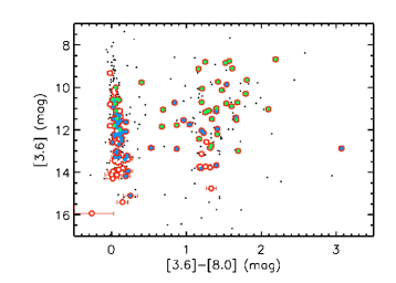
Figure 13.— Spitzer photometry of likely $\sigma$ Ori members (dots) from Luhman et al. (2008). Those found in our photometric sample are marked with red circles. Aperiodic variables detected in our photometry are overplotted as filled green circles, while periodic variables in our sample are marked by filled blue circles. The nearly vertical cluster of objects near [3.6]-[8.0]=0 is the sequence of colors and magnitudes pertaining to bare photospheres.

Previous works exploring connections between variability and the presence of disks often have relied on colors at shorter wavelengths to infer the presence of circumstellar dust. To test the suitability of this method, we produced another color-magnitude diagram using $R$-$J$ and $H$-$K$ colors, as seen in Fig. 14. Here the Spitzer-identified disk-bearing objects are highlighted by red squares. While there are a number of targets with sufficiently large $H$-$K$ to confirm a dust excess, many others that do have disks based on the $Spitzer$ data cannot be distinguished from the sequence of photospheric colors with $H$-$K$ ranging from 0.2 to 0.4.

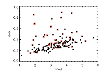
Figure 14.— $R$-$J$ and $H$-$K$ colors for $\sigma$ Ori cluster members in our sample. Disk identification at these wavelengths is possible for objects whose $H$-$K$ colors significantly exceed the trend in photospheric colors visible along thee bottom of the diagram. Targets for which Spitzer infrared data implies the presence of a disk are surrounded by red squares. Fewer than half of disk-bearing members would have been selected based on the near-infrared method.

7.4.2 Variability-disk connection

In Fig. 13 we have distinguished variable objects from the non-variables in the $Spitzer$/IRAC color-magnitude diagram. Not all of our photometric targets in $\sigma$ Ori are included in the $Spitzer$ sample due to varying spatial coverage. Of the 133 that are, we identified 97 as variables (e.g., Tables 3 and 4). The majority of objects with clear periodicities have no evidence for a disk (43 of 57), while a subset of 13 do show clear infrared excess. The disk fraction among period variables is thus $\sim$23$\pm$6%, somewhat lower than the overall disk fraction. However, this measurement may be biased by the fact that we cannot measure periods in disk-bearing objects that are undergoing relatively high amplitude accretion events. Four objects fall in the ambiguous category with [3.6]-[8.0] colors between 0.3 and 0.7. One of these (2MASS J05390808-0228447; [3.6]-[8.0]=0.53) has a clear periodicity with period 1.7 days and amplitude 0.02 magnitudes, similar to other variables that lack infrared excesses. The remaining three (2MASS J05390760-0232391, 2MASS J05390878-0231115, 2MASS J05392677-0242583) exhibit much more erratic and higher amplitude (RMS$\sim$0.2–0.3 magnitudes) variability.

In general, we can associate disks with the majority of aperiodic variables in our sample and lack of a disk with most of the periodic variables. This outcome is no surprise, since the aperiodic variability is likely due to accretion, which requires a disk. Likewise, since the variability in most of these disk-bearing objects is relatively high amplitude ($\sim$0.1 magnitudes RMS on average), we do not expect to detect many periodic variables among this sample, for the reasons outlined in $\S$6.2. But a number of objects do not fit these scenarios. Nine $\sigma$ Ori members display aperiodic variability but no sign of infrared excess in the $Spitzer$ data; the additional three objects highlighted above have only weak signs of an excess. On the other hand, 13 $\sigma$ Ori members with clear-cut infrared excesses display periodic variability with only low-level erratic behavior suggestive of accretion. In a few cases where signal-to-noise is particularly high (e.g., 2MASS J05391883-0230531 and 2MASS J05381866-0251388), it is possible to see that the phased light curve is a combination of a nearly perfect sinusoid and a small additional “blip” that may be ascribed to transitory accretion.

Since the $Spitzer$ data enables us to conclude only that an object is surrounded by warm dust, the association between an infrared excess and accretion (i.e., infall of gas), is imperfect. This may explain why a small fraction of objects identified as having disks do not exhibit aperiodic variability, if the gas supply in these systems has already diminished. Likewise, we conjecture that those targets displaying aperiodic variability but no infrared excess probably still have a gas component of a disk, whereas the dust is reduced or changed to the point of being undetectable at 8.0$\mu$m and shortward. In the following sections, we explore in more detail the connections between each type of variability and the presence or absence of a disk.

7.4.3 Relationship between disks and periodic variability due to rotation

The connection between stellar rotation period and disk presence has long been a subject of speculation. Disks have been invoked as a mechanism to remove angular momentum from young stars, in order to explain the slow rotation rates seen at older ages, as compared to models of spin-up associated with radial contraction (Bouvier 2007). But while some studies have claimed a correlation between rotation rate and disk presence (e.g., Rebull et al. 2006; Cieza & Baliber 2007), others have refuted the so-called disk-locking theory (Koenigl 1991; Makidon et al. 2004), particularly in the low-mass regime. To investigate the disk-rotation connection with our own data, we have examined the subset of 57 objects identified with both periodic variability and $Spitzer$ [3.6]-[8.0] data. Among these periodic variables, only 13 fall in the disk sample with infrared color excesses. Unfortunately for the majority of disk-bearing objects, we cannot photometrically measure most of their rotation rates because of the prominent high-amplitude aperiodic variability. But we can nevertheless plot the periodic sample against $Spitzer$ [3.6]-[8.0] color to discern any large differences between the rotation rates of objects with and without disks, as shown in Fig. 15. The sequence of likely diskless objects at [3.6]-[8.0]$\sim$0.0 contains a large spread of photometric periods from 8 hours to over 10 days. The objects with disks do have a slightly lower mean period, but this could be a selection effect. If there is a mass dependence for rotation or accretion properties, then this diagram may not indicate the true distribution of rotation periods. For example, if low-mass stars rotate faster but accrete for longer, then we may not be detecting a number of short rotation periods through the larger-amplitude fluctuations due to accretion in the light curves. In addition, the fraction of disk-bearing objects appears to increase from $\sim$40% of low-mass stars (0.1-0.5 $M_{\odot}$) to $\sim$60% of brown dwarfs in $\sigma$ Orionis (Luhman et al. 2008).

Figure 15.— $Spitzer$ [3.6]-[8.0] color versus rotation period for our periodic $\sigma$ Ori members.

To circumvent the possible mass biases from our data, we have highlighted the disk-bearing objects among the rotation sample in Figs. 9 and 10; these are indicated by open circles. The inclusion of color information in addition to periods and disk presence enables us to examine the effect of the mass distribution underlying our sample. We have seen from this diagram that the rotation periods have a marked and significant trend toward longer time scale at bluer color (and hence higher mass), as discussed in $\S$7.3.1. This correlation appears relatively independent of whether an object possesses a disk. To statistically test for differences between the rotation periods of objects with disks and without disks, we have plotted histograms of each distribution. We restrict both samples to $R$-$I>1.3$ since there are only two disk-bearing stars blueward of this boundary, and rotation rates of the diskless stars might be biased by mass. Using a two-sided Kolmogorov-Smirnov test (Press et al. 1992), we find that any differences between the rotation rate distributions of disk-bearing and diskless objects are not statistically significant, at the 7% level (i.e., $p$=0.93). Even if we expand the analysis to include stars with $R$-$I<1.3$, there remain no differences, at the 35% level $p$=0.65). With the caveat that the statistics are based on small numbers, we conclude that the disk-locking paradigm is largely inconsistent with our observations. The distribution of rotation periods instead appears to be set primarily by mass and additionally by a possible a third parameter.

7.4.4 Relationship between disks and aperiodic variability

In this section, we explore more directly a linkage between aperiodic variability, accretion, and disks. Erratic light curve variations in young stars have long been tied to spectroscopic signatures of accretion (Joy 1942), although they can have several origins (Herbst 1994). In particular, classical T Tauri stars, classified by their broad H$\alpha$ emission lines, undergo larger brightness fluctuations than the periodic variations more often seen in weak-lined stars Herbst (1994). The fact that most of our disk-bearing objects display variability that is both higher amplitude and more erratic supports this picture.

We can study the relationship between accretion and disk presence more directly by examining the available spectroscopy for our detected aperiodic variables. We have listed in Table 4 the H$\alpha$ pseudo-equivalent widths (pEW) where available from previous work. The value of this parameter is typically used to distinguish between H$\alpha$ emission that is chromospheric in nature, as compared to emission created in an accretion column and hence indicative of a disk. An equivalent width greater than 5–15 $\AA$ is typically chosen to identify accretors. We adopt here the criteria of Barrado y Navascués et al. (2003), in which the H$\alpha$ pEW boundary between accretors and chromospheric emitters varies with spectral type. The value varies from 7 to 11 $\AA$ across the M spectral type range typical of our sample. We find that 13 of our 17 aperiodic variables with H$\alpha$ pEW measurements from the literature have values consistent with accretion. The remaining four objects have fairly low RMS spread in their light curves that may indicate a different source for the variability.

Two of our targets with the largest H$\alpha$ pEW values are brown dwarfs, based on their faint $I$-band magnitudes: 2MASS J05382543-0242412 and 2MASS J05385542-0241208. The photometric data alone suggests that they are substellar accretors, because of the high-amplitude variability and lack of detectable periodicities. The former object was studied in detail by Caballero et al. (2006, ; see note in Appendix A), but the latter was heretofore unknown as a variable, although it was noted as having a broad H$\alpha$ emission line with an equivalent width of 190$\AA$ and other T Tauri-like spectroscopic features by Caballero et al. (2008).

To tie together the variability features, accretion indicators, and disk presence, we have compared the values of light curve RMS, H$\alpha$ pEW, and $Spitzer$ [3.6]-[8.0] color for our aperiodic variables. We detect no correlation between RMS and H$\alpha$ pEW, suggesting that the mechanism producing variability is somehow decorrelated with the strength of accretion. However, it must be noted that our photometry was taken well after (years, in many cases) the spectroscopic data. If either light curve amplitude or H$\alpha$ emission is highly time-variable, non-simultaneity of the observations may explain this finding. In addition, we have examined the relationship between these parameters and the infrared excess. Large H$\alpha$ pEW ($>10\AA$) compares well with infrared excess as a predictor of disk presence in that all but one target with values greater than $10\AA$ also have [3.6]-[8.0]$>$1.0. But once again, we do not see any noteworthy trends in RMS or H$\alpha$ with [3.6]-[8.0] color among targets identified as having disks.

There is a curious small population of objects, though, with RMS values ($\sim$0.01-0.03 magnitudes) much lower than the other aperiodic variables and whose H$\alpha$ pEW and [3.6]-[8.0] values suggest absence of accretion or an associated disk. In addition to having light curves in which variability is clearly obvious by eye, these objects have $\chi^{2}$ values high enough that their status as variables is not in doubt. All but one have $\chi^{2}>4.5$, or less than $10^{-5}$ probability that the light curve trends arose by chance; the remaining object (2MASS J05383922-0253084) has a $\chi^{2}$ value of 2.85, or an estimated 0.4% probability that its light curve behavior is explained by noise. We show in Fig. 16 the RMS and infrared color. The subset of nine low-RMS objects is seen as a cluster in the lower left corner and is clearly differentiated from the larger cloud of points with colors indicative of disks. Not all of these objects have available H$\alpha$ pEW values, but for those that do we find they are all low, between 0 and 10$\AA$.

Figure 16.— $Spitzer$ [3.6]-[8.0] color versus light curve RMS value for our aperiodic variables.

In summary, both H$\alpha$ emission and [3.6]-[8.0] color are good indicators of disk presence. Light Curve RMS is only a moderate indicator, since we encounter a number of disk-bearing objects with only low-level or periodic photometric variability. Of 47 targets identified with disks via $Spitzer$ data, we find 19 (40%) have aperiodic variability with RMS values above 0.05 magnitudes. The distinct advantage of photometric monitoring thus appears to be the ability to identify aperiodic variables for which the other indicators do not suggest a disk or accretion. The variability in these cases is difficult to reproduce without invoking some sort of circumstellar material, since its erratic and short-time-scale nature suggests a dynamic process as opposed to thermal or magnetic phenomena associated with the stellar surface. We suggest that this small population of objects does in fact have residual disks undetectable at $Spitzer$/IRAC wavelengths, with possible accretion or dust occultation as the source of low-level variability.

7.5. Peculiar variables

While over 40% of our detected variables are clearly periodic (Table 2; Fig. 5), some 27% are highly stochastic (Tables 3; Fig. 7). As discussed above, the former are associated with stellar rotation and the latter with processes associated with disk accretion. A number of intriguing objects among the stochastic class appear to have repeating patterns that are not, however, identified as periodic, the most prominent eight of which are shown in Fig. 17. They tend to display large-amplitude ($\sim$0.2-0.5 mag) dips of short duration (less than one day to a few days) in their light curves, preceded and followed by lower amplitude and longer time scale fluctuations. In some cases the fading can take up to a week. A few objects (2MASS J05382050-0234089 and 2MASS J05390276-0229558) display brightness dips with symmetric ingress and egress suggestive of some sort of occulting body; other brightness dips are rapid enough that we have only observed a portion of the event. Among all of the aperiodic $\sigma$ Ori light curves we identify approximately 20% of the sample that undergo fading events.

Stars displaying such distinct fading episodes may represent a low-mass analog of the UX Ori class (UXORs), in which brightness decreases of up to several magnitudes appear and persist for up to tens of days. The phenomenon has also been referred to as “Type III” pre-main-sequence variability (Herbst 1994). While it is typically associated with objects of spectral type K0 and earlier, it has been identified in the form of quasi-periodic, deep (i.e., on the order of a magnitude) brightness dips in a few T Tauri stars, notably AA Tau (Bouvier et al. 1999). Among the several theories that have been suggested to explain the prominent dips seen in these variables, the most common invokes extinction events, in which clumpy material in a surrounding disk occults the central object from time to time. As the opacity increases the star becomes fainter and redder until scattering dominates and the object becomes bluer as it continues to fade. Bertout (2000) accounted for the recurrence of brightness dips with a model in which the occulting region is a high latitude ”warp” that periodically obscures the star above the extinction of a flared disk that is typical over the rest of the orbit. For the more sporadic fading, another theory is that the behavior may be due to variable accretion (Herbst 1994).

Figure 17.— Aperiodic light curves with one or more unusually pronounced brightness dips.

The diversity of light curve properties for the “peculiar” variables discussed here hints at multiple origins for the fading events, some of which may be well described by the periodic disk occultation model. While all of these objects have been classified as aperiodic based on the lack of one or more discrete peaks in the periodogram, most do display signal patterns in the frequency domain that are not consistent with either white or red noise. These include five or more peaks or clusters of peaks in the periodogram, indicating semi-periodic light curve behavior. We find that two or three objects or $\sim$25-40% of this sample of eight as being quasi-periodic in their short duration fading behavior. This fraction is similar to the 28% estimated by Alencar et al. (2010) for periodic “AA Tau like” behavior in a comparable set of young stars in NGC 2264 determined from consideration of optical wavelength CoRoT data. Examining in detail the light curves of 2MASS J05390276-0229558 and 2MASS J05394318-0232433, we can estimate eclipse durations, depths and frequencies, assuming that the same “blob” of material is responsible for each fading event. For 2MASS J05390276-0229558, we estimate an eclipse repeat period of $\sim$1 day and duration of $\sim$0.2 day, while the light curve of 2MASS J05394318-0232433 displays dips of period $\sim$4 days and duration of $\sim$0.85 day. The stars, which are of similar $I$-band magnitude, have masses of $\sim$0.4 $M_{\odot}$ and radii $\sim$1.2 $R_{\odot}$, as estimated from the 3 Myr models of Baraffe et al. (1998). If the material is in a circular orbit, then its distance from the star can be deduced based on these stellar parameters along with the ratio of the eclipse duration to the repeat period. This rough estimate reveals that the occulting material must be extremely close to the star– within a stellar radius in both cases. In this scenario, the light curves may actually be displaying an impending accretion event, in which migrating material merges with the central star. If, on the other hand, the fading events are caused by distinct blobs of material, then their locations may be much farther out. The depths of the fading events ($\sim$4% and $\sim$15%, respectively) imply sizes for the material of 0.2–0.4 stellar radii.

The presence of disks around our peculiar variables also sheds light on the origin of brightness fluctuations. Based on Spitzer photometry ($\S$7.3) and the analysis of Hernández et al. (2007), we find that five of the eight peculiar variables shown in Fig. 17 are Class II type young stellar objects, surrounded by a thick disk but beyond the stage with significant high latitude (envelope) material. A further two objects (2MASS J05392677-0242583 and 2MASS J05390760-0232391) have weak $Spitzer$ infrared excesses ([3.6]-[8.0] color between 0.3 and 0.7). 2MASS J05392677-0242583 is probably an “anemic” disk (Lada et al. 2006), while 2MASS J05390760-0232391 was classified as a transition disk by Hernández et al. (2007) based on its large 24$\mu$m excess. The data suggest that both have optically thin inner regions. 2MASS J05390276-0229558, on the other hand, does not appear to have either a disk or any signs of strong H$\alpha$ emission. The fact that the intriguing eclipse-like variations seen in its light curve are much lower in amplitude than the other peculiar variables may indicate the presence of more consolidated disk material unobservable at $Spitzer$/IRAC wavelengths. For the majority of objects mentioned here, we believe the variability can be plausibly interpreted as extinction by “clouds” or geometric warps of relatively higher opacity than the disk atmosphere which produce fading events as the feature passes through our line of sight to the star while the disk rotates.

Color data can help further illuminate the source of peculiar variability, since we have not ruled out accretion effects. Different trends in color are expected depending on whether the variations are caused by extinction, disk scattering, or stellar spots, as explained by Carpenter et al. (2001) and Scholz et al. (2009). Since we have acquired $R$-band data twice per night for all targets, we can examine $R$-$I$ as a function of brightness for all aperiodic variables, and check whether any particular pattern stands out for the eight selected peculiar variables. We present in the right panel of Fig. 7 the available colors and magnitudes. Notably, with only lower cadence data (as represented in the middle panel) the richness and coherence of the light curve forms would be hidden. In many cases the fading events observed among our aperiodic variables are relatively colorless although both significant reddening and significant blueing is observed among the sample. We have measured the slope of reddening for all aperiodic variables in Fig. 7 by fitting a linear trend to the $I$-band magnitude as a function of $R$-$I$. We then negate the result so that slopes less than zero represent reddening as an object becomes fainter. The distribution of values is presented in Fig. 18. Although the color light curves do not have enough points to enable a detailed fit to the various variability models, we note that the vast majority of aperiodic variables show either negative or zero slope. For comparison, we have also plotted the value expected for pure interstellar extinction. Since the material in disks may be substantially different, we do not necessarily expect it to follow the same extinction law. Indeed, several of the peculiar variables display much more reddening during their fading episodes. The modeling by Carpenter et al. (2001) and Scholz et al. (2009) showed that hot spots from accretion can in fact exhibit steeper reddening slopes than extinction, at least in the near-infrared. This is certainly a possible explanation for some of our own sources. Only two objects in our sample, however, exhibit variability that may be accounted for by emission or scattering by the circumstellar disk, which is predicted to produce relatively blue fading events (Carpenter et al. 2001). Intriguingly, 2MASS J05390276-0229558, the only peculiar variable with no infrared excess, is one example. The single data point caught while this object was at its faint limit shows substantially bluer color than the rest of the light curve. We envision a scenario in which material temporarily occulting the star also scatters light toward us.

Figure 18.— Histogram of reddening values derived from the slopes of the $I$ versus $R$-$I$ trends displayed in Fig. 7. Negative values correspond to increased reddening with decreasing brightness. The dashed line marks the value for interstellar extinction, -E($R$-$I$)/$A_{I}$.

Although we cannot rule out the presence of accretion effects, we conclude that the hypothesis of occultation by disk material is qualitatively consistent with both the duration and the color-magnitude behavior of the brief fading events seen in the set of eight peculiar variables presented here. Further, as some of the events are periodic or semi-periodic, we note that the derived periods are consistent with those expected from an inner disk region in co-rotation with a star having typical spin for a Class II T Tauri star (2-10 days). Similar features located further out in the disk could be responsible for the non-repeating and/or broader fading events.

8. Discussion

We have presented photometric monitoring on a collection of low-mass stars and brown dwarfs in $\sigma$ Orionis. Extensive vetting of membership via prior spectroscopic information and the relative spatial compactness of our fields ($\sim$7 pc across) has ensured that the sample is relatively homogeneous in terms of age and initial conditions. In addition, the selection of $\sim$10-minute cadence and time baseline of nearly two weeks, along with excellent photometric precision has enabled us to carry out an unprecedented analysis of variability in young stars and brown dwarfs, complete to amplitudes below the 1% level for most sources. This combination of cadence and precision has allowed us to probe new areas of variability parameter space: those pertaining to short time scale and low-amplitude fluctuations. In the preceding analysis, we have explored the general properties of variability in very-low-mass $\sigma$ Orionis members and its connections to other stellar parameters. In putting the pieces together, we will now highlight the various phenomena encountered and possible connections to physical properties.

8.1. Variability in young stars and brown dwarfs is persistent - in time and mass

The sensitivity of our photometric monitoring has given us an unprecedented opportunity to probe for variability and explore its trends well into the brown dwarf regime. As discussed in $\S$7.1, we have detected variability of various forms in nearly 70% of our sample, including 85% of stars with strong evidence for cluster membership. The $\sim$15% of likely cluster members with no evidence for variability do not appear to have any distinguishing characteristics such as belonging to a particular mass range or possession of disks. This fraction is similar to the proportion of variables identified as periodic in 2007 but not in 2008. Using the 2007 field as well as data from other studies, we have also found ($\S$7.1.1) that the observed periodic and aperiodic variability is persistent on typical time scales of at least 5–10-years. This finding is consistent with studies of other clusters such as IC 348, in which analysis of data acquired by different groups retrieve largely the same photometric periods for objects in common (e.g., Cieza & Baliber 2006). Scholz & Eislöffel (2004) also carried out two photometry monitoring campaigns in another region of $\sigma$ Ori and identified a number of objects with persistent variablity across both datasets. Nevertheless they also suggest evidence for spot evolution based on a subset of targets displaying periodicities during only one campaign. While our analysis in $\S$7.1.1 points to long-lived accretion and magnetic activity on young, low-mass stars (in comparison to, e.g., the rotation period time scale), it is not sensitive to light curve amplitude or phase changes. Thus magnetic spots may come and go, but the typical young low-mass star or brown dwarf has one or more spots large enough to be detected in photometry at the 0.5% level for time spans of multiple years.

Also intriguing are variability trends (or lack thereof) with mass, particularly across the substellar boundary. Reiners et al. (2009) have observed that magnetic field strengths on young brown dwarfs are substantially weaker than those in higher mass young stars. As a result, we might expect accretion and spot properties to change with mass. We have concluded ($\S$7.1.2) that there is no such evidence for a trend in aperiodic variability. Like several other studies of $\sigma$ Ori (Caballero et al. 2006; Scholz & Eislöffel 2004) we identify several accreting brown dwarfs based on their high-level erratic light curve behavior. The persistence of T-Tauri-like variability to very low masses may reflect more so the presence of disks than the surface magnetic field properties of these objects. The fraction of periodic variables, on the other hand, does seem to decrease into the brown dwarf regime ($\S$7.1.2) to an extent not accounted for by our photometric sensitivity. This result is consistent with decreasing magnetic field strength in that a lack of spots or decreased coverage would be expected. Alternatively, spots may still be present but at much lower temperature contrast.

8.2. Period correlates with color and magnitude in low-mass $\sigma$ Ori members

Several previous studies have examined the distribution of rotation periods among stars in a number of young clusters. Initially, many of the stellar samples did not include stars with masses less than $\sim$0.2 $M_{\odot}$, and the resulting rotation period exhibited two peaks near 2 and 8 days (e.g., Herbst et al. 2002). However, extension of rotation studies to lower mass has failed to retrieve such a bimodal distribution. Lamm et al. (2005) and later Cieza & Baliber (2007) indeed observed a change in rotation properties near $R$-$I$=1.3 or spectral type M2–M3, with the redder objects rotating faster on average. The disappearance of the long period peak in the rotation distribution when a low-mass (or equivalently, red color) cut is applied to the distribution implies that a mass-dependent effect is at work. Additional rotational studies incorporating components of the low-mass star population in the IC 348 cluster (Cieza & Baliber 2006), the northern portion of $\sigma$ Orionis (Scholz & Eislöffel 2004), and the ONC (Stassun et al. 1999; Rodríguez-Ledesma et al. 2009) have confirmed a trend of increasingly rapid rotation toward lower mass.

Although our data includes few periodic objects more massive than $\sim$0.5 $M_{\odot}$, they support the conclusion that low mass stars and brown dwarfs have a different period distribution from higher mass but similarly aged young stars. The distribution of rotation periods uncovered in our analysis contains few objects with 8-10 day periods, but a steady increase in number of objects up to a peak near 1 day. We have further explored this phenomenon by plotting periods as a function of photospheric color as well as $I$-band magnitude, both of which serve as proxies for mass. The results (Figs. 9 and 10) and statistical tests confirm that there does indeed appear to be a strong trend in rotation with mass. We have ruled out (e.g., $\S$7.3.1) the possibility that biases in our photometric sensitivity and signal detection algorithm could produce such a strong correlation of period with color or magnitude.

We observe a transition in rotation periods near $R$-$I$=1.3 (spectral type M2.5), similar to that reported by Lamm et al. (2005) and Cieza & Baliber (2007), which they attributed to a possible shift in magnetic field properties at low mass. However, we are at a loss to explain such a transition, since low-mass stars and brown dwarfs at the age of $\sigma$ Ori should all be fully convective. We have attempted to explain the trend of rotation with color (and hence mass) with a much simpler hypothesis of constant angular momentum. We consider this to be a “toy” model since in reality angular momentum likely adheres to a distribution rather than a single value (e.g., Rebull 2001). The internal structure models from Baraffe et al. (1998) and D’Antona & Mazzitelli (1997) do provide a reasonable fit to the data, with the exception of one prominent outlier at $R$-$I$=0.6. Thus we conclude that it is possible to account for the spins of $\sigma$ Ori members with models for mass and radius currently in use, which invoke formation of H₂ in the atmosphere and increasing importance of electron degeneracy at low mass but do not incorporate magnetic fields (Baraffe et al. 1998). Nevertheless, larger numbers of rotation data points and additional data incorporating higher mass cluster members is likely required to reach a definitive conclusion on the origin of the rotation trend uncovered in our study.

8.3. A lower limit for the time scale of periodic variability in low-mass $\sigma$ Ori members

In general, we find no periodic variability at periods less than 7 hours. The cut-off in rotation periods around 7-10 days is abrupt and significant, considering that we are fully able to detect periods down to $\sim$15 minutes. Within the uncertainties of cluster membership verification, there are approximately 40 young objects in our sample with masses less than $\sim$0.1$M_{\odot}$. We thus conclude that our data to not bear out the predictions for pulsational instabilities (Palla & Baraffe 2005), which call for pulsation periods of $\sim$1-4 hours in unstable deuterium-burning objects. If any of our BDs or VLMSs is pulsating, then they must be doing so at amplitudes below $\sim$0.01-0.02 magnitudes. Our observations are inconsistent with reports of short-period variability in young $\sigma$ Ori brown dwarfs observed by Bailer-Jones & Mundt (2001) and Zapatero Osorio et al. (2003); details on the failure to redetect periodicities in these objects are provided in Appendix A.

Within the range of $\sim$1-7 hours, we not only do not detect signs of pulsation, but we also see no evidence of spot-modulated variability. This result suggests some sort of physical mechanism which limits rotation rates. In $\S$7.3.1 we estimated that the break-up period for objects from 0.02 to 0.1 $M_{\odot}$ lies near 2–7 hours, although there are substantial uncertainties in radius, and hence velocity, at these ages. Based on these values, it appears that young BDs rotate at up to, but not beyond, $\sim$40% of their break-up velocity. This result stands in contrast to the observations of Stassun et al. (1999) in the younger Orion Nebula Cluster, for which a number of low-mass objects were found to rotate at 60–100% percent of break-up speed. And while our data do echo previous suggestions (e.g., Caballero et al. 2006; Rodríguez-Ledesma et al. 2009) that low-mass objects rotate significantly faster than their higher mass counterparts, our fit of constant angular momentum models to the data in Fig. 9 illustrate that magnetic effects need not be invoked to explain the trend.

8.4. No connection between rotation period and the presence of disk

Perhaps the most surprising finding to arise from our data is the apparent lack of correlation between the derived rotation periods and presence of a circumstellar disk around low-mass stars and brown dwarfs (e.g., $M\lesssim 0.5M_{\odot}$). $\sigma$ Ori is one of the few clusters for which $Spitzer$/IRAC data is available and deep enough to identify disks around even the lowest mass members. Likewise, our photometric monitoring is sensitive enough to permit the derivation of rotation periods in all non-accreting objects with spots producing brightness deviations greater than 0.007 magnitudes (e.g., $\S$7.3.1). Much attention has been paid in previous works to the role of disks in regulating the angular momentum evolution of young stars, and in particular the role of disk locking (Koenigl 1991) in limiting rotation rates. Many measurements of rotation periods for stars with and without disks have produced discrepant results in that some studies show slower rotation on average for disk-bearing stars and others do not; Cieza & Baliber (2006) provide an excellent overview. One issue has been the actual selection of disk candidates. The process has recently become much more clear-cut with the advent of $Spitzer$ data, but previous reliance on mainly near-infrared data may have muddled the samples, as illustrated in Fig. 14.

Fortunately in our case we have access to excellent $Spitzer$ data for many of our targets, presenting the opportunity to examine for the first time correlations between rotation period and disk presence among low-mass members. At the same time, our conclusions are limited by the fact that we can measure rotation periods for only 13 (28%) of the disk-bearing objects. But the spread in rotation periods among these objects (as shown in Fig. 14) is nevertheless quite wide, encompassing roughly the same range as the diskless objects. Rebull et al. (2006)’s study of ONC members with $Spitzer$ data revealed significantly slower rotation among their disk sample even to low masses, although this result may have been biased by the detection limits of their $Spitzer$ data. In contrast, the median rotation periods for both disk-bearing and diskless periodic variables in our sample do not differ significantly for either the entire sample or the large subsample of objects with $M\lesssim 0.45M_{\odot}$ (§7.4.3), leading us to conclude that any disk-locking phenomenon is not prominent in the low-mass regime at the age of $\sigma$ Ori. Since we are concerned about mass-dependent effects, we have also highlighted the disk-bearing objects in the period-color diagram (Fig. 9). Once again, it is clear that these targets do not occupy a region of preferentially long or short period, regardless of mass. Instead, we find a substantial spread in rotation periods for the disk-bearing sample, independent of both disk presence and other properties. These results suggest that the disk may not in fact play the lead role in determining the angular momentum of rates of young, very-low-mass stars. They are also consistent with a recent theoretical study by Matt et al. (2010) which concluded that other processes like stellar winds must be invoked to explain the observed spread in rotation rates.

8.5. New classes of low-mass star variability

The sensitivity and cadence of our photometric observations have led to the discovery of several novel types of variability among the low-mass young cluster members. We discussed the details ($\S$7.5) of a small set of “peculiar” variables whose abrupt dips in brightness mirror those of the higher mass UX Ori stars, but on much shorter time scales. With the recent identification of “AA-Tau-like” variables in NGC 2264 (Alencar et al. 2010), this is not an entirely new finding, but it does suggest that the eclipse-like brightness dip phenomenon is somewhat common in young clusters. Such variables may have been overlooked in previous photometric studies since the fading events only become obvious when data are taken at the appropriate fast cadence. Additional multi-color studies of the phenomenon should allow for further evaluation of its origin.

We also highlight the subsample of aperiodic variables in our sample whose light curve RMS values are particularly low and whose $Spitzer$ infrared data shows no indication of a disk (Fig. 16). Although the objects also do not have strong H$\alpha$ emission, the erratic nature of the light curves is strongly suggestive of accretion, but perhaps at a lower level than the variables with obvious disks. A similar phenomenon was observed in the IC 348 cluster, in which a number of weak T Tauri stars (i.e., weak H$\alpha$) were found to be erratic variables by Littlefair et al. (2005). These results bring into question our ability to determine which cluster members are truly surrounded by disk material, which ultimately affects the analysis of rotation and possible disk locking. It appears from these light curves that a percentage of young objects retain enough gas for accretion beyond the time that we would expect their disks to be fully cleared based on infrared observations.

9. Summary

We have presented the results of high-precision photometric time series monitoring on two fields in the $\sigma$ Orionis cluster, including 153 confirmed and candidate members. Nearly 70% of the sample displays variability, enabling not only the identification of several new candidate cluster members (Tables 3 and 4), but also a detailed analysis of the types of variability present and its origins. We have found that the majority of periodic variability can be explained by rotational modulation of surface features, with time scales too long to be consistent with the pulsation theory of (Palla & Baraffe 2005). The large set of rotation rates (for 65 objects in total) spans masses from the brown dwarf regime ($\sim$0.04 $M_{\odot}$) to low-mass stars with $M\lesssim$0.5 $M_{\odot}$. The inclusion of $R$-$I$ color data led us to identify trends in variability as a function of mass. We have measured a robust decline in the fraction of periodic variables toward the brown dwarf regime, which may be related to a mass dependence of the surface magnetic field structure or strength. We have also presented a clear trend in rotation rates, with BDs rotating significantly faster than the low-mass stars; we tentatively connected this finding to the initial angular momentum properties of these young stellar objects.

In addition, infrared data from $Spitzer$/IRAC has enabled a search for disks around over 90% of our targets, and the resulting disk fraction is $\sim$35% for the brown dwarfs and low-mass stars of $\sigma$ Ori. Notably, we find no significant connection between the presence of a disk and the rotation periods of cluster members. While most of the aperiodic variables in our sample have disks, as would be expected from accretion-induced variability, a significant subsample ($\sim$30%) of those with small $I$-band light curve RMS (e.g., $\lesssim$0.04 magnitudes) and masses from 0.3-0.7 $M_{\odot}$ do not have any evidence for disks or accretion in the available infrared and spectroscopic data. To our knowledge, this type of variability has not been reported previously, and represents a new class of low-amplitude aperiodic variables which may still be accreting at a low level despite dispersal of most of their disk. Finally, the high cadence of our data resulted in the identification of an additional intriguing type of variability, involving abrupt dips in brightness, some of which appear eclipse-like in nature. We have attributed this phenomenon to occultation by material in the disk. Overall, we expect that this dataset will offer a comprehensive library of variability typical in clusters in the few-Myr range.

Appendix A Objects with previous reports of variability

$\sigma$ Orionis is a well-studied cluster, and several previous variability studies have targeted its brown dwarf and low-mass star population. Despite different cadences and sensitivities, we can use prior data to assess variability patterns over time scales much longer than the duration of our observing runs. Repeat detection of a periodicity not only confirms the accuracy of the measurement but also attests to the long-term stability of the mechanism behind it. However, non-detection of variability can also offer insights into the physical processes affecting young VLMSs and BDs on relatively short astronomical time scales. We detail results here on a number of targets in our sample that were put forth as variables by other authors.

r053820/SWW124/Mayrit 380287 = 2MASS J05382050-0234089 Lodieu et al. (2009) report variability in this object in the $J$, $H$, and $K$ bands. The difference in magnitudes over several years is 1.0, 0.67, and 0.28 magnitudes, respectively. Hernández et al. (2007) also identified it as a variable (see below). In this study, we find significant undulations in the $I$-band light curve (RMS$\sim$0.1 magnitudes), including an $\sim$0.4-magnitude eclipse-like drop over several days (see $\S$7.5).

SWW221/Mayrit 1129222 = 2MASS J05375398-0249545 Lodieu et al. (2009) detect variability of this object at $J$, $H$, and $K$ bands. The brightness in each band differ by 0.4-0.5 magnitudes over a baseline of several years. During our shorter campaign we find that the object has an rms variation of 1.95 magnitudes in the $I$ band– the largest change among all of our variables.

Mayrit 458140 = 2MASS J05390458-0241493 Lodieu et al. (2009) inferred variability in this source in the $J$, $H$, and $K$ bands. The change in brightness on time scales of several years is $\sim$0.2 magnitudes. We also find up to one magnitude in erratic variations on the two-week time scale in the $I$-band, suggesting ongoing accretion.

S Ori J053855.4-0241208= 2MASS J05385542-0241208 Lodieu et al. (2009) report changes of 0.29 and 0.23 magnitudes in the $J$ and $H$ bands, respectively, over several years. We also detect variability of aperiodic nature, at an RMS of 0.19 magnitudes in the $I$ band.

S Ori 2 = 2MASS J05392633-0228376 Scholz & Eislöffel (2004) report this object as variable, with an RMS of 0.038 magnitudes. Likewise, we detect it as periodic with amplitude 0.019 magnitudes and period 2.3 days. After subtracting this signal from the data, we also note slightly non-gaussian residuals possibly indicative of additional low-level variability.

SE77 = 2MASS J05385492-0228583 Scholz & Eislöffel (2004) report this object as variable, with an RMS of 0.028 magnitudes. We do not detect any variability, down to less than 0.001 magnitudes.

S Ori J053826.1-024041 = 2MASS J05382623-0240413 Caballero et al. (2004) detected variability on minute to hour time scales with amplitude less than 0.04 magnitudes. We see hints of a potential periodicity at amplitude 0.006 magnitudes and period 4.8 days, but it is too weak to confirm (S/N$\sim$4 in the periodogram). The RMS spread in our light curve is 0.01 magnitudes.

S Ori 25 = 2MASS J05390894-0239579 Caballero et al. (2004) detected periodic variability with a period of 40$\pm$8 hours (1.7$\pm$0.3 days) and amplitude 0.15$\pm$0.02 magnitudes. We also find variability, but with a period of $\sim$2.6 days, and amplitude $\sim$0.025. The periods could be consistent with each other if one of the detections selected an alias of the true value. However, the 0.046-magnitudes RMS of our light curve implies strong disagreement between the amplitudes.

S Ori 42 = 2MASS J05392341-0240575 Caballero et al. (2004) detected a brightness change of 0.11$\pm$0.03 from one set of photometry to the next, on a time scale of $\sim$2 years. We cannot probe variability on such long time scales but find an RMS spread of 0.056, in line with uncertainties expected for field objects of similar magnitude. We also fail to detect any periodicities down to the 0.02-magnitude level.

S Ori J054004.5-023642 = 2MASS J05400453-0236421 Caballero et al. (2004) found variability on night-to-night time scales and amplitude 0.073 magnitudes. Likewise, we detect this objects as a variable with a period $\sim$18 hours and amplitude 0.03 magnitudes.

S Ori J053948.1-022914 = 2MASS J05394826-0229144 Scholz & Eislöffel (2004) noted this object (their #108) as a variable (although not periodic) with an $I$-band RMS spread of 0.139, as compared to a median noise level of $\sim$0.08 magnitudes. We do not detect any such variability, down to our noise floor of $\sim$0.04 magnitudes.

S Ori J053825.4-024241 = 2MASS J05382543-0242412 This brown dwarf and was highlighted by Caballero et al. (2006) as a substellar accretor, as indicated by strong H$\alpha$ and other spectroscopic emission line features. They observed its $I$-band light curve to undergo day-to-day variability of $\sim$0.25 magnitudes, with smaller variations on shorter time scales. We redetect high-amplitude non-periodic variability with $I$-band RMS 0.55 magnitudes and peak-to-peak amplitude 0.16 magnitudes, confirming that this object likely continues to accrete.

S Ori 27 = 2MASS J05381741-0240242 Variability was previously reported by Caballero et al. (2004), with a period of 2.8$\pm$0.4 hours. However, the source appears to be constant to within the photometric errors of our data; we find no evidence of periodic signals with amplitudes greater than several millimagnitudes.

S Ori 28 = 2MASS J05392319-0246557 Variablity was previously detected Caballero et al. (2004), with a period of 3.3$\pm$0.6 hours but is not re-detected in this data. For this source, we are sensitive to periodic signals down to 0.004 magnitudes at periods less than 8 hours and $\sim$0.01 magnitudes for longer time scales.

S Ori 31 = 2MASS J05382088-0246132 Variability was previously detected by Bailer-Jones & Mundt (2001), with potential periods of 1.75$\pm$0.13 and 7.5$\pm$0.6 hours. We do not detect variability on any time scale, but are sensitive down to an amplitude level of $\sim$0.004 magnitudes.

S Ori 45 = 2MASS J05382557-0248370 Variability was previously detected by Zapatero Osorio et al. (2003), with possible periods of 46.4$\pm$1.5 minutes, 2.56$\pm$0.10 hours, and 3.6$\pm$1.2 hours. Bailer-Jones & Mundt (2001) also reported a tentative detection of periodicity at 0.50$\pm$0.13 hours. We detect variability at a longer period of $\sim$7 hours and amplitude 0.03 magnitudes.

Hernández et al. (2007) have extracted a number of objects from the CIDA Equatorial Variability Survey (Vivas et al. 2004). Twenty-five of these are in our fields, and we redetect variability in all but one of them (2MASS J05385317-0243528). These objects, all but five of which display aperiodic variability, have the following identification numbers from Hernández et al. (2007) and 2MASS: SO848 (2MASS J05390193-0235029), SO1154 (2MASS J05393982-0233159), SO1235 (2MASS J05395038-0243307), SO1260 (2MASS J05395362-0233426), SO1361 (2MASS J05400889-0233336), SO362 (2MASS J05380826-0235562), SO300 (2MASS J05380107-0245379), SO123 (2MASS J05373784-0245442), SO374 (2MASS J05380994-0251377), SO396 (2MASS J05381315-0245509), SO435 (2MASS J05381778-0240500), SO462 (2MASS J05382050-0234089), SO482 (2MASS J05382307-0236493), SO598 (2MASS J05383460-0241087), SO646 (2MASS J05383902-0245321), SO827 (2MASS J05385922-0233514), SO865 (2MASS J05390357-0246269), SO879 (2MASS J05390540-0232303), SO976 (2MASS J05391699-0241171), SO1017 (2MASS J05392286-0233330), SO1036 (2MASS J05392519-0238220), SO1057 (2MASS J05392677-0242583), SO1153 (2MASS J05393982-0231217), SO1182 (2MASS J05394318-0232433).

Table 1$\sigma$ Orionis: confirmed and candidate members in our photometric sample

Object	Other IDs	SpT	Variable?			Membership evidence	Refs
2MASS J05372806-0236065	SO59						13
2MASS J05373648-0241567	S Ori 40, KJN75, SO116	M7				$v_{r}$, H$\alpha$, Li, Na	1,4,5
2MASS J05373784-0245442	SWW184, SO123		Y13			(PM)	12
2MASS J05373790-0236085
2MASS J05374413-0235198
2MASS J05375161-0235257	SWW125, F1, Mayrit 797272, SO214	M1-3				H$\alpha$, Li	7
2MASS J05375206-0236046	KJN62, M182, Mayrit 790270					($v_{r}$ NM?9), Li, Na, (PM)	4,9,12
2MASS J05375398-0249545	SWW221, Mayrit 1129222		Y12			D, (PM)	12,14
2MASS J05375404-0244407	SWW68, SO240					(PM)	12
2MASS J05375486-0241092	SWW174, B237, SO247, Mayrit 809248					$v_{r}$, (Na NM?10), D, (PM)	10,12,13
2MASS J05375745-0238444	S Ori 12, KJN39, M162, SO271, Mayrit 728257	M6				$v_{r}$, Li, Na, D, (PM)	1,4,5,9,12,13
2MASS J05375840-0241262	SWW53, KJN18, M118, SO283, Mayrit 767245					$v_{r}$, Li, Na, (PM)	4,9,12
2MASS J05375970-0251033	SO293
2MASS J05380055-0245097	SWW140, M178, F4,SO297, Mayrit 861230					$v_{r}$, Na, (PM)	9,12
2MASS J05380107-0245379	SWW180, M85, SO300, Mayrit 873229		Y13			Na, D, (PM)	9,12,13
2MASS J05380552-0235571	S Ori J053805.5, M186, SO327, Mayrit 588270					$v_{r}$, Na, D, (PM)	9,12,13
2MASS J05380826-0235562	SWW41, F9, SO362, Mayrit 547270		Y13			H$\alpha$, Li, D, (PM)	2,12,13
2MASS J05380994-0251377	SWW52, M133, SO374, Mayrit 1073209		Y13			$v_{r}$, Na, D, (PM)	9,12,13
2MASS J05381175-0245012	SO385
2MASS J05381265-0236378
2MASS J05381315-0245509	SWW98, SO396, Mayrit 757219		Y13			D, (PM)	12,13
2MASS J05381330-0251329	KJN48, M137, SO401, Mayrit 1045207					$v_{r}$, Li, Na, (PM)	4,9,12
2MASS J05381589-0234412	SO424
2MASS J05381610-0238049	S Ori J053816.0, SWW12, KJN11, M167, Mayrit 447254					$v_{r}$, Li, Na, (PM)	4,9,12
2MASS J05381741-0240242	S Ori 27, KJN60, M146, Mayrit 488237	M7 (M6.53)	Y15			$v_{r}$, Li, Na, (PM)	1,3,4,9,12
2MASS J05381778-0240500	S Ori J053817.8-024050, SWW5, F17, SO435, Mayrit 498234		Y13			D, (PM)	12,13
2MASS J05381824-0248143	SWW40, M174, SO444, Mayrit 835208					$v_{r}$, Na, D(EV), (PM)	9,12,13
2MASS J05381834-0235385	S Ori J053818.2-023539, KJN76, M203, F19, SO446, Mayrit 396273					$v_{r}$, (Na NM?4), (PM)	4,9,12
2MASS J05381886-0251388	SWW39, M136, SO451, Mayrit 1016202					$v_{r}$, Na, D, (PM)	9,12,13
2MASS J05381914-0235279	SO454					(PM)	12
2MASS J05382021-0238016	S Ori J053820.1-023802, SWW131, M168, F20, SO460, Mayrit 387252	M4				$v_{r}$, H$\alpha$, Li, Na, (PM)	1,2,3,9,12
2MASS J05382050-0234089	r053820-0234, SWW124, M106, SO462, Mayrit 380287	M4	Y12,13			$v_{r}$, H$\alpha$, Li, Na, D, (PM)	1,3,9,12,13
2MASS J05382088-0246132	S Ori 31, SO465, Mayrit 710210	M7	Y15,16			(PM)	1,12
2MASS J05382089-0251280	M138, SO466, Mayrit 994201					$v_{r}$, Na, (PM)	9,12
2MASS J05382307-0236493	SWW103, B51, SO482, Mayrit 329261		Y13			$v_{r}$, (Na NM?10), D, (PM)	10,12,13
2MASS J05382332-0244142	S Ori J053823.3-024414, SWW139, KJN15, M52, F25, Mayrit 589213					$v_{r}$, Li, (PM)	4,9,12
2MASS J05382354-0241317	S Ori J053823.6-024132, SWW3, B229, M121, F26, SO489, Mayrit 459224					$v_{r}$, Na, (PM)	9,10,12
S Ori J053825.1-024802	S Ori 53
2MASS J05382543-0242412	S Ori J053825.4-024241, SO500, Mayrit 495216	M6	Y6,12			$v_{r}$, H$\alpha$, FL, D, (PM)	6,8,12,13
2MASS J05382557-0248370	S Ori 45	M8.5	Y15,16,17			$v_{r}$, H$\alpha$, Li, FL	1,3,5
2MASS J05382623-0240413	S Ori J053826.1-024041, KJN58, M141, SO509, Mayrit 395225	M8 (M5,M66)	Y15			$v_{r}$, Li, Na, (PM)	1,4,6,9,12
2MASS J05382684-0238460	S Ori J053826.8-022846, B368, M163, SO514, Mayrit 316238					$v_{r}$, H$\alpha$, Li, Na, D, (PM)	2,9,10,12,13
2MASS J05382725-0245096	4771-41, F32, KJN7, SO518, Mayrit 609206					$v_{r}$, H$\alpha$, Li, FL, D	1,3,13
2MASS J05382750-0235041	S Ori J053827.5-023504, SWW67, M96, F33, SO520, Mayrit 265282	M3.5				$v_{r}$, H$\alpha$, Li, Na, D, (PM)	2,9,12,13
2MASS J05382774-0243009	SWW87, F34, SO525					$v_{r}$, H$\alpha$, Li, (PM)	2,12
2MASS J05382848-0246170	SWW188
2MASS J05382896-0248473	S Ori J053829.0-024847, M170, SO537, Mayrit 803197	M6				$v_{r}$, Na, D	1,8,9,13
2MASS J05383141-0236338	SWW50, SO562, Mayrit 203260					$v_{r}$, H$\alpha$, Li, D, (PM)	2,12,13
2MASS J05383157-0235148	r053831-0235, SWW49, F44, SO536, Mayrit 203283	M0				$v_{r}$, H$\alpha$, Li, D, (PM)	1,2,3,12,13
2MASS J05383160-0251268	SWW178, SO564, Mayrit 947192					(PM)	12
2MASS J05383284-0235392	r053832-0235b, SO572, F54					$v_{r}$, H$\alpha$, Li	2
2MASS J05383302-0239279	F50, SO576					(PM NM?12)
2MASS J05383335-0236176	SWW130, F52, SO582					(PM)	12
2MASS J05383388-0245078	S Ori J053833.9, KJN36, M202, Mayrit 571197					($v_{r}$ NM?9), Li, Na, D, (PM)	4,8,9,12
2MASS J05383405-0236375	r053833-0236, SWW66, F54, SO587, Mayrit 165257	M3.5				$v_{r}$, H$\alpha$, Li, FL, D	1,2,3,13
2MASS J05383460-0241087	S Ori J053834.5-024109, SWW80, SO598, Mayrit 344206		Y13			D, (PM)	12,13
2MASS J05383669-0244136	S Ori J053836.7-024414, SWW16, M63, SO621, Mayrit 508194					$v_{r}$, H$\alpha$, Li, (PM)	2,9,12
2MASS J05383745-0250236	SWW11, M155, SO628, Mayrit 870187					$v_{r}$, Na, (PM)	9,12
2MASS J05383858-0241558	S Ori J053838.6, KJN44, B215, M114, SO641, Mayrit 368195	M5.5				$v_{r}$, Li, Na, (PM)	4,6,9,10,12
2MASS J05383902-0245321	SWW31, M156, SO646, Mayrit 578189		Y13			$v_{r}$, H$\alpha$, Li, D, (PM)	2,9,12,13
2MASS J05383922-0253084	SO648					(PM NM?12)
2MASS J05385317-0243528	SWW47, F106, SO785, Mayrit 489165		Y13			$v_{r}$, H$\alpha$, Li, (PM)	2,12
2MASS J05385382-0244588	S Ori J053853.8-024459					(PM)	12
2MASS J05385492-0228583	SWW10, SE77, KJN21, SO797, Mayrit 449020		Y11			$v_{r}$, Li, Na, (PM)	4,12
2MASS J05385492-0240337	S Ori J053854.9-024034					D	8
2MASS J05385542-0241208	S Ori J053855.4-024121, Mayrit 358154	M5	Y12			H$\alpha$, FL, D, (PM)	7,8,12
2MASS J05385623-0231153	K1.02-91
2MASS J05385922-0233514	SO827, SWW227, F118, Mayrit 252059		Y13			$v_{r}$, H$\alpha$, Li, D, (PM)	2,12,13
2MASS J05385946-0242198
2MASS J05390052-0239390	4771-1056, F122
2MASS J05390115-0236388	KJN9, M213, F124, SO841, Mayrit 249099					$v_{r}$, Li, Na,(PM)	4,9,12
2MASS J05390193-0235029	SO848, S Ori J053902.1-023501, Mayrit 264077	M3	Y13			H$\alpha$, FL, D, (PM)	7,8,12,13
2MASS J05390276-0229558	SWW28, F126, SO855, Mayrit 453037					$v_{r}$, H$\alpha$, Li, (PM)	2,12
S Ori J053903.2-023020	S Ori 51
2MASS J05390357-0246269	SWW122, SO865, Mayrit 687156		Y13			D, (PM)	12,13
2MASS J05390449-0238353	S Ori 17, SO870, Mayrit 334118	M6				Li	1,5
2MASS J05390458-0241493	SO871, Mayrit 458140		Y12			D, (PM)	12,13
2MASS J05390524-0233005	SWW175, KJN4, F131, SO877, Mayrit 355060					$v_{r}$, Li, Na, (PM)	4,12
2MASS J05390540-0232303	4771-1075, KJN7, F132, SO879, Mayrit 374056		Y13			$v_{r}$, H$\alpha$, Li	1,2,3
CTIO J05390664-0238050
2MASS J05390759-0228234	r053907-0228, SWW121, SE82, F137, SO896, Mayrit 571037	M3				$v_{r}$, H$\alpha$, Li, (PM)	1,2,3,12
2MASS J05390760-0232391	4771-1092, F138, SO897, Mayrit 397060					$v_{r}$, H$\alpha$, Li, D(TD)	2,13
2MASS J05390808-0228447	S Ori 8, SE83, SO901, Mayrit 558039					D(EV), (PM)	12,13
2MASS J05390821-0232284	S Ori 7, SWW108, SO902, Mayrit 410059					(PM)	12
2MASS J05390878-0231115	SWW129, SO908, Mayrit 461051					D, (PM)	12,13
2MASS J05390894-0239579	S Ori 25, F140, SO911, Mayrit 433123	M7.5 (M6.55)	Y15			$v_{r}$, H$\alpha$, Li, (PM)	1,5,12
2MASS J05391001-0228116	S Ori J053909.9-022814, KJN33, SO917	M5				NM?12,4, D(EV)	1,4,12,13
2MASS J05391003-0242425	SO918, Mayrit 552137					(PM)	12
S Ori J053910.8-023715	S Ori 50
2MASS J05391139-0233327	SOri J053911.4-023333, KJN42, SO925, Mayrit 425070	M5				$v_{r}$, Li, Na, (PM)	1,4,12
2MASS J05391151-0231065	SWW195, F144, SO927, Mayrit 497054					$v_{r}$, H$\alpha$, Li, D, (PM)	2,12,13
2MASS J05391163-0236028	4771-1038, KJN8, SWW153, F145, SO929, Mayrit 403090					$v_{r}$, H$\alpha$, Li	1,2,3
2MASS J05391232-0230064	SWW203, F147, SO933, Mayrit 544049					(PM)	12
2MASS J05391308-0237509	SOri 30, SO936, Mayrit 438105	M6				D, (PM)	1,8,12,13
2MASS J05391346-0237391	F148, SO940, Mayrit 441103					(PM)	12
2MASS J05391447-0228333	SOri J053914.5-022834, SWW95, SE88, F149, SO946, Mayrit 631045	M3.5				$v_{r}$, Li, (PM)	1,3,12
2MASS J05391510-0240475	SOri 16, SO957, Mayrit 538122					(PM)	12
2MASS J05391576-0238262	SOri 26	M4.5				(PM)	1,12
2MASS J05391582-0236507	SO967, K1.02-4, F151, Mayrit 468096					D, (PM)	12,13
2MASS J05391699-0241171	F153, SO976, M578123		Y13			(PM)	12
2MASS J05391883-0230531	4771-0910, SO984, F157, Mayrit 596059					$v_{r}$, H$\alpha$, Li, D	2,13
2MASS J05392023-0238258	S Ori 5, SWW60, SO999, Mayrit 551105					(PM)	12
2MASS J05392097-0230334	S Ori 3, KJN20, F160, SO1005, Mayrit 633059					$v_{r}$, Li, Na, (PM)	4,12
2MASS J05392174-0244038	SO1009, Mayrit 735131					D(EV)	13
2MASS J05392224-0245524	S Ori J053922.2-024552, SO1013
2MASS J05392286-0233330	r053923-0233, SWW185, F161, SO1017, Mayrit 590076	M2	Y13			$v_{r}$, H$\alpha$, Li, (PM)	1,2,3,12
2MASS J05392307-0228112
2MASS J05392319-0246557	S Ori 28, KJN64, Mayrit 872139		Y15			($v_{r}$ NM?9), Li, Na, (PM)	4,9,12
2MASS J05392341-0240575	S Ori 42	M7.5	Y15			H$\alpha$, D	1,8
2MASS J05392435-0234013	SWW127, M191, F164, SO1027					$v_{r}$, H$\alpha$, Na, (PM NM?12)	2,9
2MASS J05392519-0238220	SWW135, F165, SO1036, Mayrit 622103		Y13			$v_{r}$, H$\alpha$, Li, D	2,13
2MASS J05392524-0227479	B157, SO1037					$v_{r}$, Na, (PM NM?12)	10
2MASS J05392560-0238436	HH446, Mayrit 633105					(PM)	12
2MASS J05392561-0234042	SWW7, SO1043, Mayrit 623079
2MASS J05392633-0228376	SOri 2, SWW164, SE93, SO1050, Mayrit 764055		Y11			D, (PM)	12,13
2MASS J05392677-0242583	SWW45, SO1057, Mayrit 756124		Y13			D(EV), (PM)	12,13
2MASS J05392685-0236561	S Ori 36, KJN74, M177, SO1059					$v_{r}$, Li, Na (bin?), D	4,8,9,13
2MASS J05393056-0238270	SO1081, SWW222, B260, F169					H$\alpha$ (NM?2,10)	2,10
2MASS J05393234-0227571	SO1092, Mayrit 861056
2MASS J05393432-0238468	S Ori 21, KJN61, M126, SO1108, Mayrit 761103					$v_{r}$, Li, Na, (PM)	4,9,12
2MASS J05393673-0231588	B237					$v_{r}$, (Na NM?10)	10
2MASS J05393759-0244304	S Ori 14, KJN49, M169, SO1135, Mayrit 942123					$v_{r}$, Li, Na, (PM)	4,9,12
2MASS J05393931-0232252	S Ori 4, SWW107, M117, SO1151, Mayrit 839077					(PM)	12
2MASS J05393982-0231217	SO1153, Mayrit 871071		Y13			D	13
2MASS J05393982-0233159	F174, SO1154, Mayrit 841079		Y13			D, (PM)	12,13
2MASS J05393998-0243097	F175, SO1155					D	13
2MASS J05394057-0239123	SO1162, B233					$v_{r}$, Na, (PM NM?12)	10
2MASS J05394318-0232433	S Ori J053943.2-023243, SWW75, SO1182, Mayrit 897077		Y13			D, (PM)	12,13
2MASS J05394411-0231092	SO1189, Mayrit 936072
2MASS J05394433-0233027	S Ori 11, M110, SO1191, Mayrit 910079	M6				$v_{r}$, Na, (PM)	1,9,12
2MASS J05394725-0241359	SWW192
2MASS J05394770-0236230	B179, , SO1216					$v_{r}$, Na, (PM)	9,10,12
2MASS J05394784-0232248	SO1217, Mayrit 969077
2MASS J05394799-0240320	SWW32, SO1219, Mayrit 986106					(PM)	12
2MASS J05394806-0245571	S Ori J053948.1-024557, SWW92, SO1220					(PM)	12
2MASS J05394826-0229144	S Ori J053948.1-022914, SE108	M7	Y11			NM?8,12	1
2MASS J05394891-0229110	SWW126, B319					($v_{r}$ NM?10), Na	10
2MASS J05395038-0243307	SO1235, Mayrit 1082115		Y13
2MASS J05395056-0234137	S Ori J053950.6-023414, KJN19, M115, SO1238, Mayrit 992084					$v_{r}$, Li, Na, (PM)	4,9,12
2MASS J05395236-0236147	S Ori J053952.3-023615, M104					Na, ($v_{r}$ NM?9), (PM)	9,12
2MASS J05395248-0232023	SO1250
2MASS J05395313-0243083	SO1256, Mayrit 1110113
2MASS J05395313-0230294	M209					$v_{r}$, Na	9
2MASS J05395362-0233426	SO1260, Mayrit 1041082		Y13			D, (PM)	12,13
2MASS J05395433-0237189	S Ori J053954.3-023720, M98, SO1268, Mayrit 1045094	M6				$v_{r}$, Na, D(TD), (PM)	6,8,9,12,13
2MASS J05395645-0238034	SOriJ053956.4-023804, B143, M93, SO1285, Mayrit 1081097					$v_{r}$, Na, D, (PM)	10,12,13
2MASS J05395753-0232120	S Ori J053957.5-023212, M131, SO1295, Mayrit 1114078					$v_{r}$, Na, (PM)	9,12
2MASS J05400338-0229014	SO1337, Mayrit 1250070
2MASS J05400453-0236421	S Ori J054004.5-023642, KJN73, M102, SO1338, Mayrit 1196092		Y15			$v_{r}$, Na, D, (PM)	4,8,9,12,13
2MASS J05400525-0230522	S Ori J054005.1-023052, M143, SO1344, Mayrit 1245076	M5				$v_{r}$, H$\alpha$, Li, Na, D	1,3,9,13
2MASS J05400708-0232446	S Ori J054007.1-023245, M125, SO1353, Mayrit 1249081					$v_{r}$, Na, (PM)	9,12
2MASS J05400867-0232432	SO1359, Mayrit 1273081
2MASS J05400889-0233336	SO1361, Mayrit 1269083		Y13			D	13

Note. — We list confirmed and candidate $\sigma$ Ori members with available photometry available from our monitoring campaign. Column two provides alternate identifications based on previous membership surveys of the cluster (we omit studies that are primarily follow-up). “S Ori,” objects are from Béjar et al. (1999, 2001), “r” and “4771-” ids are from Wolk (1996)’s x-ray-selected source list, “SO” objects are from Hernández et al. (2007)’s list of candidate cluster members, and Mayrit numbers are from the Mayrit catalog compiled by Caballero (2008). All other ids correspond to the author(s)’s initial followed by their own numbering system: SWW numbers refer to the survey of Sherry et al. (2004); KJN is the survey of Kenyon et al. (2005), SE is Scholz & Eislöffel (2004), M refers to Maxted et al. (2008), B is for Burningham et al. (2005), and F is Franciosini et al. (2006). Source HH446 is from from Andrews et al. (2004). The six objects without ids were found in this work (see $\S$7.1.1). We also note that several of the objects identified in Sherry et al. (2004) are duplicated in their list and thus only included once here (SWW103 is SWW207; SWW126 is SWW162). Based on the finder chart provided by Béjar et al. (1999), we also conclude that S Ori 26 is incorrectly identified by Lodieu et al. (2009); the actual object is their UGCS J05:39:15.76-02:38:26.3, a proper-motion selected $\sigma$ Ori member. The membership evidence column refers to photometric and spectroscopic measurements that confirm the object’s youth and/or cluster membership, e.g., H$\alpha$ or Na emission lines indicative of low gravity, forbidden emission lines(OI, NII, SII; “FL”), presence of Li absorption, radial velocity (“$v_{r}$”) consistent with the $\sigma$ Ori mean ($27<v_{r}<37$ km s^-1; Jeffries et al. 2006), infrared excess from Spitzer indicative of a disk (“D”), and proper motion (“(PM)”) consistent with $sigma$ Ori membership (we have applied parentheses since this latter criterion is not enough to definitively select members but is useful for eliminating some non-members). Disks noted as “EV” or “TD” refer to evolved and transitional disks, respectively, as classified by Hernández et al. (2007). We note that while Luhman et al. (2008) did not explicitly list which stars have infrared excesses indicative of disks, we have used their photometry (derived from Spitzer images acquired by Hernández et al. (2007) and Scholz & Jayawardhana (2008)) to identify disk-bearing candidates ($\S$7.4). Unsurprisingly, we recover all but one of the disks already identified by Caballero et al. (2007) and Hernández et al. (2007) from the same images. We therefore do not include Luhman et al. (2008) in our disk references, except in the case of the one newly-identified disk-bearing object, 2MASS J05375398-0249545. We do not list objects that are saturated in our photometry or were presented in the above references but later determined to be non-members. Objects with evidence both for and against membership are listed with an “NM” along with the the specific criterion suggesting non-membership. References for this information are as follows: ¹Barrado y Navascués et al. (2003), ²Sacco et al. (2008), ³Zapatero Osorio et al. (2002), ⁴Kenyon et al. (2005), ⁵Muzerolle et al. (2003), ⁶Caballero et al. (2006), ⁷Caballero et al. (2008), ⁸Caballero et al. (2007), ⁹Maxted et al. (2008), ¹⁰Burningham et al. (2005), ¹¹Scholz & Eislöffel (2004), ¹²Lodieu et al. (2009), ¹³Hernández et al. (2007), ¹⁴Luhman et al. (2008), ¹⁵Caballero et al. (2004), ¹⁶Bailer-Jones & Mundt (2001), ¹⁷Zapatero Osorio et al. (2003).

Table 2Photometry of confirmed and candidate cluster members in the sample

Object	$R$	$I$	$J$	$H$	$K$
2MASS J05372806-0236065	16.37$\pm$0.03	15.10$\pm$0.03	13.74$\pm$0.03	13.08$\pm$0.03	12.80$\pm$0.03
2MASS J05373648-0241567	19.88$\pm$0.07	17.90$\pm$0.05	15.47$\pm$0.05	14.94$\pm$0.05	14.56$\pm$0.10
2MASS J05373784-0245442	15.22$\pm$0.03	14.00$\pm$0.03	12.69$\pm$0.03	11.95$\pm$0.02	11.72$\pm$0.03
2MASS J05375161-0235257	14.49$\pm$0.03	13.27$\pm$0.03	11.89$\pm$0.03	11.17$\pm$0.02	10.98$\pm$0.02
2MASS J05375206-0236046	19.23$\pm$0.05	17.26$\pm$0.04	15.14$\pm$0.04	14.55$\pm$0.04	14.20$\pm$0.06
2MASS J05375398-0249545	18.17$\pm$0.04	16.77$\pm$0.03	14.52$\pm$0.03	13.25$\pm$0.02	12.46$\pm$0.03
2MASS J05375404-0244407	15.85$\pm$0.03	14.49$\pm$0.03	13.02$\pm$0.03	12.34$\pm$0.03	12.10$\pm$0.02
2MASS J05375486-0241092	17.08$\pm$0.04	15.36$\pm$0.04	13.50$\pm$0.03	12.90$\pm$0.03	12.64$\pm$0.03
2MASS J05375745-0238444	18.12$\pm$0.05	16.25$\pm$0.04	14.23$\pm$0.03	13.63$\pm$0.03	13.29$\pm$0.03
2MASS J05375840-0241262	17.19$\pm$0.04	15.32$\pm$0.04	13.29$\pm$0.03	12.70$\pm$0.02	12.42$\pm$0.03
2MASS J05375970-0251033	12.80$\pm$0.10	12.05$\pm$0.03	10.69$\pm$0.03	9.87$\pm$0.02	9.71$\pm$0.02
2MASS J05380055-0245097	16.23$\pm$0.04	14.52$\pm$0.04	12.73$\pm$0.03	12.08$\pm$0.02	11.82$\pm$0.02
2MASS J05380107-0245379	16.16$\pm$0.04	14.47$\pm$0.04	12.41$\pm$0.03	11.62$\pm$0.02	11.12$\pm$0.02
2MASS J05380552-0235571	19.61$\pm$0.06	17.69$\pm$0.04	15.28$\pm$0.04	14.77$\pm$0.06	14.24$\pm$0.07
2MASS J05380826-0235562	15.18$\pm$0.03	13.86$\pm$0.03	12.14$\pm$0.03	11.38$\pm$0.02	11.05$\pm$0.02
2MASS J05380994-0251377	15.24$\pm$0.03	13.88$\pm$0.03	12.34$\pm$0.02	11.57$\pm$0.02	11.24$\pm$0.02
2MASS J05381175-0245012	13.16$\pm$0.12	12.22$\pm$0.03	10.47$\pm$0.03	9.72$\pm$0.02	9.43$\pm$0.02
2MASS J05381315-0245509	14.66$\pm$0.03	13.51$\pm$0.03	12.07$\pm$0.03	11.26$\pm$0.02	10.77$\pm$0.02
2MASS J05381330-0251329	18.54$\pm$0.05	16.62$\pm$0.04	14.57$\pm$0.03	14.00$\pm$0.03	13.63$\pm$0.04
2MASS J05381589-0234412	14.06$\pm$0.02	13.37$\pm$0.02	12.37$\pm$0.03	11.75$\pm$0.02	11.59$\pm$0.02
2MASS J05381610-0238049	16.85$\pm$0.04	15.22$\pm$0.04	13.58$\pm$0.03	12.88$\pm$0.02	12.61$\pm$0.03
2MASS J05381741-0240242	19.24$\pm$0.05	17.22$\pm$0.05	14.83$\pm$0.03	14.31$\pm$0.04	14.09$\pm$0.05
2MASS J05381778-0240500	16.77$\pm$0.04	15.00$\pm$0.04	13.20$\pm$0.03	12.58$\pm$0.02	12.24$\pm$0.02
2MASS J05381824-0248143	15.23$\pm$0.03	14.18$\pm$0.03	12.76$\pm$0.03	12.02$\pm$0.02	11.80$\pm$0.02
2MASS J05381834-0235385	20.39$\pm$0.08	18.24$\pm$0.05	15.45$\pm$0.04	14.83$\pm$0.05	14.49$\pm$0.08
2MASS J05381886-0251388	15.71$\pm$0.03	14.25$\pm$0.03	12.81$\pm$0.02	12.04$\pm$0.02	11.73$\pm$0.02
2MASS J05381914-0235279	14.26$\pm$0.02	13.46$\pm$0.02	12.31$\pm$0.03	11.57$\pm$0.02	11.39$\pm$0.02
2MASS J05382021-0238016	16.06$\pm$0.04	14.33$\pm$0.04	12.58$\pm$0.03	11.86$\pm$0.02	11.61$\pm$0.02
2MASS J05382050-0234089	17.00$\pm$0.06	14.55$\pm$0.05	12.65$\pm$0.03	11.92$\pm$0.02	11.65$\pm$0.02
2MASS J05382088-0246132	19.43$\pm$0.06	17.46$\pm$0.04	15.19$\pm$0.04	14.57$\pm$0.05	14.16$\pm$0.08
2MASS J05382089-0251280	19.13$\pm$0.05	17.09$\pm$0.05	14.78$\pm$0.03	14.21$\pm$0.03	13.87$\pm$0.05
2MASS J05382307-0236493	17.14$\pm$0.04	15.65$\pm$0.03	13.80$\pm$0.03	13.17$\pm$0.03	12.78$\pm$0.02
2MASS J05382332-0244142	16.86$\pm$0.04	15.17$\pm$0.04	13.46$\pm$0.03	12.85$\pm$0.02	12.56$\pm$0.02
2MASS J05382354-0241317	16.89$\pm$0.04	15.13$\pm$0.04	13.29$\pm$0.03	12.74$\pm$0.03	12.40$\pm$0.02
S Ori J053825.1-024802	21.64$\pm$0.29	20.31$\pm$0.09	-	-	-
2MASS J05382543-0242412	18.77$\pm$0.05	16.96$\pm$0.04	14.88$\pm$0.03	14.16$\pm$0.04	13.57$\pm$0.03
2MASS J05382557-0248370	22.38$\pm$0.38	20.03$\pm$0.09	16.67$\pm$0.11	16.02$\pm$0.13	15.59$\pm$0.21
2MASS J05382623-0240413	19.03$\pm$0.05	17.05$\pm$0.04	14.91$\pm$0.04	14.28$\pm$0.04	13.92$\pm$0.06
2MASS J05382684-0238460	18.12$\pm$0.05	16.17$\pm$0.04	14.11$\pm$0.04	13.48$\pm$0.03	13.21$\pm$0.04
2MASS J05382725-0245096	13.85$\pm$0.03	12.95$\pm$0.02	11.96$\pm$0.03	10.79$\pm$0.03	9.94$\pm$0.03
2MASS J05382750-0235041	15.99$\pm$0.04	14.45$\pm$0.04	12.83$\pm$0.03	12.11$\pm$0.02	11.86$\pm$0.03
2MASS J05382774-0243009	15.04$\pm$0.03	13.67$\pm$0.03	12.19$\pm$0.03	11.45$\pm$0.02	11.29$\pm$0.02
2MASS J05382848-0246170	16.33$\pm$0.03	15.06$\pm$0.03	13.82$\pm$0.03	13.20$\pm$0.03	12.94$\pm$0.03
2MASS J05382896-0248473	19.05$\pm$0.05	17.06$\pm$0.05	14.82$\pm$0.04	14.28$\pm$0.04	13.88$\pm$0.06
2MASS J05383141-0236338	15.31$\pm$0.04	13.89$\pm$0.03	12.17$\pm$0.03	11.47$\pm$0.02	10.99$\pm$0.03
2MASS J05383157-0235148	14.98$\pm$0.03	13.83$\pm$0.03	11.52$\pm$0.03	10.71$\pm$0.02	10.35$\pm$0.02
2MASS J05383160-0251268	14.54$\pm$0.03	13.53$\pm$0.02	12.11$\pm$0.03	11.18$\pm$0.02	10.98$\pm$0.02
2MASS J05383284-0235392	13.60$\pm$0.04	12.71$\pm$0.02	11.54$\pm$0.03	10.90$\pm$0.02	10.73$\pm$0.03
2MASS J05383302-0239279	17.84$\pm$0.04	16.23$\pm$0.04	14.59$\pm$0.03	14.02$\pm$0.03	13.70$\pm$0.04
2MASS J05383335-0236176	14.77$\pm$0.03	13.45$\pm$0.03	12.05$\pm$0.03	11.29$\pm$0.02	11.11$\pm$0.03
2MASS J05383388-0245078	18.01$\pm$0.04	16.15$\pm$0.04	14.25$\pm$0.03	13.68$\pm$0.03	13.35$\pm$0.04
2MASS J05383405-0236375	15.37$\pm$0.04	13.77$\pm$0.04	11.98$\pm$0.03	11.33$\pm$0.02	11.08$\pm$0.03
2MASS J05383460-0241087	16.38$\pm$0.04	14.86$\pm$0.04	13.10$\pm$0.03	12.45$\pm$0.02	12.12$\pm$0.03
2MASS J05383669-0244136	16.13$\pm$0.04	14.35$\pm$0.04	12.54$\pm$0.03	11.89$\pm$0.03	11.62$\pm$0.03
2MASS J05383745-0250236	16.43$\pm$0.04	14.63$\pm$0.04	12.81$\pm$0.03	12.18$\pm$0.02	11.92$\pm$0.02
2MASS J05383858-0241558	18.33$\pm$0.05	16.48$\pm$0.04	14.56$\pm$0.03	13.96$\pm$0.03	13.65$\pm$0.04
2MASS J05383902-0245321	15.77$\pm$0.04	14.39$\pm$0.03	12.91$\pm$0.03	12.20$\pm$0.02	11.89$\pm$0.03
2MASS J05383922-0253084	14.72$\pm$0.03	13.83$\pm$0.02	12.70$\pm$0.03	12.04$\pm$0.03	11.87$\pm$0.02
2MASS J05385317-0243528	14.93$\pm$0.03	13.78$\pm$0.02	12.23$\pm$0.03	11.51$\pm$0.03	11.30$\pm$0.03
2MASS J05385382-0244588	20.09$\pm$0.06	17.93$\pm$0.04	15.45$\pm$0.04	14.94$\pm$0.05	14.59$\pm$0.09
2MASS J05385492-0228583	17.18$\pm$0.04	15.51$\pm$0.03	13.80$\pm$0.03	13.20$\pm$0.03	12.87$\pm$0.03
2MASS J05385492-0240337	20.90$\pm$0.09	18.75$\pm$0.04	15.92$\pm$0.07	15.17$\pm$0.06	14.71$\pm$0.11
2MASS J05385542-0241208	19.94$\pm$0.06	18.09$\pm$0.04	15.62$\pm$0.10	14.84$\pm$0.05	13.97$\pm$0.06
2MASS J05385623-0231153	15.36$\pm$0.02	14.58$\pm$0.02	13.42$\pm$0.03	12.77$\pm$0.02	12.52$\pm$0.03
2MASS J05385922-0233514	16.31$\pm$0.03	14.95$\pm$0.03	12.89$\pm$0.03	11.98$\pm$0.02	11.40$\pm$0.03
2MASS J05390052-0239390	12.79$\pm$0.02	12.46$\pm$0.01	11.66$\pm$0.03	11.22$\pm$0.02	11.11$\pm$0.02
2MASS J05390115-0236388	16.73$\pm$0.03	15.17$\pm$0.03	13.52$\pm$0.03	12.89$\pm$0.03	12.61$\pm$0.03
2MASS J05390193-0235029	17.51$\pm$0.03	16.13$\pm$0.03	14.45$\pm$0.04	13.38$\pm$0.03	12.61$\pm$0.03
2MASS J05390276-0229558	15.80$\pm$0.03	14.27$\pm$0.03	12.61$\pm$0.03	12.00$\pm$0.02	11.69$\pm$0.02
S Ori J053903.2-023020	22.49$\pm$0.35	20.68$\pm$0.06	-	-	-
2MASS J05390357-0246269	15.86$\pm$0.03	14.34$\pm$0.03	12.84$\pm$0.03	12.12$\pm$0.02	11.86$\pm$0.03
2MASS J05390449-0238353	18.95$\pm$0.04	16.99$\pm$0.04	14.77$\pm$0.04	14.19$\pm$0.03	13.80$\pm$0.04
2MASS J05390458-0241493	15.93$\pm$0.02	14.87$\pm$0.02	13.96$\pm$0.04	12.91$\pm$0.04	12.22$\pm$0.04
2MASS J05390524-0233005	16.56$\pm$0.03	15.01$\pm$0.03	13.39$\pm$0.03	12.72$\pm$0.02	12.46$\pm$0.03
2MASS J05390540-0232303	13.15$\pm$0.02	12.55$\pm$0.01	11.55$\pm$0.03	10.86$\pm$0.02	10.67$\pm$0.02
2MASS J05390759-0228234	15.83$\pm$0.03	14.42$\pm$0.03	12.88$\pm$0.03	12.14$\pm$0.02	11.96$\pm$0.03
2MASS J05390760-0232391	13.54$\pm$0.09	12.82$\pm$0.03	11.30$\pm$0.03	10.57$\pm$0.02	10.26$\pm$0.02
2MASS J05390808-0228447	17.59$\pm$0.04	15.89$\pm$0.03	14.14$\pm$0.03	13.52$\pm$0.03	13.25$\pm$0.04
2MASS J05390821-0232284	17.59$\pm$0.04	15.80$\pm$0.04	13.80$\pm$0.03	13.25$\pm$0.03	12.92$\pm$0.03
2MASS J05390878-0231115	16.62$\pm$0.03	15.04$\pm$0.03	13.04$\pm$0.03	12.16$\pm$0.02	11.70$\pm$0.02
2MASS J05390894-0239579	19.53$\pm$0.05	17.39$\pm$0.04	14.65$\pm$0.03	14.13$\pm$0.04	13.74$\pm$0.05
2MASS J05391001-0228116	17.68$\pm$0.03	16.13$\pm$0.03	14.60$\pm$0.03	14.00$\pm$0.04	13.78$\pm$0.05
2MASS J05391003-0242425	15.18$\pm$0.02	14.30$\pm$0.02	12.97$\pm$0.03	12.21$\pm$0.03	11.97$\pm$0.02
S Ori J053910.8-023715	22.60$\pm$0.37	20.82$\pm$0.06	-	-	-
2MASS J05391139-0233327	18.31$\pm$0.04	16.48$\pm$0.04	14.45$\pm$0.03	13.93$\pm$0.03	13.57$\pm$0.04
2MASS J05391151-0231065	14.04$\pm$0.02	13.11$\pm$0.02	11.99$\pm$0.03	11.19$\pm$0.02	10.73$\pm$0.02
2MASS J05391163-0236028	13.71$\pm$0.09	12.93$\pm$0.03	11.62$\pm$0.03	10.97$\pm$0.03	10.75$\pm$0.02
2MASS J05391232-0230064	16.50$\pm$0.04	14.66$\pm$0.04	12.61$\pm$0.03	12.05$\pm$0.03	11.73$\pm$0.02
2MASS J05391308-0237509	19.44$\pm$0.05	17.52$\pm$0.04	15.24$\pm$0.04	14.75$\pm$0.04	14.31$\pm$0.07
2MASS J05391346-0237391	16.89$\pm$0.04	15.22$\pm$0.03	13.41$\pm$0.03	12.77$\pm$0.02	12.50$\pm$0.03
2MASS J05391447-0228333	16.37$\pm$0.03	14.89$\pm$0.03	13.34$\pm$0.03	12.65$\pm$0.03	12.34$\pm$0.03
2MASS J05391510-0240475	18.85$\pm$0.04	16.88$\pm$0.04	14.67$\pm$0.03	14.04$\pm$0.03	13.66$\pm$0.04
2MASS J05391576-0238262	19.09$\pm$0.08	17.21$\pm$0.01	14.95$\pm$0.06	14.38$\pm$0.06	14.09$\pm$0.06
2MASS J05391582-0236507	16.45$\pm$0.03	14.93$\pm$0.03	13.25$\pm$0.03	12.54$\pm$0.03	12.22$\pm$0.03
2MASS J05391699-0241171	17.56$\pm$0.03	15.99$\pm$0.03	14.29$\pm$0.03	13.63$\pm$0.02	13.37$\pm$0.04
2MASS J05391883-0230531	13.23$\pm$0.02	12.55$\pm$0.02	11.40$\pm$0.03	10.64$\pm$0.03	10.34$\pm$0.02
2MASS J05392023-0238258	17.44$\pm$0.04	15.61$\pm$0.04	13.61$\pm$0.03	13.04$\pm$0.03	12.78$\pm$0.02
2MASS J05392097-0230334	17.52$\pm$0.04	15.59$\pm$0.04	13.29$\pm$0.03	12.75$\pm$0.03	12.44$\pm$0.03
2MASS J05392174-0244038	13.25$\pm$0.09	12.58$\pm$0.03	11.10$\pm$0.03	10.40$\pm$0.02	10.22$\pm$0.02
2MASS J05392224-0245524	19.03$\pm$0.04	17.22$\pm$0.04	15.32$\pm$0.04	14.84$\pm$0.05	14.41$\pm$0.08
2MASS J05392286-0233330	15.36$\pm$0.03	14.16$\pm$0.03	12.83$\pm$0.03	12.13$\pm$0.02	11.87$\pm$0.03
2MASS J05392319-0246557	19.31$\pm$0.05	17.35$\pm$0.04	15.33$\pm$0.04	14.78$\pm$0.04	14.34$\pm$0.07
2MASS J05392341-0240575	21.92$\pm$0.20	19.47$\pm$0.05	16.73$\pm$0.13	15.92$\pm$0.12	15.55$\pm$0.21
2MASS J05392435-0234013	15.52$\pm$0.03	14.27$\pm$0.03	12.98$\pm$0.03	12.27$\pm$0.03	12.06$\pm$0.02
2MASS J05392519-0238220	13.84$\pm$0.07	13.08$\pm$0.02	11.31$\pm$0.03	10.45$\pm$0.02	10.00$\pm$0.02
2MASS J05392524-0227479	18.42$\pm$0.03	16.94$\pm$0.03	15.55$\pm$0.04	14.79$\pm$0.05	14.56$\pm$0.08
2MASS J05392560-0238436	18.23$\pm$0.03	17.29$\pm$0.02	15.25$\pm$0.04	14.28$\pm$0.03	13.65$\pm$0.04
2MASS J05392561-0234042	16.71$\pm$0.04	15.00$\pm$0.04	13.20$\pm$0.03	12.54$\pm$0.02	12.25$\pm$0.05
2MASS J05392633-0228376	16.94$\pm$0.04	15.28$\pm$0.03	13.50$\pm$0.03	12.84$\pm$0.02	12.56$\pm$0.02
2MASS J05392677-0242583	17.03$\pm$0.03	15.46$\pm$0.03	13.18$\pm$0.03	12.40$\pm$0.03	12.12$\pm$0.02
2MASS J05392685-0236561	20.00$\pm$0.06	17.97$\pm$0.04	15.46$\pm$0.04	14.84$\pm$0.05	14.49$\pm$0.07
2MASS J05393056-0238270	16.66$\pm$0.03	15.29$\pm$0.03	13.81$\pm$0.03	13.18$\pm$0.03	12.95$\pm$0.03
2MASS J05393234-0227571	13.25$\pm$0.04	12.50$\pm$0.02	11.18$\pm$0.02	10.50$\pm$0.02	10.33$\pm$0.02
2MASS J05393432-0238468	19.20$\pm$0.05	17.19$\pm$0.04	14.76$\pm$0.03	14.19$\pm$0.04	13.79$\pm$0.05
2MASS J05393673-0231588	18.73$\pm$0.03	17.26$\pm$0.03	15.71$\pm$0.05	15.04$\pm$0.06	14.76$\pm$0.09
2MASS J05393759-0244304	18.63$\pm$0.05	16.63$\pm$0.04	14.38$\pm$0.03	13.82$\pm$0.03	13.38$\pm$0.03
2MASS J05393931-0232252	17.37$\pm$0.04	15.52$\pm$0.04	13.44$\pm$0.03	12.90$\pm$0.02	12.53$\pm$0.03
2MASS J05393982-0231217	13.79$\pm$0.07	13.06$\pm$0.02	11.84$\pm$0.03	10.90$\pm$0.02	10.22$\pm$0.02
2MASS J05393982-0233159	15.90$\pm$0.03	14.84$\pm$0.02	12.22$\pm$0.03	10.96$\pm$0.02	10.07$\pm$0.02
2MASS J05393998-0243097	12.52$\pm$0.02	12.29$\pm$0.01	10.65$\pm$0.03	9.92$\pm$0.02	9.53$\pm$0.02
2MASS J05394057-0239123	18.87$\pm$0.04	17.27$\pm$0.03	15.40$\pm$0.05	14.67$\pm$0.05	14.41$\pm$0.08
2MASS J05394318-0232433	16.31$\pm$0.03	14.74$\pm$0.03	13.03$\pm$0.03	12.30$\pm$0.02	11.91$\pm$0.02
2MASS J05394411-0231092	13.18$\pm$0.11	12.61$\pm$0.03	11.21$\pm$0.03	10.51$\pm$0.02	10.33$\pm$0.02
2MASS J05394433-0233027	18.33$\pm$0.04	16.47$\pm$0.04	14.29$\pm$0.03	13.72$\pm$0.03	13.37$\pm$0.04
2MASS J05394725-0241359	17.27$\pm$0.02	16.37$\pm$0.02	15.09$\pm$0.04	14.24$\pm$0.03	14.00$\pm$0.06
2MASS J05394770-0236230	16.67$\pm$0.03	15.12$\pm$0.03	13.47$\pm$0.03	12.77$\pm$0.02	12.53$\pm$0.03
2MASS J05394784-0232248	13.16$\pm$0.12	12.62$\pm$0.03	10.97$\pm$0.03	10.29$\pm$0.02	10.08$\pm$0.02
2MASS J05394799-0240320	15.21$\pm$0.03	13.85$\pm$0.03	12.43$\pm$0.03	11.65$\pm$0.02	11.43$\pm$0.02
2MASS J05394806-0245571	15.45$\pm$0.03	14.15$\pm$0.03	12.92$\pm$0.03	12.28$\pm$0.02	12.03$\pm$0.02
2MASS J05394826-0229144	20.81$\pm$0.10	18.79$\pm$0.04	16.42$\pm$0.09	15.59$\pm$0.10	15.19$\pm$0.14
2MASS J05394891-0229110	16.04$\pm$0.04	14.61$\pm$0.03	13.28$\pm$0.03	12.59$\pm$0.03	12.30$\pm$0.03
2MASS J05395038-0243307	14.03$\pm$0.06	12.99$\pm$0.03	11.77$\pm$0.03	10.98$\pm$0.02	10.77$\pm$0.02
2MASS J05395056-0234137	17.18$\pm$0.04	15.48$\pm$0.03	13.68$\pm$0.03	13.00$\pm$0.03	12.73$\pm$0.03
2MASS J05395236-0236147	15.70$\pm$0.03	14.34$\pm$0.03	12.89$\pm$0.03	12.19$\pm$0.02	11.94$\pm$0.03
2MASS J05395248-0232023	13.32$\pm$0.02	12.65$\pm$0.01	11.51$\pm$0.03	10.88$\pm$0.02	10.66$\pm$0.03
2MASS J05395313-0243083	13.14$\pm$0.05	12.24$\pm$0.02	11.13$\pm$0.03	10.47$\pm$0.02	10.27$\pm$0.03
2MASS J05395313-0230294	20.33$\pm$0.07	18.41$\pm$0.04	16.20$\pm$0.08	15.82$\pm$0.12	15.56$\pm$0.23
2MASS J05395362-0233426	15.59$\pm$0.03	14.39$\pm$0.03	12.82$\pm$0.03	12.06$\pm$0.03	11.59$\pm$0.03
2MASS J05395433-0237189	19.13$\pm$0.05	17.14$\pm$0.04	14.75$\pm$0.03	14.21$\pm$0.04	13.80$\pm$0.05
2MASS J05395645-0238034	17.01$\pm$0.04	15.28$\pm$0.04	13.35$\pm$0.03	12.79$\pm$0.02	12.43$\pm$0.03
2MASS J05395753-0232120	16.82$\pm$0.04	15.10$\pm$0.04	13.31$\pm$0.03	12.69$\pm$0.02	12.36$\pm$0.02
2MASS J05400338-0229014	13.94$\pm$0.05	12.94$\pm$0.02	11.72$\pm$0.03	11.03$\pm$0.02	10.81$\pm$0.02
2MASS J05400453-0236421	19.95$\pm$0.05	17.92$\pm$0.04	15.30$\pm$0.05	14.81$\pm$0.05	14.27$\pm$0.07
2MASS J05400525-0230522	17.70$\pm$0.04	15.92$\pm$0.04	13.95$\pm$0.03	13.37$\pm$0.03	13.07$\pm$0.03
2MASS J05400708-0232446	16.84$\pm$0.04	15.17$\pm$0.03	13.42$\pm$0.03	12.81$\pm$0.02	12.54$\pm$0.03
2MASS J05400867-0232432	15.66$\pm$0.04	13.78$\pm$0.04	11.77$\pm$0.03	11.15$\pm$0.02	10.85$\pm$0.02
2MASS J05400889-0233336	14.49$\pm$0.28	13.39$\pm$0.11	11.50$\pm$0.03	10.55$\pm$0.02	9.91$\pm$0.02

Note. — We list $R$ and $I$-band photometry derived from our data and calibrated to the Cousins band, along with $J$, $H$, and $K$ magnitudes taken from the 2MASS survey. Several brown dwarfs were too faint to be detected in 2MASS and hence we do not list values for these longer wavelength bands.

Table 3Objects with detected periodic variability

Object	Period [d]	error	Amplitude [mag]	error	Variable Type	Member?
2MASS J05372806-0236065	10.47	1.12	0.007	0.001	S	M
2MASS J05373648-0241567	0.79	0.01	0.035	0.004	S	Y
2MASS J05373784-0245442	11.52	0.20	0.021	0.001	S	M
2MASS J05373790-0236085	10.00	0.53	0.004	0.001	S	M1
CTIO J05373835-0243516	0.13	0.01	0.275	0.007	EB?	N
CTIO J05373954-0238446	0.61	0.01	0.036	0.006	S	N
2MASS J05374413-0235198	0.63	0.01	0.028	0.005	U	M2
CTIO J05374598-0238011	0.12	0.01	0.101	0.005	O	N
2MASS J05375206-0236046	2.03	0.05	0.022	0.002	U	M
2MASS J05375285-0251096	10.78	0.64	0.007	0.001	S	N
2MASS J05375404-0244407	1.90	0.02	0.010	0.001	S	M
2MASS J05375486-0241092	2.98	0.01	0.028	0.001	S	M
2MASS J05375745-0238444	0.61	0.01	0.036	0.014	U	Y
2MASS J05380055-0245097	1.28	0.01	0.025	0.001	S	Y
2MASS J05380655-0250280	0.05	0.01	0.006	0.003	S	N
2MASS J05380678-0245400	8.17	0.33	0.008	0.001	S	N
2MASS J05381265-0236378	2.31	0.06	0.023	0.005	S	M3
2MASS J05381330-0251329	2.58	0.03	0.017	0.001	S	Y
CTIO J05381348-0236118	2.10	0.01	0.310	0.001	EB	N
2MASS J05381367-0235385	3.64	0.01	0.450	0.001	EB	N
2MASS J05381522-0236491	9.70	0.63	0.007	0.001	S	N
2MASS J05381610-0238049	0.76	0.01	0.003	0.001	U	Y
2MASS J05381680-0246567	2.38	0.03	0.014	0.002	S	N
2MASS J05381778-0240500	2.41	0.03	0.008	0.001	U	Y
2MASS J05381824-0248143	4.47	0.05	0.013	0.001	S	Y
CTIO J05381870-0246582	0.25	0.01	0.760	0.001	EB	N
2MASS J05381886-0251388	6.62	0.09	0.038	0.002	S/U	Y
2MASS J05381949-0241224	0.11	0.01	0.275	0.026	S	N
2MASS J05382021-0238016	0.96	0.01	0.014	0.004	U	Y
CTIO J05382129-0240318	4.64	0.36	0.350	0.036	EB	N
2MASS J05382188-0241039	1.00	0.01	0.650	0.001	O	N
2MASS J05382332-0244142	0.83	0.01	0.010	0.001	S	Y
2MASS J05382354-0241317	1.71	0.01	0.017	0.001	S	Y
2MASS J05382557-0248370	0.30	0.01	0.034	0.014	S	Y
2MASS J05382750-0235041	2.70	0.02	0.021	0.001	S	Y
2MASS J05382773-0250050	10.94	1.03	0.005	0.001	S	N
2MASS J05383284-0235392	6.34	0.36	0.005	0.001	U	Y
2MASS J05383302-0239279	1.11	0.01	0.014	0.001	S	M
2MASS J05383335-0236176	4.41	0.07	0.011	0.001	U	M
2MASS J05383405-0236375	1.13	0.01	0.014	0.001	U	Y
2MASS J05383745-0250236	1.72	0.01	0.021	0.001	S	Y
2MASS J05383858-0241558	1.75	0.01	0.028	0.002	S	Y
CTIO J05390031-0237059	1.34	0.01	0.253	0.039	S	N
2MASS J05390052-0239390	3.11	0.01	0.078	0.002	S	M
2MASS J05390524-0233005	1.92	0.03	0.017	0.002	U	Y
CTIO J05390664-0238050	0.88	0.01	0.020	0.003	S	M4
2MASS J05390759-0228234	4.92	0.05	0.025	0.001	S	Y
2MASS J05390808-0228447	1.68	0.02	0.016	0.002	S	Y
2MASS J05390821-0232284	1.79	0.01	0.019	0.001	S	M
2MASS J05390894-0239579	2.64	0.05	0.024	0.003	U	Y
2MASS J05390988-0238164	9.62	0.59	0.123	0.010	S	N
2MASS J05391139-0233327	1.79	0.01	0.025	0.002	S	Y
2MASS J05391163-0236028	11.29	0.26	0.066	0.002	S	Y
2MASS J05391232-0230064	2.08	0.02	0.012	0.001	S	M
2MASS J05391308-0237509	1.96	0.04	0.024	0.004	U	Y
2MASS J05391346-0237391	1.42	0.01	0.009	0.001	S	M
2MASS J05391447-0228333	3.01	0.02	0.032	0.001	S	Y
2MASS J05391576-0238262	0.64	0.01	0.042	0.001	S	M
2MASS J05391582-0236507	2.55	0.02	0.034	0.002	S	Y
2MASS J05391699-0241171	2.97	0.06	0.021	0.002	U	M
2MASS J05391883-0230531	1.82	0.01	0.051	0.001	S/U	Y
2MASS J05392023-0238258	0.95	0.01	0.007	0.002	U	M
2MASS J05392097-0230334	2.92	0.04	0.036	0.003	S	Y
2MASS J05392286-0233330	7.21	0.05	0.059	0.001	S	Y
2MASS J05392435-0234013	4.73	0.15	0.005	0.001	U	M
2MASS J05392560-0238436	8.18	0.42	0.124	0.014	U	M
2MASS J05392561-0234042	3.56	0.10	0.011	0.002	U	M
2MASS J05392633-0228376	2.27	0.01	0.019	0.002	U	Y
2MASS J05393056-0238270	6.28	0.19	0.008	0.001	S	M
2MASS J05393670-0228162	0.10	0.01	2.055	0.001	EB	N
2MASS J05393759-0244304	2.24	0.01	0.035	0.002	S	Y
2MASS J05393833-0235196	1.72	0.04	0.037	0.009	U	N
2MASS J05393931-0232252	2.18	0.02	0.015	0.001	S	M
2MASS J05394433-0233027	0.90	0.01	0.050	0.002	S	Y
2MASS J05394770-0236230	0.93	0.01	0.029	0.001	S	Y
2MASS J05394799-0240320	2.76	0.01	0.065	0.001	S/U	M
2MASS J05395038-0243307	7.79	0.15	0.023	0.001	S	M
2MASS J05395056-0234137	3.17	0.02	0.023	0.001	S	Y
2MASS J05395236-0236147	0.93	0.01	0.015	0.001	S	M
2MASS J05395645-0238034	1.67	0.01	0.010	0.001	S	Y
2MASS J05395753-0232120	0.93	0.01	0.010	0.002	U	Y
2MASS J05400338-0229014	8.15	0.16	0.009	0.001	S	M
2MASS J05400453-0236421	0.76	0.01	0.027	0.010	S	Y
2MASS J05400708-0232446	1.55	0.01	0.014	0.001	S	Y

Note. — Periodic variables and their 3–$\sigma$ uncertainties. We categorize variability type into several types based on light curve appearance (refer to Fig. 5): likely eclipsing binaries (EB); fairly sinusoidal (S), periodic but specific shape unknown due to noise or other features (U), or other distinct shape, such as that of a pulsator (O). A few stars marked “S/U” are mostly sinusoidal but have interesting blip-like features over short time scale. We consider objects to be confirmed cluster members (“yes”- Y) if they have either broad H$\alpha$ in emission, Li in absorption, weak alkali absorption lines (e.g., Na), forbidden emission lines (e.g., OI, NII, SII), or infrared excess indicative of a disk, as listed in Table 1. Objects with only proper motions, only variability, no spectroscopic data, or conflicting membership indicators are listed as possible members (“maybe”- M). Non-member classification (N) is reserved for targets whose colors are too blue to be sufficiently young for $\sigma$ Ori and whose variability type is indicative of a field eclipsing binary or pulsator. The following table entries represent new candidate cluster members based on our photometry, with our astrometrically determined coordinates listed in the object name: ¹With $I=13.43\pm 0.01$ and $R=13.96\pm 0.02$, and a simple periodic light curve, this object is a candidate $\sigma$ Ori member; but since its colors fall at the blue edge of the cluster sequence, we emphasize that this is a tentative identification. ²This object is a new candidate brown dwarf, with $I=18.37\pm 0.04$ and $R=20.19\pm 0.08$. ³This object is also a new candidate brown dwarf, with $I=18.27\pm 0.05$ and $R=20.25\pm 0.08$. ⁴We identify this object as a new candidate $\sigma$ Ori member, with $I=17.04\pm 0.03$ and $R=18.72\pm 0.04$.

Table 4Objects with detected aperiodic variability

Object	Peak-to-peak amplitude [mag]	RMS [mag]	Member?	pEW H$\alpha$ [$\AA$]
2MASS J05375161-0235257	0.10	0.02	Y	-4.5$\pm$0.51
2MASS J05375398-0249545	1.95	0.48	Y	-
2MASS J05380107-0245379	0.41	0.10	Y	-
2MASS J05380826-0235562	0.29	0.08	Y	-27.43$\pm$2.362
2MASS J05380994-0251377	0.16	0.04	Y	-
2MASS J05381315-0245509	0.13	0.03	Y	-
2MASS J05382050-0234089	0.61	0.12	Y	-28.0$\pm$4.03
2MASS J05382307-0236493	0.07	0.01	M	-
2MASS J05382543-0242412	0.55	0.16	Y	-260$\pm$304
2MASS J05382725-0245096	0.83	0.23	Y	-53.5$\pm$9.03
2MASS J05382774-0243009	0.13	0.04	Y	-5.02$\pm$0.302
2MASS J05383141-0236338	0.19	0.04	Y	-197.57$\pm$11.642
2MASS J05383157-0235148	0.13	0.04	Y	-10.18$\pm$0.922
2MASS J05383388-0245078	0.29	0.06	M	-
2MASS J05383460-0241087	0.18	0.04	Y	-
2MASS J05383902-0245321	0.64	0.15	Y	-10.63$\pm$0.652
2MASS J05383922-0253084	0.06	0.01	M	-
2MASS J05385542-0241208	0.87	0.19	Y	-190$\pm$201
2MASS J05385922-0233514	0.82	0.17	Y	-
2MASS J05385946-0242198	0.05	0.01	M1	-
2MASS J05390193-0235029	0.93	0.28	Y	-72$\pm 4$1
2MASS J05390276-0229558	0.10	0.02	Y	-4.45$\pm$0.272
2MASS J05390357-0246269	0.10	0.03	Y	-
2MASS J05390458-0241493	1.00	0.20	Y	-
2MASS J05390540-0232303	0.10	0.02	Y	-0.94$\pm$0.052
2MASS J05390760-0232391	0.61	0.17	Y	-13.19$\pm$1.382
2MASS J05390878-0231115	0.73	0.18	Y	-
2MASS J05391151-0231065	0.55	0.13	Y	-25.76$\pm$0.792
2MASS J05392307-0228112	0.12	0.02	M2	-
2MASS J05392519-0238220	0.55	0.14	Y	-40.03$\pm$2.802
2MASS J05392677-0242583	0.93	0.28	Y	-
2MASS J05393982-0231217	0.53	0.15	Y	-
2MASS J05393982-0233159	1.72	0.41	Y	-
2MASS J05393998-0243097	0.34	0.09	Y	-
2MASS J05394318-0232433	0.38	0.09	Y	-
2MASS J05394784-0232248	0.17	0.04	M	-
2MASS J05394891-0229110	0.08	0.01	M	-
2MASS J05395248-0232023	0.05	0.01	M	-
2MASS J05395362-0233426	0.17	0.04	Y	-
2MASS J05400525-0230522	0.16	0.03	Y	-20.5$\pm$6.03
2MASS J05400867-0232432	0.05	0.02	M	-
2MASS J05400889-0233336	0.97	0.28	M	-

Note. — We list the key features of our aperiodic variables detected in the $I$ band. Membership and H$\alpha$ values were determined by other groups; thus H$\alpha$ measurements are not simultaneous with our photometric data. Membership criteria are the same as in Table 3, with “Y” for definitive $\sigma$ Ori members and “M” for possible members (no non-members exhibited high-RMS light curve fluctuations). The two objects with numbered notes represent new candidate cluster members based on their position in the color-magnitude diagram and light curve RMS indicative of variability. Their magnitudes are ${}^{1}I\sim$12.6 (2MASS J05385946-0242198) and ${}^{2}I\sim$12.9 (2MASS J05392307-0228112). References are as follows: ¹Caballero et al. (2008), ²Sacco et al. (2008), ³Zapatero Osorio et al. (2002), ⁴Caballero et al. (2007)

References

- Alard & Lupton (1998) Alard, C., & Lupton, R. H. 1998, ApJ, 503, 325
- Alencar et al. (2010) Alencar, S. H. P., Teixeira, P. S., Guimarães, M. M., McGinnis, P. T., Gameiro, J. F., Bouvier, J., Aigrain, S., Flaccomio, E., & Favata, F. 2010, A&A, 519, A88+
- Andrews et al. (2004) Andrews, S. M., Reipurth, B., Bally, J., & Heathcote, S. R. 2004, ApJ, 606, 353
- Bailer-Jones & Mundt (2001) Bailer-Jones, C. A. L., & Mundt, R. 2001, A&A, 367, 218
- Baraffe et al. (1998) Baraffe, I., Chabrier, G., Allard, F., & Hauschildt, P. H. 1998, A&A, 337, 403
- Baraffe et al. (2002) —. 2002, A&A, 382, 563
- Barrado y Navascués et al. (2003) Barrado y Navascués, D., Béjar, V. J. S., Mundt, R., Martín, E. L., Rebolo, R., Zapatero Osorio, M. R., & Bailer-Jones, C. A. L. 2003, A&A, 404, 171
- Barrado y Navascués et al. (2001) Barrado y Navascués, D., Zapatero Osorio, M. R., Béjar, V. J. S., Rebolo, R., Martín, E. L., Mundt, R., & Bailer-Jones, C. A. L. 2001, A&A, 377, L9
- Becker et al. (2004) Becker, A. C., Wittman, D. M., Boeshaar, P. C., Clocchiatti, A., Dell’Antonio, I. P., Frail, D. A., Halpern, J., Margoniner, V. E., Norman, D., Tyson, J. A., & Schommer, R. A. 2004, ApJ, 611, 418
- Béjar et al. (2001) Béjar, V. J. S., Martín, E. L., Zapatero Osorio, M. R., Rebolo, R., Barrado y Navascués, D., Bailer-Jones, C. A. L., Mundt, R., Baraffe, I., Chabrier, C., & Allard, F. 2001, ApJ, 556, 830
- Béjar et al. (1999) Béjar, V. J. S., Zapatero Osorio, M. R., & Rebolo, R. 1999, ApJ, 521, 671
- Béjar et al. (2004) —. 2004, Astronomische Nachrichten, 325, 705
- Bertout (2000) Bertout, C. 2000, A&A, 363, 984
- Bouvier (2007) Bouvier, J. 2007, in IAU Symposium, ed. J. Bouvier & I. Appenzeller, Vol. 243, 231–240
- Bouvier & Bertout (1989) Bouvier, J., & Bertout, C. 1989, A&A, 211, 99
- Breger et al. (1999) Breger, M., Handler, G., Garrido, R., Audard, N., Zima, W., Paparó, M., Beichbuchner, F., Zhi-Ping, L., Shi-Yang, J., Zong-Li, L., Ai-Ying, Z., Pikall, H., Stankov, A., Guzik, J. A., Sperl, M., Krzesinski, J., Ogloza, W., Pajdosz, G., Zola, S., Thomassen, T., Solheim, J., Serkowitsch, E., Reegen, P., Rumpf, T., Schmalwieser, A., & Montgomery, M. H. 1999, A&A, 349, 225
- Breger et al. (1993) Breger, M., Stich, J., Garrido, R., Martin, B., Jiang, S. Y., Li, Z. P., Hube, D. P., Ostermann, W., Paparo, M., & Scheck, M. 1993, A&A, 271, 482
- Burningham et al. (2005) Burningham, B., Naylor, T., Littlefair, S. P., & Jeffries, R. D. 2005, MNRAS, 356, 1583
- Caballero (2008) Caballero, J. A. 2008, A&A, 478, 667
- Caballero et al. (2007) Caballero, J. A., Béjar, V. J. S., Rebolo, R., Eislöffel, J., Zapatero Osorio, M. R., Mundt, R., Barrado Y Navascués, D., Bihain, G., Bailer-Jones, C. A. L., Forveille, T., & Martín, E. L. 2007, A&A, 470, 903
- Caballero et al. (2004) Caballero, J. A., Béjar, V. J. S., Rebolo, R., & Zapatero Osorio, M. R. 2004, A&A, 424, 857
- Caballero et al. (2006) Caballero, J. A., Martín, E. L., Zapatero Osorio, M. R., Béjar, V. J. S., Rebolo, R., Pavlenko, Y., & Wainscoat, R. 2006, A&A, 445, 143
- Caballero et al. (2008) Caballero, J. A., Valdivielso, L., Martín, E. L., Montes, D., Pascual, S., & Pérez-González, P. G. 2008, A&A, 491, 515
- Carpenter et al. (2001) Carpenter, J. M., Hillenbrand, L. A., & Skrutskie, M. F. 2001, AJ, 121, 3160
- Cieza & Baliber (2006) Cieza, L., & Baliber, N. 2006, ApJ, 649, 862
- Cieza & Baliber (2007) —. 2007, ApJ, 671, 605
- Cohen et al. (2004) Cohen, R. E., Herbst, W., & Williams, E. C. 2004, AJ, 127, 1602
- D’Antona & Mazzitelli (1997) D’Antona, F., & Mazzitelli, I. 1997, Memorie della Societa Astronomica Italiana, 68, 807
- Deeg & Doyle (2001) Deeg, H. J., & Doyle, L. R. 2001, in Third Workshop on Photometry, ed. W. J. Borucki & L. E. Lasher, 85
- Deeming (1975) Deeming, T. J. 1975, Ap&SS, 36, 137
- Fernandez & Eiroa (1996) Fernandez, M., & Eiroa, C. 1996, A&A, 310, 143
- Franciosini et al. (2006) Franciosini, E., Pallavicini, R., & Sanz-Forcada, J. 2006, A&A, 446, 501
- Frasca et al. (2009) Frasca, A., Covino, E., Spezzi, L., Alcalá, J. M., Marilli, E., Fżrész, G., & Gandolfi, D. 2009, A&A, 508, 1313
- González Hernández et al. (2008) González Hernández, J. I., Caballero, J. A., Rebolo, R., Béjar, V. J. S., Barrado Y Navascués, D., Martín, E. L., & Zapatero Osorio, M. R. 2008, A&A, 490, 1135
- Herbst (1994) Herbst, W. 1994, in Astronomical Society of the Pacific Conference Series, Vol. 62, The Nature and Evolutionary Status of Herbig Ae/Be Stars, ed. P. S. The, M. R. Perez, & E. P. J. van den Heuvel, 35–+
- Herbst et al. (2002) Herbst, W., Bailer-Jones, C. A. L., Mundt, R., Meisenheimer, K., & Wackermann, R. 2002, A&A, 396, 513
- Herbst et al. (2007) Herbst, W., Eislöffel, J., Mundt, R., & Scholz, A. 2007, in Protostars and Planets V, ed. B. Reipurth, D. Jewitt, & K. Keil, 297–311
- Hernández et al. (2007) Hernández, J., Hartmann, L., Megeath, T., Gutermuth, R., Muzerolle, J., Calvet, N., Vivas, A. K., Briceño, C., Allen, L., Stauffer, J., Young, E., & Fazio, G. 2007, ApJ, 662, 1067
- Horne & Baliunas (1986) Horne, J. H., & Baliunas, S. L. 1986, ApJ, 302, 757
- Howell (1989) Howell, S. B. 1989, PASP, 101, 616
- Irwin & Bouvier (2009) Irwin, J., & Bouvier, J. 2009, in IAU Symposium, ed. E. E. Mamajek, D. R. Soderblom, & R. F. G. Wyse, Vol. 258, 363
- Irwin et al. (2008) Irwin, J., Hodgkin, S., Aigrain, S., Bouvier, J., Hebb, L., Irwin, M., & Moraux, E. 2008, MNRAS, 384, 675
- Jeffries et al. (2006) Jeffries, R. D., Maxted, P. F. L., Oliveira, J. M., & Naylor, T. 2006, MNRAS, 371, L6
- Joergens et al. (2003) Joergens, V., Fernández, M., Carpenter, J. M., & Neuhäuser, R. 2003, ApJ, 594, 971
- Joy (1949) Joy, A. H. 1949, ApJ, 110, 424
- Kenyon et al. (2005) Kenyon, M. J., Jeffries, R. D., Naylor, T., Oliveira, J. M., & Maxted, P. F. L. 2005, MNRAS, 356, 89
- Koenigl (1991) Koenigl, A. 1991, ApJ, 370, L39
- Kuschnig et al. (1997) Kuschnig, R., Weiss, W. W., Gruber, R., Bely, P. Y., & Jenkner, H. 1997, A&A, 328, 544
- Lada et al. (2006) Lada, C. J., Muench, A. A., Luhman, K. L., Allen, L., Hartmann, L., Megeath, T., Myers, P., Fazio, G., Wood, K., Muzerolle, J., Rieke, G., Siegler, N., & Young, E. 2006, AJ, 131, 1574
- Lamm et al. (2005) Lamm, M. H., Mundt, R., Bailer-Jones, C. A. L., & Herbst, W. 2005, A&A, 430, 1005
- Lee (1968) Lee, T. A. 1968, ApJ, 152, 913
- Lenz & Breger (2005) Lenz, P., & Breger, M. 2005, Communications in Asteroseismology, 146, 53
- Littlefair et al. (2005) Littlefair, S. P., Naylor, T., Burningham, B., & Jeffries, R. D. 2005, MNRAS, 358, 341
- Lodieu et al. (2009) Lodieu, N., Zapatero Osorio, M. R., Rebolo, R., Martín, E. L., & Hambly, N. C. 2009, A&A, 505, 1115
- Luhman et al. (2008) Luhman, K. L., Hernández, J., Downes, J. J., Hartmann, L., & Briceño, C. 2008, ApJ, 688, 362
- Makidon et al. (2004) Makidon, R. B., Rebull, L. M., Strom, S. E., Adams, M. T., & Patten, B. M. 2004, AJ, 127, 2228
- Matt et al. (2010) Matt, S. P., Pinzón, G., de la Reza, R., & Greene, T. P. 2010, ApJ, 714, 989
- Maxted et al. (2008) Maxted, P. F. L., Jeffries, R. D., Oliveira, J. M., Naylor, T., & Jackson, R. J. 2008, MNRAS, 385, 2210
- Mochejska et al. (2002) Mochejska, B. J., Stanek, K. Z., Sasselov, D. D., & Szentgyorgyi, A. H. 2002, AJ, 123, 3460
- Muzerolle et al. (2003) Muzerolle, J., Hillenbrand, L., Calvet, N., Briceño, C., & Hartmann, L. 2003, ApJ, 592, 266
- Nguyen et al. (2009) Nguyen, D. C., Jayawardhana, R., van Kerkwijk, M. H., Brandeker, A., Scholz, A., & Damjanov, I. 2009, ApJ, 695, 1648
- Palla & Baraffe (2005) Palla, F., & Baraffe, I. 2005, A&A, 432, L57
- Press (1978) Press, W. H. 1978, Comments on Astrophysics, 7, 103
- Press et al. (1992) Press, W. H., Teukolsky, S. A., Vetterling, W. T., & Flannery, B. P. 1992, Numerical recipes: The art of scientific computing (Cambridge: Cambridge University Press)
- Rebull (2001) Rebull, L. M. 2001, AJ, 121, 1676
- Rebull et al. (2006) Rebull, L. M., Stauffer, J. R., Megeath, S. T., Hora, J. L., & Hartmann, L. 2006, ApJ, 646, 297
- Rebull et al. (2004) Rebull, L. M., Wolff, S. C., & Strom, S. E. 2004, AJ, 127, 1029
- Reegen (2007) Reegen, P. 2007, A&A, 467, 1353
- Reiners et al. (2009) Reiners, A., Basri, G., & Christensen, U. R. 2009, ApJ, 697, 373
- Rodríguez-Ledesma et al. (2009) Rodríguez-Ledesma, M. V., Mundt, R., & Eislöffel, J. 2009, A&A, 502, 883
- Sacco et al. (2008) Sacco, G. G., Franciosini, E., Randich, S., & Pallavicini, R. 2008, A&A, 488, 167
- Scargle (1982) Scargle, J. D. 1982, ApJ, 263, 835
- Scholz (2009) Scholz, A. 2009, in American Institute of Physics Conference Series, Vol. 1094, Proceedings of the 15th Cambridge Workshop on Cool Stars, Stellar Systems and the Sun, ed. E. Stempels, 61
- Scholz & Eislöffel (2004) Scholz, A., & Eislöffel, J. 2004, A&A, 419, 249
- Scholz & Eislöffel (2005) —. 2005, A&A, 429, 1007
- Scholz & Jayawardhana (2008) Scholz, A., & Jayawardhana, R. 2008, ApJ, 672, L49
- Scholz et al. (2009) Scholz, A., Xu, X., Jayawardhana, R., Wood, K., Eislöffel, J., & Quinn, C. 2009, MNRAS, 398, 873
- Sherry et al. (2004) Sherry, W. H., Walter, F. M., & Wolk, S. J. 2004, AJ, 128, 2316
- Sherry et al. (2008) Sherry, W. H., Walter, F. M., Wolk, S. J., & Adams, N. R. 2008, AJ, 135, 1616
- Sokoloski et al. (2001) Sokoloski, J. L., Bildsten, L., & Ho, W. C. G. 2001, MNRAS, 326, 553
- Sperl (1998) Sperl, M. 1998, Communications in Asteroseismology, 111, 1
- Stassun et al. (1999) Stassun, K. G., Mathieu, R. D., Mazeh, T., & Vrba, F. J. 1999, AJ, 117, 2941
- Stetson (1996) Stetson, P. B. 1996, PASP, 108, 851
- Stetson (2000) —. 2000, PASP, 112, 925
- Vivas et al. (2004) Vivas, A. K., Zinn, R., Abad, C., Andrews, P., Bailyn, C., Baltay, C., Bongiovanni, A., Briceño, C., Bruzual, G., Coppi, P., Della Prugna, F., Ellman, N., Ferrín, I., Gebhard, M., Girard, T., Hernandez, J., Herrera, D., Honeycutt, R., Magris, G., Mufson, S., Musser, J., Naranjo, O., Rabinowitz, D., Rengstorf, A., Rosenzweig, P., Sánchez, G., Sánchez, G., Schaefer, B., Schenner, H., Snyder, J. A., Sofia, S., Stock, J., van Altena, W., Vicente, B., & Vieira, K. 2004, AJ, 127, 1158
- Walter et al. (1997) Walter, F. M., Wolk, S. J., Freyberg, M., & Schmitt, J. H. M. M. 1997, Memorie della Societa Astronomica Italiana, 68, 1081
- Wolk (1996) Wolk, S. J. 1996, PhD thesis, State Univ. New York, Stony Brook
- Young (1967) Young, A. T. 1967, AJ, 72, 747
- Young et al. (1991) Young, A. T., Genet, R. M., Boyd, L. J., Borucki, W. J., Lockwood, G. W., Henry, G. W., Hall, D. S., Smith, D. P., Baliumas, S. L., Donahue, R., & Epand, D. H. 1991, PASP, 103, 221
- Zapatero Osorio et al. (2000) Zapatero Osorio, M. R., Béjar, V. J. S., Martín, E. L., Rebolo, R., Barrado y Navascués, D., Bailer-Jones, C. A. L., & Mundt, R. 2000, Science, 290, 103
- Zapatero Osorio et al. (2002) Zapatero Osorio, M. R., Béjar, V. J. S., Pavlenko, Y., Rebolo, R., Allende Prieto, C., Martín, E. L., & García López, R. J. 2002, A&A, 384, 937
- Zapatero Osorio et al. (2003) Zapatero Osorio, M. R., Caballero, J. A., Béjar, V. J. S., & Rebolo, R. 2003, A&A, 408, 663