Star Formation in Quasar Disk

Abstract

Using a version of the ZEUS code, we carry out two-dimensional simulations of self-gravitating shearing sheets, with application to QSO accretion disks at a few thousand Schwarzschild radii, corresponding to a few hundredths of a parsec for a 100-million-solar-mass black hole. Radiation pressure and optically thick radiative cooling are implemented via vertical averages. We determine dimensionless versions of the maximum surface density, accretion rate, and effective viscosity that can be sustained by density-wave turbulence without fragmentation. Where fragments do form, we study the final masses that result. The maximum Shakura-Sunyaev viscosity parameter is approximately $0.4$. Fragmentation occurs when the cooling time is less than about twice the shearing time, as found by Gammie and others, but can also occur at very long cooling times in sheets that are strongly radiation-pressure dominated. For accretion at the Eddington rate onto a $10^{8}$ solar-mass black hole, fragmentation occurs beyond four thousand Schwarzschild radii, $r_{\rm S}$. Near this radius, initial fragment masses are several hundred suns, consistent with estimates from linear stability; final masses after merging increase with the size of the sheet, reaching several thousand suns in our largest simulations. With increasing black-hole mass at a fixed Eddington ratio, self-gravity prevails to smaller multiples of $r_{\rm S}$, where radiation pressure is more important and the cooling time is longer compared to the dynamical time; nevertheless, fragmentation can occur and produces larger initial fragment masses. Because the internal thermal and gravitational energies of these massive, radiation-pressure-dominated fragments nearly cancel, small errors in energy conservation can cause spurious results such as spontaneous dissolution of isolated bodies, unless special care is taken. This is likely to be a challenge for all eulerian codes in self-gravitating regimes where radiation pressure dominates.

1 Introduction

Active galactic nuclei (AGN) are powered by accretion onto a supermassive black hole (SMBH). Probably but less certainly, accretion occurs via gaseous disks, and furthermore via a local balance between inward advection of angular momentum and outward transport by torques due to magnetohydrodynamic turbulence, spiral density waves, or magnetized winds. Though mostly indirect, the evidence for disks at distances $\lesssim 1$ pc from the SMBH is extensive. Theoretically, disks naturally result from the combination of energy dissipation and angular-momentum conservation; also, disk accretion down to the marginally stable orbit naturally accounts for conversion of $\sim 10\%$ of accreted mass to radiation, as required by comparisons of the integrated light from AGN with the integrated mass in SMBHs (Sołtan 1982; Yu & Tremaine 2002). Phenomenologically, disk accretion is consistent with the evidence for anisotropic emission as embodied in the unification model for AGN (Miller & Antonucci, 1983). In a few highly selected AGN, VLBI observations of maser emission strongly indicate the presence of a gaseous disk in keplerian rotation at a few tenths of parsecs from the SMBH (Miyoshi et al., 1995; Kuo et al., 2010).

A longstanding difficulty with the disk paradigm for AGN is to explain how gas is transported from galactic to sub-parsec scales without turning entirely into stars (Shlosman et al., 1990). Disk accretion in local thermal equilibrium is prone to self-gravity because the vertical thickness tends to be small and the inflow speed slow, so that the density of the gas must be large to support inferred mass accretion rates. On scales $\gtrsim GM_{BH}/\sigma_{\rm circ,gal}^{2}\sim 10$ pc, external gravitational torques due to merging galactic nuclei or stellar bars may speed the inflow. On scales $\lesssim 10^{3}GM_{BH}/c^{2}\sim 10^{-2}$ pc, the tidal field of the SMBH is large enough and the temperature of a standard viscous disk is high enough so that self-gravity is typically slight. This leaves a broad range of radii, typically $0.01$-$10$ pc or $10^{3}$-$10^{6}$ Schwarzschild radii $r_{\rm S}$, over which a standard viscous disk in steady-state accretion would be self-gravitating, with a Toomre $Q$ parameter that decreases rapidly with increasing radius (Goodman, 2003). Gravitational fragmentation, leading to star formation within the disk, appears to be a natural outcome. Indeed, stellar disks are common within a few parsecs of the SMBH in nearby quiescent galaxies (Lauer et al., 2005) and active Seyferts (Davies et al., 2007), while our own Galactic Center contains what appear to be main-sequence B stars at $\sim 10^{-2}$ pc (Ghez et al., 2003; Martins et al., 2008).

There is a general belief that star formation and accretion somehow regulate and support one another in AGN (e.g., Collin & Zahn 1999; Thompson et al. 2005). But, we believe, a convincing model of how this works is still lacking. Beyond the usual perplexities attending “normal” star-formation, sub-parsec AGN disks pose severe problems of energetics and stability. Specific orbital energies are not small compared to those released by stellar evolution ($\sim 10^{-3}c^{2}$), while orbital and thermal timescales are much shorter than the minimum main-sequence lifetime ($\sim 10^{6}$ yr); both comparisons would appear to make a stable feedback between gravitational collapse and stellar energy inputs more difficult than in giant molecular clouds. Also, it is not clear that AGN disks should form stars of normal mass. Evidence exists for a somewhat top-heavy stellar mass function among the young stars in the Galactic Center (Nayakshin & Sunyaev, 2005; Bartko et al., 2010). Goodman & Tan (2004) argued that objects of up to $\sim 10^{5}\,M_{\odot}$ might form, this being the so-called “isolation mass” (a dynamical scale borrowed from theories of planet formation) appropriate to radii $\sim 10^{3}\,r_{\rm S}$ in a typical bright AGN.

In view of the physical and observational difficulties of this subject, a complete theory may not be available for many years, but progress has been made in understanding the role of self-gravity in promoting accretion, and the conditions for fragmentation. Gammie (2001) showed via idealized two-dimensional simulations that disks (or rather, shearing sheets) subject to cooling can maintain themselves in a state of marginal linear stability according to the Toomre (1964) criterion provided that the product $\Omega t_{c}$ cooling time and orbital angular velocity is somewhat greater than unity, where $t_{c}$ is the timescale on which the gas would radiate its thermal energy in the absence of heating processes. Gammie’s models with $\Omega t_{c}\gtrsim 1$ reached a statistical steady state with nonlinear density waves and shocks sufficient to offset the cooling. Since the energy source that supports ongoing mechanical dissipation is ultimately differential rotation, the wave turbulence must transport angular momentum outward, and since Gammie’s models were effectively local this transport can be described by a Shakura-Sunyaev viscosity parameter $\alpha\approx(\Omega t_{c})^{-1}$, the exact value depending upon the assumed ratio $\gamma$ of specific heats of the gas. Below a critical value $\Omega t_{c}\approx 3$, Gammie’s disk fragmented into gravitationally bound objects. His conclusions have been confirmed, with some variations in the critical values of $\Omega t_{c}$ and $\alpha$, by subsequent simulations with more realistic cooling (Johnson & Gammie, 2003) and with global, three-dimensional geometries (Rice et al., 2003; Lodato & Rice, 2004).

Recently, (Hopkins & Quataert, 2010b, a, hereafter HQ) have argued, based on SPH simulations buttressed by analytic arguments, that global, nonlinear, non-axisymmetric density waves accompanied by shocks can support accretion rates as high as $\sim 10M_{\odot}\ \mbox{yr}^{-1}$ at $\lesssim 0.1$ pc. One-armed spirals (azimuthal mode number $m=1$) are particularly prominent in their simulations, probably because such modes cohere most easily in near-keplerian potentials (e.g., Lee & Goodman 1999 and references therein). It is true that nonlinear global spirals can in principle exert much larger torques on the gas than is possible with a local effective viscosity, by a factor $\sim(r/h)\alpha^{-1}$, where $h$ is the disk thickness and $\alpha$ is the Shakura-Sunyaev viscosity parameter (Goodman, 2003, hereafter G03). HQ’s results sidestep rather than solve the problem of local self-gravity, however. Their simulations employ a superthermal effective sound speed that is intended to represent unresolved turbulence, and which is large enough to suppress local instability. This device was originally developed to parametrize stellar feedback on galactic scales (Springel et al., 2005), but for the reasons of energetics and timescales mentioned above, one may question its applicability to the scales of interest to us, $0.01$-$0.1$ pc from the SMBH. In any case, global waves, particularly HQ’s near-stationary $m=1$ waves, could not be observed in shearing-sheet simulations such as those of our paper.

In all the simulations following Gammie (2001)’s original work, one issue that has not been directly addressed is the role of radiation pressure in the equation of state, perhaps because most of the applications have been to protostellar disks or to the Galactic Center. For accretion rates and black-hole masses characteristic of bright AGN, however, radiation pressure is still important at the minimum radius where self-gravity sets in (G03). As is well known, the ratio of radiation pressure to gas pressure is a monotonically increasing function of mass for optically thick, nondegenerate bound objects in hydrostatic equilibrium; and the effective adiabatic index $\Gamma_{1}=(\partial\ln p/\partial\ln\rho)_{S}$ a correspondingly decreasing function. This suggests that as objects gain mass through accretion or merging in a fragmenting AGN disk, they become increasingly susceptible to rapid collapse. As noted by Gammie (2001) and confirmed in three dimensions by Rice et al. (2005), the critical value of $\Omega t_{c}$ for fragmentation depends upon the effective equation of state relating pressure ($p$) to mass density ($\rho$), or height-integrated pressure, $P$, to surface mass density, $\Sigma$. In particular, if $\gamma_{2D}=(\partial\ln P/\partial\ln\Sigma)_{S}\leq 3/2$, then collapse may occur without any cooling ($\Omega t_{c}=\infty$). This perhaps is why Gammie chose to do his simulations with $\gamma_{2D}=2$. The correspondence between $\Gamma_{1}$ and $\gamma_{2D}$ depends upon how the vertical thickness of the disk responds to changes in surface density: if the response is hydrostatic and strongly self-gravitating, then $\gamma_{2D}=3/2$ corresponds to $\Gamma_{1}=4/3$, the value for a spherical body supported entirely by radiation pressure.

Most of these points regarding the importance of radiation pressure were made by GO3 and Goodman & Tan (2004) via analytical arguments; the principal goal of the present work is to illustrate them through numerical simulations. We originally hoped also to demonstrate growth up to the isolation mass (appropriately redefined for the shearing sheet), but while we do demonstrate growth well beyond the mass scale associated with linear instability (“Toomre mass”), numerical difficulties described below prevented us from making a systematic study of the ultimate masses as a function of shearing-sheet control parameters.

The structure of this paper is as follows. In §2.1, we present the adopted equation of state for our height-integrated, two-dimensional calculations; some mathematical details are deferred to an Appendix. Our equation of state incorporates both radiation pressure and self-gravity under the assumption of local vertical hydrostatic equilibrium. In §2.2, we review the basic equations for the shearing sheet. Our cooling prescription, which is based on a simple algebraic approximation to vertical radiative transfer, is presented in §2.3. We describe our computational units and control parameters in §2.4, and our numerical methods in §3. In §4, we present results from representative simulations on both sides of the fragmentation boundary. A general picture of the disk based on our simulations is described in §4.3. A summary and discussion of our main results, and some speculations concerning observable consequences, are given in §5.

2 A shearing-sheet model for AGN disks

This section presents the height-integrated physical model upon which our numerical simulations are based.

2.1 The equation of state

Let $(r,\phi,z)$ be cylindrical coordinates such that the central black hole, with Schwarzschild radius $r_{s}=2GM_{\rm{BH}}/c^{2}$, lies at $r=0$, and the disk midplane at $z=0$. At radii $r\sim 10^{3}$-$10^{4}\,r_{\rm S}$, the disk is expected to be quite thin, with a half thickness $h\sim 10^{-2}r$ (G03). The $z$ coordinate is therefore eliminated from the governing equations of our numerical simulations by vertical integration so that, for example, pressure $p$ and mass density $\rho$ are replaced by height-integrated pressure $P$ and surface density $\Sigma$:

$$P(r,\phi,t)=\int_{-\infty}^{+\infty}p(z,r,\phi,t)dz,\qquad\qquad\Sigma(r,\phi,t)=\int_{-\infty}^{+\infty}\rho(z,r,\phi,t)dz.$$ (1)

By an “equation of state,” we mean a functional relation among $P$, $\Sigma$, and other thermodynamic variables. To obtain such a relation, we make a number of simplifying assumptions about the thermodynamics of the gas and about the distribution of $p$ and $\rho$ with $z$. Since the regions of the disk with which we are concerned are probably very optically thick, the gas and radiation temperature are taken equal. Vertical hydrostatic equilibrium is assumed, and magnetic and turbulent contributions to the $zz$ component of the stress tensor are neglected, so that the disk thickness is supported entirely by the sum of gas and radiation pressure, $p=p_{r}+p_{g}$. The gas pressure fraction

$$\beta\equiv\frac{p_{g}}{p_{g}+p_{r}}$$ (2)

is presumed constant with height but allowed to vary with $(r,\phi,t)$. In combination with vertical hydrostatic equilibrium, constant $\beta$ implies constant $\kappa F_{z}/g_{z}$, where $\kappa$ is the opacity; $g_{z}$ is the vertical component of the gravitational field; and $F_{z}$ is the vertical component of the radiative heat flux. The vertical runs of density and pressure are then related by a polytropic relation,

$$p=K(\beta)\rho^{4/3},\qquad K(\beta)=\left[\frac{3}{a}\left(\frac{k_{B}}{\mu m_{p}}\right)^{4}\frac{1-\beta}{\beta^{4}}\right]^{1/3}\,,$$ (3)

with molecular weight $\mu\approx 0.62$, as appropriate for a fully ionized gas of near-solar metallicity.

Once $\beta$ is specified, $P$ can be found in terms of $\Sigma$ by inserting eq. (3) into the equation of vertical hydrostatic equilibrium. But when self-gravity is included [via the one-dimensional form (A1) of Poisson’s equation], the relationship that results is implicit. We relegate the mathematical details to the Appendix and simply quote the main results here.

It is convenient to introduce the quantity

$$Q\equiv\frac{\Omega^{2}}{2\pi G\rho(0)},$$ (4)

where $\rho(0)$, which is shorthand for $\rho(0,r,\phi,t)$, is the mass density at the midplane, and $\Omega=(GM_{\rm{BH}}/r^{3})^{1/2}$ is the orbital angular velocity. We use this notation because $Q$ as we have defined it is usually numerically comparable to Toomre’s stability parameter $Q_{\rm T}\equiv\Omega C_{s}/\pi G\Sigma$, to which it would reduce if the effective thickness $\Sigma/\rho(0)$ of the disk were given by $2C_{s}/\Omega$ in terms of the effective horizontal sound speed $C_{s}\equiv(\partial P/\partial\Sigma)_{S}^{1/2}$. The actual value of the effective thickness is somewhat different from $2C_{s}/\Omega$, however, not only because of vertical variations in the true three-dimensional sound speed $c_{s}\equiv(\partial p/\partial\rho)_{S}^{1/2}$, but also because of the self-gravity of the disk. The quantity (4) is more directly related to the Roche criterion for an object of mean density $\sim\rho(0)$.

It is shown in the Appendix that

$$P=\frac{\pi^{2}QI_{4}(Q)}{16[I_{3}(Q)]^{3}}\frac{G^{2}\Sigma^{3}}{\Omega^{2}}\,,$$ (5)

$$K(\beta)=\frac{(\pi G)^{7/3}}{2^{11/3}}\frac{Q^{4/3}\Sigma^{2}}{\Omega^{8/3}\left[I_{3}(Q)\right]^{2}}\,,$$ (6)

and

$$\beta=2-\frac{32\left[I_{3}(Q)\right]^{3}}{3\pi^{2}I_{4}(Q)Q}\frac{\Omega^{2}U}{G^{2}\Sigma^{3}}\,,$$ (7)

in which

$$I_{3}(Q)\approx\frac{0.323}{\sqrt{Q+1.72}},\qquad\qquad I_{4}(Q)\approx\frac{0.287}{\sqrt{Q+1.72}}\,.$$ (8)

Equation (5) determines $P$ in terms of $\Sigma$ and $Q$, but $Q$ is not a conserved or primitive variable in our dynamical equations. Instead, we have the thermodynamic internal energy per unit area, $U$. Since the internal energy per unit volume $u=(3/2)p_{g}+3p_{r}=3(1-\beta/2)p$ under our assumptions of complete ionization and equal gas and radiation temperatures, and since $\beta$ is assumed independent of $z$, it follows that

$$U=\left(1-\frac{\beta}{2}\right)P.$$ (9)

Since $K(\beta)$ is the function (3), equations (6) and (7) determine $\beta$ and $Q$ in terms of $\Sigma$, $U$, and $\Omega$, and then eq. (9) gives $P$. It can be shown from eqs. (5), (7), and (8) that $P\propto\Sigma^{3/2}$ when both $\beta$ and $Q$ are $\ll 1$, i.e. the effective 2D adiabatic index approaches the critical value of $3/2$ at which nonrotating bound fragments can collapse indefinitely without cooling.

For the calculation of the local cooling time, we sometimes require the physical density and temperature since we include a Kramers component in our opacity law (§2.2). The mid-plane density $\rho(0)$ follows from $Q$ via eq. (4), and the mid-plane temperature $T(0)$ is

$$T(0)=\left[\frac{3k_{B}}{a\mu m_{p}}\frac{1-\beta}{\beta}\rho(0)\right]^{1/3}.$$ (10)

2.2 Dynamical equations

Following Gammie (2001), we describe the local dynamics of the disk in a shearing sheet approximation, in which $x=r-r_{0}$ and $y=r_{0}[\phi-\Omega(r_{0})t]$ are pseudo-Cartesian coordinates centered on a circular orbit of radius $r_{0}$. The equations of motion are

$$\frac{\partial\Sigma}{\partial t}+{\mbox{\boldmath$\nabla$}}\cdot(\Sigma{\mbox{\boldmath$v$}})=0,$$ (11)

$$\frac{D{\mbox{\boldmath$v$}}}{Dt}=-\frac{{\mbox{\boldmath$\nabla$}}P}{\Sigma}-2\Omega\mathbf{e}_{z}\times{\mbox{\boldmath$v$}}+3\Omega^{2}x\mathbf{e}_{x}-{\mbox{\boldmath$\nabla$}}\Phi,$$ (12)

$${\frac{\partial U}{\partial t}+{\mbox{\boldmath$\nabla$}}\cdot(U{\mbox{\boldmath$v$}})=-P{\mbox{\boldmath$\nabla$}}\cdot{\mbox{\boldmath$v$}}-\Lambda}.$$ (13)

$$\nabla^{2}\Phi=4\pi G\Sigma\delta(z).$$ (14)

The cooling function $\Lambda$ represents radiative losses from the surface of the disk, as described in §2.3. If $\Lambda=0$, these equations have steady solutions in which $\Sigma$ and $\Phi$ are constants and $\mathbf{v}=-\tfrac{3}{2}\Omega x\mathbf{e}_{y}$.

A useful diagnostic quantity is the potential vorticity

$$\xi\equiv\frac{{\mbox{\boldmath$\nabla$}}\times{\mbox{\boldmath$v$}}+2\mathbf{\Omega}}{\Sigma}.$$ (15)

This is conserved following the fluid, $D\xi/Dt=0$, in the absence of shocks, viscosity, or uneven cooling, so that the equation of state is effectively barotropic, $P=P(\Sigma)$.

We do not include any explicit viscous terms. Since we do not resolve the vertical dimension of the disk/sheet, we could not represent magnetororational instabilities (MRI) directly but would have to parametrize the magnetic stresses in terms of $\Sigma$ and $U$; such parametrizations are prone to thermal and viscous instabilities where radiation pressure dominates (Lightman & Eardley, 1974; Hirose et al., 2009). Furthermore, the effective Shakura-Sunyaev parameter provided by density waves and shocks in our simulations is usually larger than $\alpha_{MRI}\sim 10^{-2}$. There is, however, an artificial viscosity included in ZEUS to mediate shocks (e.g., Stone & Norman 1992).

2.3 Cooling Fuction

Following Johnson & Gammie (2003), the cooling function $\Lambda$ in equation (13) represents radiation losses from the surface of the disk. Since we do not resolve the disk thickness we adopt a standard algebraic approximation for the vertical radiative transfer:

$$\Lambda=2\sigma T_{\rm eff}^{4}\approx\frac{16}{3}\sigma T^{4}(0)\,\left(\tau+\frac{1}{\tau}\right)^{-1}\,,$$ (16)

in which

$$\tau\equiv\frac{1}{2}\Sigma\kappa[\rho(0),T(0)].$$ (17)

approximates the local optical depth from the midplane to the surface. Usually $\tau\gg 1$ on average in those parts of AGN disks that we wish to model, but in case fragmentation should lead to gaps in the sheet, the form of equation (16) is chosen so that $\Lambda\propto\tau$ in the optically thin limit (e.g. Hubeny 1990; Johnson & Gammie 2003).

At radii $10^{3}$-$10^{4}\,r_{\rm S}$, the mid-plane temperature $T(0)$ is typically $10^{4}$-$10^{5}\ K$ for near-Eddington accretion rates (GO03). If we assume $Q=1$, the mid-plane density will be $\rho(0)\sim 10^{-9}{\,\rm g\,cm^{-3}}$. In this density and temperature range, the dominant opacity is electron scattering, which is almost constant, justifying the factor $1/2$ in equation (17). We include a Kramers opacity, however, which often begins to be important beyond $\sim 5000r_{\rm S}$ in our simulations. An analytic approximation to the opacity sufficient for our purposes is therefore

$$\kappa=\kappa_{\rm es}+\kappa_{\rm K}=0.2(1+X)+4\times 10^{25}\,(1+X)(Z+0.001)\frac{\rho}{T^{3.5}}\,,$$ (18)

all quantities being evaluated in in cgs units (B. Paczynski, private communication). The mass fractions of hydrogen and metals are taken at their solar values, $X=0.7,Z=0.02$. There is evidence that the broad-line gas in quasar stellar objects is more metal-rich than the sun (e.g. Hamann & Ferland 1993; Dhanda et al. 2007); however, this would not much affect our results because electron scattering opacity dominates as long as the metallicity of the broad-line gas is smaller than $\sim 10$ of the solar value, at least for near-Eddington accretion onto black holes of masses $\gtrsim 10^{8}M_{\odot}$ in the range of radii where self-gravity is important but fragmentation is avoided. Kramer’s opacity gains in importance with increasing radius, decreasing $M_{\rm{BH}}$, and decreasing $\dot{M}$.

The local cooling time is defined as

$$t_{c}\equiv\frac{U}{\Lambda}.$$ (19)

For $Q\gtrsim 1$, the half-thickness $h\sim\sqrt{P/\Sigma}$. It follows that $t_{c}\sim\kappa T^{4}(0)/(c\Omega)^{2}$ for $\beta\ll 1$, and that $t_{c}\propto\kappa\Sigma^{2}/T^{3}(0)$ when $\beta\approx 1$.

2.4 Computational units

In our simulations, it is convenient to scale the fluid variables so that they are of order unity. To this end, we adopt the time unit

$$t_{0}\equiv\Omega^{-1}\approx 1.4M_{8}r_{3}^{3/2}\ \mbox{yr},$$ (20)

where $M_{8}\equiv M_{\rm{BH}}/(10^{8}M_{\odot})$ and $r_{3}\equiv r/(10^{3}r_{s})$. As already noted, this is very short compared to the nuclear timescale of a massive star, $t_{\rm nuc}=0.007M_{*}c^{2}/L_{\rm Edd}(M_{*})\sim 10^{6}$ yr, and short even compared to the main-sequence Kelvin-Helmholtz timescale, which approaches $\sim 3000$ yr from above for very massive stars (e.g., Bond et al. 1984; Goodman & Tan 2004). It is in part this disparity of timescales that causes us to doubt the ability of stellar feedback to stabilize the disk. More relevant to our simulations is the Kelvin-Helmholtz timescale for a radiation-pressure-dominated cloud of mass $M_{*}$ if we scale its radius $R_{*}$ by its Hill radius (28):

$$t_{\text{KH}}\approx 50\left(\frac{M_{\star}}{300M_{\odot}}\right)\left(\frac{R_{H}}{R_{\star}}\right)\left(\frac{\kappa}{\text{0.4 g cm${}^{-2}$}}\right)\left(\frac{\beta}{1-\beta}\right)\textrm{yr}\,.$$ (21)

We choose our mass unit as

$$M_{0}\equiv\left(\frac{3}{aG^{3}}\right)^{1/2}\left(\frac{k_{B}^{2}}{\mu^{2}m_{p}^{2}}\right)=10.24M_{\odot}\left(\frac{\mu_{\odot}}{\mu}\right)^{2},$$ (22)

Notice that, apart from the molecular weight $\mu$, this is entirely determined by fundamental constants ($\mu_{\odot}\approx 0.62$ is the molecular weight of a fully ionized gas at solar abundance). This choice simplifies the Eddington relation between the mass of a homogeneous self-gravitating sphere and its gas-pressure fraction:

$$M_{\star}\approx 47M_{\odot}\frac{\sqrt{1-\beta}}{\beta^{2}}\left(\frac{\mu_{\odot}}{\mu}\right)^{2}.$$ (23)

At $M=M_{0}$, for example, this predicts $\beta=0.96$. By no coincidence, $M_{0}$ is characteristic of a moderately massive star.

Because of the importance of self-gravity, it is convenient to choose the length unit so that Newton’s constant is of order unity. The choice

$$L_{0}\equiv\left(\frac{2\pi GM_{0}}{\Omega^{2}}\right)^{1/3}=2.59\times 10^{14}\left(\frac{\mu_{\odot}}{\mu}\right)^{2/3}r_{3}M_{8}^{2/3}\ \mbox{cm}$$ (24)

implies $G=(2\pi)^{-1}$. Then the units for surface density $\Sigma_{0}$, velocity $v_{0}$, internal energy per unit area $U_{0}$ and 2D pressure $P_{0}$ are combinations of $t_{0}$, $M_{0}$, and $L_{0}$:

$$\Sigma_{0}\equiv M_{0}L_{0}^{-2}=3.05\times 10^{5}\left(\frac{\mu_{\odot}}{\mu}\right)^{2/3}r_{3}^{-2}M_{8}^{-4/3}\qquad\mbox{g\ cm${}^{-2}$},$$ (25)

$$v_{0}\equiv\frac{L_{0}}{t_{0}}=5.75\times 10^{6}\left(\frac{\mu_{\odot}}{\mu}\right)^{2/3}r_{3}^{-1/2}M_{8}^{-1/3}\qquad\mbox{cm\ s${}^{-1}$}.$$ (26)

$$U_{0}\equiv P_{0}\equiv M_{0}t_{0}^{-2}=1.0\times 10^{19}\left(\frac{\mu}{\mu_{\odot}}\right)^{-2}r_{3}^{-3}M_{8}^{-2}\qquad\mbox{erg\ cm${}^{-2}$}.$$ (27)

Note that our length and time units, but not our mass unit, depend on radius. We might have avoided this by taking $(\kappa_{e}M_{0})^{1/2}$ and $\kappa_{e}^{3/4}M_{0}^{1/4}(2\pi G)^{-1/2}$ for our length and time units, respectively, whence our unit of surface density would be $\kappa_{e}^{-1}$. At the radii of interest to us in a bright AGN disk, however, $\Sigma\sim\Sigma_{0}\gg\kappa_{e}^{-1}$ [eq. (25)], so $L_{0}$ is the more convenient length standard. Also, $\Omega$ enters more than once into the Euler equation (12). A symptom of this is that the Hill radius works out rather simply:

$$R_{H}\equiv\left(\frac{M_{\star}}{3M_{\rm{BH}}}\right)^{1/3}r_{0}\approx 0.376\left(\frac{M_{\star}}{M_{0}}\right)^{1/3}L_{0}.$$ (28)

This is approximately the largest size at which a bound fragment of mass $M_{*}$ can withstand the tidal field.

With these units, we express our dynamical variables in dimensionless form:

$$\hat{\Sigma}\equiv\frac{\Sigma}{\Sigma_{0}},\qquad\hat{U}\equiv\frac{U}{U_{0}},\qquad\hat{P}\equiv\frac{P}{P_{0}},\qquad\hat{{\mbox{\boldmath$v$}}}\equiv\frac{{\mbox{\boldmath$v$}}}{v_{0}}.$$ (29)

2.5 Accretion Rate

As a consequence of the shearing-sheet boundary conditions, the joint average over time and space of the radial mass flux $\Sigma v_{x}$ can be shown to vanish. Thus, we cannot expect to measure the mass accretion rate ($\dot{M}$) directly in our simulations. Nevertheless, we can measure $\dot{M}$ indirectly from energy or momentum balance.

At large radii in a steady keplerian thin disk, energy balance is expressed by $\sigma T_{\rm eff}^{4}=3\dot{M}\Omega^{2}/8\pi$ (e.g., Pringle 1981). In our simulations, the effective temperature is a function of local parameters via the cooling function (16). Therefore, one local estimator for $\dot{M}$ is

$$\dot{M}_{\Lambda}=\frac{4\pi\Lambda}{3\Omega^{2}}\,.$$ (30)

On the other hand, steady angular momentum balance requires $\dot{M}\Omega r^{2}=\Gamma-\Gamma_{0}$, where $\Gamma$ is the “viscous” torque, and $\Gamma_{0}$ is a constant that can be neglected at large radii. In a thin keplerian disk, this reduces to $\dot{M}=3\pi\nu\Sigma$, where $\nu$ is the effective viscosity. In our self-gravitating shearing sheets, the role of $\Gamma$ is played by $r_{0}(G_{xy}+H_{xy})$, in which $G_{xy}$ and $H_{xy}$ are the offdiagonal components of the vertically integrated gravitational and Reynolds stresses as defined by Gammie (2001) and Johnson & Gammie (2003). This agrees with $\dot{M}_{\alpha}=3\pi\nu\Sigma$ if we define $\nu=\alpha P/\Omega\Sigma$,

$$\alpha\equiv\frac{2}{3}\,\frac{G_{xy}+H_{xy}}{P}\,,$$ (31)

and

$$\dot{M}_{\alpha}=\frac{2\pi(G_{xy}+H_{xy})}{\Omega}\,.$$ (32)

In those simulations that reach a statistical steady state, the spatiotemporal averages of $\dot{M}_{\Lambda}$ and $\dot{M}_{\alpha}$ agree, and consequently $\langle t_{c}\rangle_{x,y,t}=\langle\alpha^{-1}\rangle_{x,y,t}\Omega^{-1}$ (e.g., Pringle 1981). We prefer the estimator (30) in these steady cases because it fluctuates less than $\dot{M}_{\alpha}$. When the sheet fragments into isolated masses that secularly cool, however, thermal equilibrium does not hold. Then $\dot{M}_{\alpha}$ is the more reliable estimator, and the “dissipation” of the mean shear associated with the stresses in eq. (31) is balanced by increasing epicyclic motions of the fragments.

3 Numerical method

Our simulations use a modified form of the code developed by Gammie (2001) and Johnson & Gammie (2003). This is a self-gravitating hydrodynamic code based on ZEUS (Stone & Norman 1992), which is a time-explicit, operator-split, finite-difference method on a staggered mesh. Details and tests of this code are described by Gammie (2001). We just emphasize some important points here.

The code uses the standard “shearing box” boundary conditions (e.g., Hawley et al. 1995). For a rectangular domain of dimensions $L_{x}\times L_{y}$, all fluid variables $f$ satisfy

$$f(x,y,t)=f(x,y+L_{y},t),\qquad\qquad f(x,y,t)=f(x+L_{x},y-\tfrac{3}{2}\Omega tL_{x},t)\,,$$ (33)

except that $v_{y}(x,y,t)=v_{y}(x+L_{x},y-\tfrac{3}{2}\Omega tL_{x},t)+\tfrac{3}{2}\Omega L_{x}$. Poisson’s equation is solved by discrete Fourier transforms. Mass is conserved up to round-off error, so the areal average of $\Sigma$ is a constant with time. A FARGO-like scheme is used to facilitate the transport substeps (Masset, 2000; Gammie, 2001).

However, even without cooling, total energy—the sum of kinetic, internal, gravitational, and tidal energy (the tidal potential $\phi_{T}=\tfrac{3}{2}\Omega x^{2}$) is not conserved. Part of the reason is the shearing-periodic boundary condition (33), which maintains the mean shear. The nearest thing to an energy integral is the Jacobi-like quantity

$$\Gamma=\int d^{3}x\Sigma\delta(x)\left(\frac{1}{2}v^{2}+\frac{U}{\Sigma}+\phi_{T}+\frac{1}{2}\phi\right)\,$$ (34)

but this is not constant unless cooling exactly balances the dissipation of mechanical energy by the stresses (31) (Gammie, 2001).

Furthermore, there are numerical errors. ZEUS’s energy equation is not written in flux-conservation form; indeed, such a form may not be possible for a razor-thin sheet whose self-gravity is described by the three-dimensional Poisson operator (14). The velocities and mass densities are updated in such a way that the changes in kinetic energy due to gravitational forces are slightly inconsistent with changes in the self-gravity itself. The errors are second-order in space but only first-order in time. When density fluctuations are well resolved by the grid, these errors are minor: typically less than 10% over several hundred dynamical times. For compact fragments that span only a few cells, however, the fractional error in the binding energy after several shearing times can become more than 100%. Simulations of Jeans collapse in nonshearing ($\Omega\to 0$) sheets exhibit the problem clearly when the Jeans length is comparable to the grid scale. Massive ($M\gg M_{0}$) fragments are especially problematic with our “soft” equation of state, because thermal and gravitational energies nearly cancel for a nonrotating bound object that is radiation-pressure dominated ($\beta\ll 1$). Because Gammie (2001) and Johnson & Gammie (2003) use a relatively “hard” equation of state, the error is less important, although it may contribute to the small deviations from the expected relation in their Figure 12. In our simulations, however, we found that the error could cause spurious dissolution of (originally) bound fragments.

We therefore corrected the error as follows. At every time step, we calculate the expected change in the Jacobi integral (34) due to cooling and to the stresses $G_{xy}+H_{xy}$ acting on the mean shear. This is accurate to first order in the time step $\Delta t$. The change in $\Gamma$ computed by ZEUS over the same step is slightly different. The error can be predicted to $O(\Delta t)$ in terms of the state variables at the beginning of the step and the finite-difference algorithm that updates them. We compensate for this predicted error by multiplying the internal energy in every cell by a common factor. This is equivalent to an extra cooling or heating term. The required change in the internal energy is never more than 1% per time step in the simulations reported here. Based on simulations of Jeans collapse and other tests, we believe that this procedure is sufficient to identify the boundary in parameter space between sheets that fragment and those that do not. Unfortunately however, the residual energy errors prevent us from following the merging of fragments to very large masses. Lagrangian methods, such as N-body methods and Smooth Particle Hydrodynamics, avoid this particular source of error because the non-dissipative parts of the numerical equations of motion, including gravitational terms, are fundamentally hamiltonian and have energy integrals (e.g. Monaghan & Price 2001).

When fragmentation occurs, the local cooling time $t_{c}=U(t)/\Lambda$ can become very short in the low-density regions between fragments, which contain very little mass. To prevent rapid cooling from limiting the time step, the internal energy is updated according to the stable scheme

$$U(t+\Delta t)=\frac{U(t)}{1+\Delta t/t_{c}}\,,$$ (35)

so that that $U$ remains positive for all $\Delta t$.

4 Results

In this section, we present results from our simulations. The black-hole mass is taken to be $10^{8}M_{\odot}$, except in §4.4 where $M_{\rm{BH}}=10^{9}M_{\odot}$. §4.1 and §4.2 illlustrate nonfragmenting and fragmenting regimes, respectively. In §4.3, we characterize the boundary between these regimes more systematically. Except where otherwise noted, all simulations are performed for domain sizes $L_{x}=L_{y}=10L_{0}$ at resolution $N_{x}=N_{y}=256$. Experimentation indicates that varying these numerical parameters upward or downward by factors $\sim 2$ makes little difference to the results, at least through the early stages of fragmentation.

We start all simulations with uniform surface density and internal energy, but with small random velocity perturbations added to the equilibrium velocity field ${\mbox{\boldmath$v$}}=-1.5\Omega x\mathbf{e}_{y}$. Apart from these perturbations and from the numerical parameters cited above, the initial conditions are therefore characterized by three physical parameters in addition to the black hole mass: the reference radius $r_{0}$, or equivalently the angular velocity $\Omega=(GM_{\rm{BH}}/r_{0}^{3})^{1/2}$; the initial surface density, $\Sigma_{i}$; and the initial internal energy per unit area, $U_{i}$.

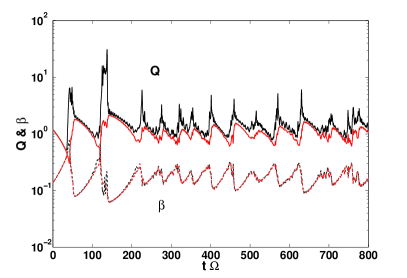
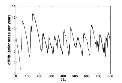
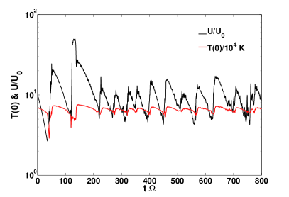
Figure 1: Time evolution of a shearing sheet at mean radius $r_{0}=10^{3}r_{s}$ about a $10^{8}M_{\odot}$ black hole, with mean surface density $\langle\Sigma\rangle_{A}=2\Sigma_{0}$, box size $10L_{0}\times 10L_{0}$, and resolution $256^{2}$. (See §2.4 for definitions of the units $L_{0}$ and $\Sigma_{0}$.) Panel (a), solid lines: Averaged Toomre parameters $\langle Q\rangle_{A}$ (black); $\langle Q\rangle_{M}$ (red). Dashed lines: averaged gas-pressure fractions $\langle\beta\rangle_{A}$ (black); $\langle\beta\rangle_{M}$ (red). Panel (b): Average accretion rate $\langle\dot{M}\rangle_{A}$ via eq. (30) [$M_{\odot}{\,\rm yr^{-1}}$]. Panel (c): Average cooling time $\langle t_{c}\rangle_{A}$ (red) and maximum surface density $\Sigma_{max}$ (black). Panel (d): Average internal energy per unit area $\langle U\rangle_{A}$ (black) mid-plane temperature $\langle T(0)\rangle_{A}$ (red). No permanent fragments form, so areal and mass-weighted averages $\langle\ldots\rangle_{A,M}$ are similar.

4.1 Case I: No permanent fragments

Figure 1 shows the evolution of several diagnostic quantities in a simulation for $r_{0}=10^{3}r_{s}$, $\Sigma_{i}=2\Sigma_{0}$, and $U_{i}=10U_{0}$. The quantities shown in the plots are implicitly averaged over the grid, and in some cases weighted by mass. When it is important to be explicit, we use angle brackets with appropriate subscripts, e.g.

$$\langle\beta\rangle_{A}=\frac{1}{L_{x}L_{y}}\iint\beta(x,y,t)\,dxdy\,,\qquad\langle\beta\rangle_{M}=\frac{1}{L_{x}L_{y}\langle\Sigma\rangle_{A}}\iint\Sigma\beta\,dxdy\,.$$ (36)

Occasionally overbars are used instead of brackets when we want to emphasize the time dependence of a spatial average, and we indicate by context or in some other way whether weighting by mass has been applied. Double brackets $\langle\langle\ldots\rangle\rangle_{A}$ or $\langle\langle\ldots\rangle\rangle_{M}$ will indicate averages over time as well as space.

In this notation, the areal average $\bar{\Sigma}(t)=\langle\Sigma\rangle_{A}=\Sigma_{i}$ since mass is conserved by our equations. For these choices of $r_{0}$ and $\bar{\Sigma}$ mentioned above, we find that a statistical steady state is reached after $t\sim 200\Omega^{-1}$ in which all of the quantities shown in Figure 1 fluctuate around long-term averages $\langle\langle\ldots\rangle\rangle$ that appear to be independent of the initial value $U_{i}$, as long as $U_{i}$ is not so low that the sheet immediately fragments without cooling. In particular, $\langle\langle Q\rangle\rangle_{A}\approx\langle\langle Q\rangle\rangle_{M}\approx 1$. Unless otherwise noted, we prefer to start from a hot state $Q_{i}\gg 1$.

To verify the steady state, we compare the cooling and heating rates. Averaged over the time interval between 200 $\Omega^{-1}$ and 800 $\Omega^{-1}$, the cooling time $\langle\langle t_{c}\rangle\rangle\approx 29.9\Omega^{-1}$, and the viscosity parameter $\langle\langle\alpha\rangle\rangle\approx 0.035$, so that $\langle\langle t_{c}\rangle\rangle\Omega\approx\langle\langle\alpha\rangle\rangle^{-1}$ as required by thermal equilibrium (§2.5). The accretion rate [Panel (b)] is somewhat larger than the Eddington rate $\dot{M}_{\rm Edd}=0.22M_{8}\epsilon^{-1}M_{\odot}{\,\rm yr^{-1}}$ for this black hole for canonical values of the global radiative efficency $\epsilon\equiv L_{\rm disk}/\dot{M}c^{2}\approx 10\%$. However, because $r_{0}$ enters the shearing-sheet equations only via $\Omega$, these results could be mapped to $r_{0}\approx 200r_{\rm S}$ around a $10^{9}M_{\odot}$ black hole, where the accretion rate would be sub-Eddington. Panel (c) shows occasional strong peaks in surface density; however $\langle Q\rangle$, which is a reciprocal measure of midplane density, never drops far below unity, showing that no permanent fragments form. Notice that the mass-weighted average $\langle Q\rangle_{M}$ is systematically less than the areal average $\langle Q\rangle_{A}$ because $\rho(0)$ correlates with $\Sigma$.

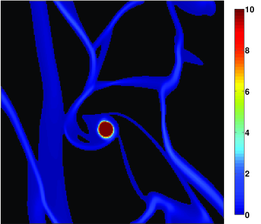
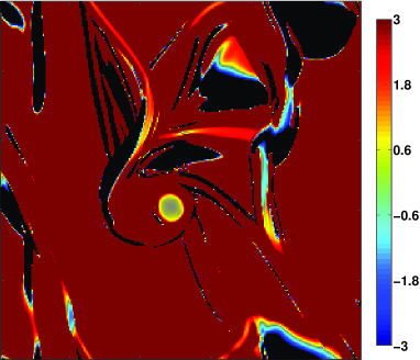
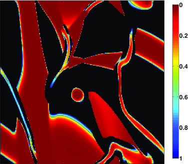
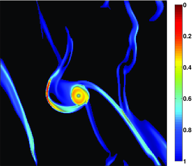
Figure 2: A bound fragment at $t=53\Omega^{-1}$ in a simulation for $r_{0}=4\times 10^{3}r_{s}$ and $\langle\Sigma\rangle_{A}=0.7\Sigma_{0}$. Clockwise from upper left: Surface density $\Sigma/\Sigma_{0}$; potential vorticity $\xi$ ($\xi=0.71$ in the initial uniform state); gas pressure fraction $\beta$; and local Toomre parameter $Q$ [eq. (4)].

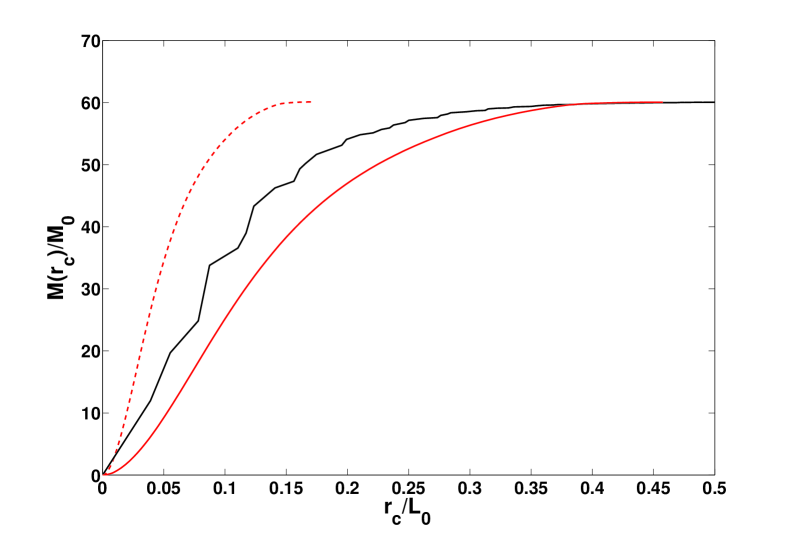
Figure 3: Black curve: Density profile of the fragment in Figure 2 versus distance $r_{c}$ from its center. Some $99.9\%$ of the bound mass lies at $r_{c}\leq 0.46L_{0}$, whereas the Hill radius for $600M_{\odot}$ is $\approx 1.46\,L_{0}$. Solid red curve: Radial profile an Eddington model of mass $60.1M_{0}$ and outer radius $0.46L_{0}$ projected into two dimensions. Dashed red curve: A projected Eddington model of the same mass having the same central surface density as the fragment. The object appears to be distended by a combination of rotation and numerically softened gravity.

4.2 Case II: Permanent fragments

In a constant-$\dot{M}$, constant-$\alpha$ disk, $Q$ declines with increasing radius (e.g. Goodman 2003), making fragmentation more likely. In a simulation with $\langle\Sigma\rangle_{A}=0.7\Sigma_{0}$ at $r_{0}=4\times 10^{3}r_{s}$, the disk cools to $Q<1$, and fragments form; as the sheet passes through $\langle Q\rangle_{A}=1$ the dimensionless cooling time $\Omega\langle t_{c}\rangle_{A}\approx 0.5$. Starting from a uniform state, the mass first concentrates into azimuthal filaments, which then fragment into several dense clouds. After merging, a single bound object containing most of the mass results from our standard $10L_{0}\times 10L_{0}$ simulation (Fig. 2). Unable to collide with itself, the object steadily cools. It shows no tendency to subfragment, as its Kelvin-Helmholtz time (21) is longer than $\Omega^{-1}$, which in turn is longer than its internal dynamical time.

No steady state results since we omit fusion reactions (which would ignite below the resolution of our grid). For the same $\langle\Sigma\rangle_{A}/\Sigma_{0}$, however, fragmention is avoided at the slightly larger radius $3\times 10^{3}r_{s}$, where we measure $\langle\langle\dot{M}\rangle\rangle\approx 2M_{\odot}{\,\rm yr^{-1}}$, congruent with an Eddington-limited disk feeding a $10^{8}M_{\odot}$ black hole at $10\%$ radiative efficiency.

Figure 2 displays the fragmenting simulation at $t=53\Omega^{-1}$, after the dominant fragment has coalesced. As shown by the lower left panel, $Q\ll 1$ within the fragment, meaning that its midplane density is well above the Roche value. About half of the rest of the sheet is also dense at the midplane, but these regions have very little mass. The mass in the bound object is about $60M_{0}\approx 614M_{\odot}$, $86\%$ of the total. At this time, $\langle\langle Q\rangle\rangle_{M}\approx 0.019$, and $\langle\langle\beta\rangle\rangle_{M}\approx 0.45$. Note that this $\beta$ is larger than what we expect for a nonrotating Eddington model of the same mass (eq. 23). This may in part be a numerical effect of our finite spatial resolution, which softens the gravitational force: as the radial density profile in Fig. 3) shows, the half-mass radius of the object is approximately two cell widths. Another cause of the discrepancy may be the large rotational kinetic energy of this object, $T/|W|\approx 0.13$.

The energy of this object is partitioned as follows: thermal energy $E_{\rm th}=936E_{0}$; kinetic energy (measured with respect to its center of mass, mainly rotational) $E_{k}=672E_{0}$; tidal potential energy $E_{t}=-0.8E_{0}$; gravitational self-energy $E_{p}=-5060E_{0}$. Thus the total energy of the object in its center-of-mass frame is negative, implying that the object is bound and doomed to contract indefinitely.

Our 2D approximation facilitates merging because fragments cannot avoid one another vertically. The importance of this can be judged by examining the epicyclic motions of fragments, if one is willing to assume that the vertical and horizontal epicyclic amplitudes scale together. The epicyclic energy per unit mass of a free particle in the Keplerian shearing sheet is $\dot{x}^{2}+(2\dot{y}+3\Omega x)^{2}$ is a constant. For an isolated fragment, the corresponding characteristic quantity is

$$E_{\text{epi}}=\frac{1}{2}M\left[\bar{v}_{x}^{2}+(2\bar{v}_{y}+3\Omega\bar{x})^{2}\right].$$ (37)

Here $M$ is the mass of the fragment, while the overbars mark the position and velocity of its center-of-mass. We define the (radial) epicyclic amplitude by $R_{\text{epi}}\equiv\sqrt{2E_{\text{epi}}/(M\Omega^{2})}$. The importance of the third dimension for collisions can be judged by comparing $R_{\text{epi}}$ to the physical radius of the object, $R_{*}$, or to its Hill radius, $R_{H}$ [eq. (28)]. We presume that the latter is the more relevant comparison, at least until $R_{*}/R_{H}\lesssim 0.1$, because objects within one another’s Hill sphere undergo a complicated motion in 3D that allows many opportunities for close passage.

At $t=48.4\Omega^{-1}$ in the above-described simulation for $r_{0}=4\times 10^{3}r_{s}$, there are two fragments, with masses $50.6M_{0}$ and $2M_{0}$, so that the Hill radius associated with their combined masses is $R_{H}\approx 1.4\,L_{0}$. The epicyclic amplitude for the smaller mass is $R_{\text{epi}}\approx 3.14L_{0}$. Later in our 2D simulation, these two fragments merge. We conclude that the merger might have been delayed or perhaps even avoided in 3D.

In order to explore merging among more fragments, we have performed a simulation for the same $r_{0}$, $\langle\Sigma\rangle_{A}$, and resolution as in Figure 2 but with four times the standard box size, i.e. $L_{x}=L_{y}=40L_{0}$ and $NX=NY=1024$. The first bound fragments appear at $t\approx 13\Omega^{-1}$. Along one filament, fourteen small fragments form, and eight merge in pairs. It is easily shown the two-body problem decomposes in the shearing sheet into uncoupled motions of the center-of-mass and relative coordinates, as in free space. Therefore, adopting the approximation that the epicyclic motions of the two components of each pair are uncorrelated until shortly before they merge, we add their epicyclic amplitudes in quadrature, $r_{\rm epi}=(r_{\rm epi,1}^{2}+r_{\rm epi,2}^{2})^{1/2}$, and compare this to the Hill radius based on their combined mass, $R_{\rm H}=[G(m_{1}+m_{2})/3\Omega^{2}]^{1/3}$, with the results shown in Table 1.

$(m_{1}+m_{2})/M_{0}$	$m_{2}/m_{1}$	$r_{\rm epi}/R_{\rm H}$
2.17	0.61	3.10
3.17	0.83	2.40
1.37	0.99	1.15
1.43	0.96	1.68

Table 1: Epicyclic amplitudes of merging pairs.

The data in the last column suggest that these encounters might have proceeded somewhat differently in three dimensions.

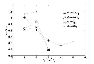
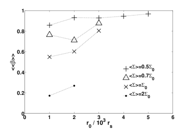
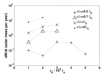
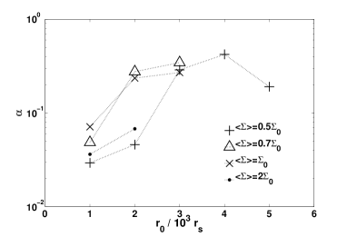
Figure 4: Derived properties of statistically steady, nonfragmenting simulations versus radius and scaled surface density [$\hat{\Sigma}$; eqs. (25) & (29)], for $M_{\rm{BH}}=10^{8}M_{\odot}$. The various symbol types mark corresponding simulations in all four panels. The cases for $\hat{\Sigma}=1,2$ fragment beyond $2\times 10^{3}r_{\rm S}$ & $3\times 10^{3}r_{\rm S}$, respectively, hence are not shown. The averages of $Q$ and $\beta$ [panels (a) &(b)] are mass-weighted and systematically smaller than the corresponding areal averages.

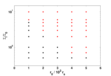
Figure 5: The fragmentation boundary. Panel (a): Red dots mark simulations that fragmented, black dots mark those that did not. Panel (b): $\dot{M}$ (solid line) and $\alpha$ (dashed line) along the fragmentation boundary, i.e. for the uppermost black dots in Panel (a). These represent maximal rates of gravitational transport without fragmentation. For $\beta_{1}$ & $t_{\rm c,1}$, see the text.

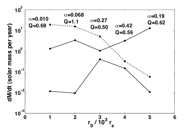
Figure 6: Comparison of $\dot{M}$ along the fragmentation boundary with G03. Dashed curve: As in Panel (b) of Fig. (5). Solid curves: Predicted values of $\dot{M}$ for the indicated $Q$ & $\alpha$ taken from the simulations, using eqs. (11) & (A3) of G03.

4.3 General picture of the self-gravitating regime

In this section, we summarize the general trends found in our shearing-sheet models, with particular attention to the conditions for fragmentation.

As discussed above, the eventual statistical steady state of our simulations, when it exists, are defined by two control parameters, mean surface density, $\langle\Sigma\rangle$, and angular velocity, $\Omega=(GM_{\rm{BH}}/r_{0}^{3})^{1/2}$. We have explored the parameter ranges $0.5\Sigma_{0}\leq\langle\Sigma\rangle\leq 10\Sigma_{0}$ and $10^{3}r_{\rm S}\leq r_{0}\leq 5\times 10^{3}$, with $M_{\rm{BH}}=10^{8}M_{\odot}$. Throughout most of this regime, the effective Shakura-Sunyaev parameter is measured to be $\alpha\gtrsim 10^{-2}$, so that self-gravity would likely have dominated the angular momentum transport even had we included MHD in our simulations. The corresponding accretion rates are $0.01\lesssim\dot{M}\lesssim 20\ M_{\odot}\ \mbox{yr}^{-1}$.

Figure 4 shows several steady-state quantities as functions of our two control parameters. With the physics in our models, steady states are not possible after fragmentation, so these quantities are measured from simulations that did not fragment. As seen in the first panel, the mass-weighted average of $Q$ is typically slightly less than $\lesssim 1$. Recall that our definition of $Q$ [eq. (4)] is simply a reciprocal measure of the midplane density relative to the Roche density; under adiabatic compression by a nonlinear density wave, the internal energy of the gas rises in step with its density, so that a bound fragment may be avoided even if $Q$ falls briefly below unity. Mass weighting tends to emphasize these transiently compressed regions. The areal average of $Q$ is typically $\gtrsim 1$. At a given $\hat{\Sigma}=\langle\Sigma/\Sigma_{0}\rangle$, $Q$ decreases toward larger radii, where cooling is stronger. Panel (b) shows that the mass-weighted $\beta$ increases with increasing radius and decreasing surface density. Panel (c) shows that $\dot{M}$ is much more sensitive to surface density ($\hat{\Sigma}$) than to radius or, equivalently, to $\Omega$. For comparison, the Eddington rate for a black hole of $10^{8}M_{8}\,M_{\odot}$ is $\dot{M}_{\rm Edd}\approx 2M_{8}\epsilon_{0.1}M_{\odot}\ \mbox{yr}^{-1}$, where $\epsilon=0.1\epsilon_{0.1}\equiv L_{\rm disk}/\dot{M}c^{2}$ is the global radiative efficiency of the disk. For $\hat{\Sigma}=1$, the Eddington rate is achieved at $r_{0}\approx 3\times 10^{3}r_{s}$. At the same $\dot{M}$, however, our models fragment when $r_{0}\gtrsim 4\times 10^{3}r_{s}$. The final panel shows that generally $\alpha$ increases with increasing radius at fixed $\hat{\Sigma}$. But $\alpha$ has a complicated dependence on surface density. The largest value encountered in any of our non-fragmenting simulations was $\alpha_{\max}\approx 0.4$.

Figure 5 shows the boundary between those cases that fragment and those that do not in the plane of $(r_{0},\hat{\Sigma})$, our two control parameters. Each dot represents a simulation, all done with $L_{x}=L_{y}=10L_{0}$ and $NX=NY=256$. We have checked that the boundary between the fragmenting (red) and nonfragmenting (black) cases is not significantly altered at higher resolution ($NX=NY=512$). Higher resolution does make a difference, however, when the most unstable wavelength is short, which happens when the accretion rate (and thus surface density) is very small: our standard resolution begins to fail at $\dot{M}<0.1M_{\odot}\ \mbox{yr}^{-1}$.

Panel (a) of Figure 5 shows that the maximum dimensionless surface density that the disk can support without fragmenting declines rapidly with increasing radius. Over the range $10^{3}\leq r_{0}/r_{\rm S}\leq 4\times 10^{3}$, the boundary can be fit to a power law: $\hat{\Sigma}_{\rm frag}\approx 6(r/10^{3}r_{\rm S})^{-1.5}$. Since, as shown in Figure 4, the local accretion rate is much more sensitive to $\hat{\Sigma}$ than to $r_{0}$, it follows that $\dot{M}_{\rm max}$ also declines swiftly with radius; this is confirmed by the second panel. In fact, $\dot{M}_{\max}$ declines some two orders of magnitude between $10^{3}r_{\rm S}$ and $5\times 10^{3}r_{\rm S}$.

The gas pressure fraction $\beta_{1}$ and cooling time $t_{\rm c,1}$ marked in the second panel are neither mass-weighted nor areal averages: instead, they are computed for the same $r_{0}$ and $\langle\hat{\Sigma}\rangle$ as those in the simulation, but with $Q$ set to unity in the equation of state rather than its measured steady-state value. This allows us to compare the observed fragmentation boundary with Gammie’s criterion $(\Omega t_{\rm c})_{\rm crit}=\mbox{constant}=O(1)$. Except at the innermost radius shown, we find that the cooling time is indeed $O(\Omega^{-1})$ along the boundary. However, fragmentation occurs at $r=10^{3}r_{\rm S}$ when $\langle\hat{\Sigma}\rangle\gtrsim 5$ even though $\Omega t_{\rm c}\gg 1$; this is possible because $\beta\ll 1$, so that bound fragments are only marginally stable against collapse even without energy loss. For $M_{\rm{BH}}=10^{8}M_{\odot}$, this regime is reached only at local accretion rates far above the Eddington rate, but not so for larger $M_{\rm{BH}}$, as will be shown in §4.4.

We have compared our simulations with the alpha-disk models of G03 for the case that viscosity is proportional to total pressure. Figure 1 of G03 displays curves of constant $\alpha$ and $Q$ in a plane of $\dot{M}$ versus $r$. For $Q=1$ and plausible $\alpha$, there are generally two branches to the curve: a high-$\dot{M}$ solution, which has high surface density and low $\beta$, and a low-$\dot{M}$ solution, which has the oppositie properties. These branches join at $r\approx 10^{3}r_{\rm S}$, so that $Q>1$ for all solutions at smaller radii. To compare with these predictions, we take the measured values of $\alpha$ and mass-weighted $Q$ from the simulations along the fragmentation boundary shown in Panel (b) of Fig. 5, and we insert these values into the model for $\dot{M}$ from G03. The results are shown by solid lines in Fig. 6. There are again two solutions for $\dot{M}$ at each radius, with radiation pressure dominating the upper (higher $\dot{M}$) solution, and gas pressure dominating the lower. But while $Q$ is roughly constant along these curves, $\alpha$ is not—$\alpha$ decreases rapidly with decreasing radius. The actual $\dot{M}$ directly measured in the simulations (dashed curve) lies above the upper branch at $r<4\times 10^{3}r_{\rm S}$ and has slightly higher surface density. The differences between the predicted and measured values of $\dot{M}$ may be due in part to the assumption of uniform conditions in the $\alpha$ models, so that mass and areal averages differ.

4.3.1 Scaling to other black-hole masses

Apart from fundamental constants and numerical parameters (grid resolution, domain size, etc.), the statistical steady states of our self-gravitating shearing sheets are entirely determined by just two control parameters: $\Omega$ and $\langle\Sigma\rangle$. Therefore, although we have fixed $M_{\rm{BH}}=10^{8}M_{\odot}$ in our simulations and studied the outcomes as functions of $r_{0}$ and $\langle\hat{\Sigma}\rangle$, we can scale our results to other black-hole masses by recasting them in terms of the two control parameters above. For ease of writing, we will omit the angle brackets from $\langle\Sigma\rangle$ and $\langle\hat{\Sigma}\rangle$ henceforth.

Our most important result is the fragmentation boundary. As noted above, $\hat{\Sigma}_{\rm frag}\approx 6r_{3}^{-x}$, with $x\approx 1.5$. Since $r_{\rm S}\propto M_{\rm{BH}}$ and $\Sigma_{0}\propto\Omega^{4/3}$ [eq. (25)], this can be recast as

$$\Sigma_{\rm frag}\approx 2\times 10^{6}\left(M_{8}^{2/3}r_{3}\right)^{-(2+x)}\,{\rm g\,cm^{-2}}\,.$$ (38)

We compare this with the surface density required for accretion at the Eddington rate. From Panel (c) of Fig. 4, it appears that $\dot{M}$ is much more sensitive to $\hat{\Sigma}$ than to radius. This implies that $\Sigma\propto r^{-2}$ at fixed $\dot{M}$. We will attempt to explain this scaling below, but for the moment, we simply accept it. Since $\dot{M}$ increases by a factor $\approx 10^{2}$ as $\hat{\Sigma}$ increases by $4$, we estimate $\dot{M}\propto\hat{\Sigma}^{y}$ with $y\approx 3.3$. Figure 4 also indicates that $\hat{\Sigma}\approx 0.7$ yields $\dot{M}\approx 2{\rm\,M_{\odot}\,yr^{-1}}$, which is the Eddington rate for $M_{\rm{BH}}=10^{8}{\rm\,M_{\odot}}$ and radiative efficiency $\epsilon=0.1$. This coincides with $\Sigma_{\rm frag}$ at $r_{3}\approx 4$ for $M_{8}=1$. Rewriting the relation $\dot{M}\approx 2{\rm\,M_{\odot}\,yr^{-1}}(\hat{\Sigma}/0.7)^{y}$ as $\dot{M}\propto(\Sigma\Omega^{4/3})^{y}$, we find that the radius beyond which a self-gravitating accretion disk will fragment if it accretes at a fraction $\dot{m}$ of the Eddington rate is, taking $x=1.5$ and $y=3.3$,

$$r_{\rm crit} \approx 4\times 10^{3}M_{8}^{-0.87}\dot{m}^{0.2}r_{\rm S}\quad\approx 0.04\,M_{8}^{0.13}\dot{m}^{0.2}\,{\rm pc}.$$ (39)

For comparision, Goodman (2003)’s equation (10) predicts that $Q=1$ in an alpha disk at $r_{3}\approx 2.7(\alpha/M_{8})^{2/9}$ if the viscous stress is proportional to total pressure and $\beta\ll 1$. This is roughly half of eq. (39) for $M_{8}=1$ and $\alpha=0.4$ (the largest value found in our simulations), but the scaling with black-hole mass is different. As Panel (b) of Figure 4 shows, however, $\beta$ is closer to 1 than to 0 at $r_{\rm crit}$ for $M_{8}=1$, so precise agreement is not to be expected.

We promised to discuss why $\Sigma\propto r^{-2}$ at fixed $\dot{M}$ and $M_{\rm{BH}}$. When self-gravity controls the accretion rate, $Q\approx 1$, so that the midplane density $\rho(0)\propto r^{-3}$. It follows from vertical radiative and hydrostatic equilibrium that the half thickness of the disk is

$$h\approx\frac{3\kappa\dot{M}}{8\pi c}(1+2Q^{-1})^{-1}(1-\beta)^{-1}$$ (40)

to the extent that $\beta$ is vertically constant. This gives the familiar result that $h\approx\mbox{constant}$ in steady disks where radiation pressure dominates. Then we would have $\Sigma=2h\rho(0)\propto r^{-3}$, not $r^{-2}$, for constant $Q$. Fig. 4 shows, however, that $\beta\gtrsim 0.7$ at $r_{3}\geq 1$ for $\hat{\Sigma}=0.7$, the value that gives a roughly Eddington accretion rate for $M_{8}=1$. Thus $h$ may vary with radius through the factor $(1-\beta)^{-1}$. Now eq. (A3) of Goodman (2003) predicts that

$$(1-\beta)^{-1}\beta^{1/2+(b-1)/10}\approx 0.35(\alpha_{0.1}M_{8})^{-1/10}\dot{m}^{-4/5}\left(\frac{\kappa}{\kappa_{\rm es}}\right)^{-9/10}r_{3}^{21/20}\,,$$ (41)

where $b=0$ or $b=1$ according as $\nu\propto P$ or $\nu\propto P_{\rm rad}$: clearly it makes little difference to the value of $(1-\beta)$ when this is $\lesssim 0.5$. Although $\alpha$ is not constant with radius in our self-gravitating models, the dependence in eq. (41) is so weak that $(1-\beta)^{-1}$ and hence $h$ are approximately linear in $r$ when $\beta\gtrsim 0.5$. This explains why $\Sigma\propto r^{-2}$, but it also shows that this scaling holds only over a limited range of $r$ and $M_{\rm{BH}}$.

Equation (39) shows that self-gravity is important at a smaller multiple of $r_{\rm S}$ for larger $M_{\rm{BH}}$ at a given Eddington fraction $\dot{m}$; it then follows from eq. (41) that the self-gravitating regime is characterized by smaller $\beta$ for larger $M_{\rm{BH}}$. In fact, for $M_{\rm{BH}}\gtrsim 10^{9}{\rm\,M_{\odot}}$, we estimate that $\beta<0.1$ at $r_{\rm crit}$, so that fragmentation may occur with little cooling, as demonstrated in §4.4. Thus, while it remains true that the local dynamics of a self-gravitating disk is determined by $\Omega$ and $\Sigma$, the particular scaling (39), which depends upon our power-law fit to the fragmentation boundary over a limited range of $\beta$, is likely to be modified for black-hole masses much above $10^{8}{\rm\,M_{\odot}}$. On the other hand, for black holes much less massive than our fiducial value, Kramer’s opacity will dominate over electron scattering at $r_{\rm crit}$; in view of the sensitivity of the radiation fraction (41) to $\kappa$, this also will modify eq. (39). Thus, the latter equation is probably quantitatively reliable within only a narrow range around $M_{8}=1$. Nevertheless, the trend is surely correct: namely, that $r_{\rm crit}$, the radius beyond which accretion at the Eddington rate would cause fragmentation, occurs at a smaller multiple of $r_{\rm S}$ for larger $M_{\rm{BH}}$.

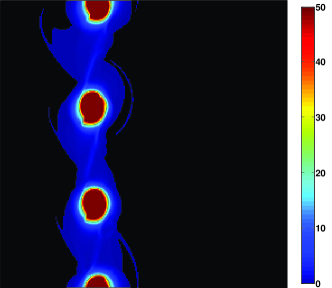
(a) $t\Omega=53$

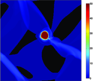
(b) $t\Omega=60$

Figure 7: Simulation for $r_{0}=621r_{s}$, $\langle\Sigma\rangle_{A}=9.6\Sigma_{0}$ of $10^{9}M_{\odot}$ SMBH. Line plots: Evolution history of accretion rate calculated from eq. (30), $\alpha$, and mass-weighted $Q$ and $\beta$. Because the disk is not in thermal balance, the $\dot{M}$ shown here does not reflect that due to turbulent stress, which would be smaller. Lower left: Three fragments form at time $t=53\Omega^{-1}$. Lower right: A single fragment is left after mergers at time $t=60\Omega^{-1}$.

4.4 Fragmentation at long cooling times

As noted in §1, the softening influence of radiation pressure on the equation of state may allow fragmentation even for $\Omega t_{c}\gg 1$. One way to enter this regime is to increase the mean surface density. At fixed radius and fixed $Q$, the gas pressure fraction $\beta\approx 0.5\hat{\Sigma}^{-3/2}$ [eq. A8], while the cooling time $t_{c}\propto\kappa\hat{\Sigma}^{2}$. For example, with $Q=1$ and $\hat{\Sigma}=6$ at $r_{0}=10^{3}r_{s}$ and $M_{\rm{BH}}=10^{8}M_{\odot}$, our equation of state yields $\beta=0.03$ and $\Omega t_{\rm c}=244$. At $r_{0}\lesssim 200r_{s}$ along the fragmentation boundary shown in Fig. 5, $\beta$ is already very small and $t_{c}\Omega$ is large. The surface density exceeds what is required to support the Eddington luminosity but might occur if mass were dumped into the disk by a violent event such as a merger.

Another way to enter this regime is by increasing the mass of the black hole at a fixed Eddington fraction, $\dot{m}$. At $M_{\rm{BH}}=10^{9}M_{\odot}$ and $\dot{m}=1$, the disk is still strongly dominated by radiation pressure at the smallest radii where self-gravity is important. Setting $l_{\rm E}/\epsilon_{0.1}\equiv\dot{m}=1$, $M_{8}=10$, and $\alpha=0.01$ in equations (A2)-(A4) of G03, we estimate that $Q=1$ occurs at $r_{0}=621r_{s}$, where $\beta=0.02$ and $\hat{\Sigma}=9.6$.

We have done one simulation with these values of $M_{\rm{BH}}$, $r_{0}$, and $\hat{\Sigma}$ (Figure 7). The simulation starts at $Q=1.2$ and cooling time $t_{c}\Omega=49$. The large but declining values of $\dot{M}$ in the first panel are computed from the thermal equation (30) rather than the stress equation (32), which would predict $\dot{M}\approx 0$ in the initial phases when $\alpha\approx 0$. A sustained balance between radiative cooling and turbulent heating is never achieved, even though the cooling is slow and proceeds smoothly to $Q<1$. After roughly one cooling time, at $t\approx 50\Omega^{-1}$, the sheet collapses to an azimuthal filament. This quickly breaks into three massive fragments, which merge into one at $60\Omega^{-1}$. The energies of the final object are $E_{\rm th}=4.6\times 10^{5}E_{0}$, $E_{\rm kin}=7.5\times 10^{4}E_{0}$, $E_{\rm tid}=-15.1E_{0}$, and $E_{\rm grav}=-5.4\times 10^{5}E_{0}$, respectively, so that it is marginally bound.

As this example shows, the mass scale for fragmentation is very large if it occurs at $\beta\ll 1$. This is to be expected from the Eddington quartic (23). The fragments inherit an initial $\beta$ similar to that of the disk because their formation occurs roughly adiabatically at high specific entropy, $T^{3}/\rho\approx\mbox{constant}$. The final object weighs $893M_{0}\approx 9000M_{\odot}$ at $\langle\beta\rangle_{m}\approx 0.07$, close to the prediction from eq. (23) but larger than the value $\beta_{\rm disk}\approx 0.02$ expected for a uniform sheet at $Q=1$ with this mean surface density.

We have not attempted a thorough a survey of parameter space for $M_{\rm{BH}}=10^{9}M_{\odot}$ as we did for $10^{8}M_{\odot}$. One obstacle is that the cooling time becomes very long, especially at small radii. Another is that the gravitational stress remains small up to the point of fragmentation, in contrast to the situation for $10^{8}M_{\rm{BH}}$ where $\alpha_{\max}\approx 0.4$ (Fig. 5). At $\alpha\lesssim 10^{-2}$, heating by MRI becomes important, which cannot be explored with this 2D code. MRI might have prevented fragmentation for the disk parameters of Fig. 7, since $Q\geq 1$ is predicted for these parameters if $\alpha\geq 10^{-2}$, and fragmentation did not begin until $Q\lesssim 0.5$. The point, however, is that self-gravity alone was not able to supply a sufficiently large $\alpha$ despite the long cooling time. Thus our simulations demonstrate that fragmentation can occur at dimensionless cooling times $\Omega t_{\rm c}\gg 1$ when radiation pressure dominates, $\beta\ll 1$.

5 Discussion and Conclusions

Radiation pressure and appropriate opacities are part of the minimal physics needed to study gravitational turbulence and fragmentation in near-Eddington AGN accretion disks. We have included these and used them to test the predictions of Goodman (2003) for the maximum radius at which AGN disks can support steady accretion at the Eddington rate without fragmentation. We are in qualitative agreement with that paper, but quantitatively we find that the critical radius is about twice as large as was predicted for $M_{\rm{BH}}=10^{8}{\rm\,M_{\odot}}$. We are also generally in agreement with Gammie (2001)’s criterion for fragmentation, except that fragmentation may occur for $\Omega t_{\rm cool}\gg 1$ if radiation pressure dominates.

Beyond this, however, our local 2D approximation limits what we can explore and what we can conclude. Magnetohydrodynamic (MHD) and magnetorotational (MRI) processes cannot be represented, at least not directly. This probably does not much alter the conditions for marginal fragmentation, because the effective viscosity due to self-gravity is much larger in this regime than what MRI can provide. We cannot, however, exclude the possibility that MRI, or some other effective viscosity that does not respect the conservation of specific vorticity, might interact with the self-gravity in subtle ways, for example by promoting secular instabilities at $Q>1$, or by enabling transitions among states of different $\dot{M}$ at the same $\Sigma$ and $\Omega$; we saw evidence for the latter behavior when we added an ad-hoc viscosity $\nu\propto P_{\rm gas}$ to our code, but we have not been able to understand those results and therefore have not presented them here. Our approximations also cannot represent magnetized winds or global spiral arms, which might in principle remove angular momentum at rates enhanced by $\sim r/h$ compared to transport within the disk, allowing a lower and hence less self-gravitating surface density for the same accretion rate (Goodman, 2003; Thompson et al., 2005; Hopkins & Quataert, 2010a).

Nor can we test Goodman & Tan (2004)’s suggestion that fragments grow rapidly up to the isolation mass, which is typically $\sim 10^{5}{\rm\,M_{\odot}}$. There are two principal obstacles. One is numerical: very large self-gravitating masses are very strongly radiation-pressure dominated, and therefore only marginally bound when in virial equilibrium, so that small energy errors can cause spurious expansion or collapse. This is likely to be a difficulty for many numerical algorithms besides ZEUS in low-$\beta$, self-gravitating regimes. The second is physical: our 2D results show that in shearing sheets where multiple bound fragments are present, the gravitational interactions between fragments quickly increases their epicyclic motions to amplitudes exceeding their Hill radii, so that they would be expected to scatter into the third dimension if that were allowed (Rafikov & Slepian, 2010).

Notwithstanding these limitations of 2D, our results strongly suggest that if the disks of bright QSOs extend at constant $\dot{M}$ to $\gtrsim 0.01\mbox{-}0.1{\rm\,pc}$, then bound objects will form with individual masses of at least $300M_{\odot}$, and possibly much more. Collectively, these “stars” will dominate the local surface density of the disk, though they may be accompanied by an optically thick layer of distributed gas. The stars will attain epicyclic dispersions bounded by Safronov numbers $\Theta\equiv GM_{*}/(R_{*}\sigma_{r,\rm epi}^{2})\lesssim 1$, so that even if they contract to their main-sequence radii and are stable enough to remain there, $(M_{*}/M_{\rm{BH}})(r/R_{*})\ll 1$ unless $M_{*}\gtrsim 10^{5}{\rm\,M_{\odot}}$ (see Goodman & Tan 2004 for a review of the nominal main-sequence properties of very massive stars). Physical collisions will be important unless or until the objects collapse to black holes. One is thus lead to imagine a model for the disk similar to that advanced long ago by Spitzer & Saslaw (1966), and more recently by Miralda-Escudé & Kollmeier (2006). We imagine formation of (very massive) stars within a disk, however, rather than formation of a disk from a pre-existing dense nuclear star cluster.

Are there any observational signatures of such a fragmented disk that might distinguish it from the conventionally imagined smooth one? One such signature may be the super-solar metallicity inferred from the broad lines, which appears not to correlate with the general star formation rate in the host traced by far-infrared emission (Simon & Hamann, 2010), and therefore may implicate formation within the nuclear disk itself. Another signature might be deviations from the spectral energy distribution expected from a steadily accreting, optically thick disk. Goodman & Tan (2004) pointed out that the viscous accretion time at $r\sim 10^{3}r_{\rm S}$ is typically somewhat less than the minimum main-sequence lifetime, so that massive stars formed there might—if they are sufficiently stable—migrate to the inner edge of the disk before dying. In that case, if these stars dominate the surface density and are not fully enshrouded by diffuse gas, the local color temperature of the disk might be intermediate between that of the stars themselves and the effective temperature implied by the accretion rate. Gravitational microlensing observations are beginning to test the variation of apparent disk size with wavelength on relevant lengthscales; the evidence is consistent with color temperature $\propto r^{-3/4}$ as expected for steady, optically thick disks, but suggests that the disks are larger at a given wavelength than expected (Pooley et al., 2007; Morgan et al., 2010).

Appendix A Effective 2D Equation of State for vertically constant $\beta$

Vertical hydrostatic equilibrium in the combined gravitational fields of the central mass and of the disk itself is described by

$$\frac{1}{\rho}\frac{dp}{dz}=-\Omega^{2}z-4\pi G\int_{0}^{z}\rho(z^{\prime})dz^{\prime}\,,$$ (A1)

Putting $p=K(\beta)\rho^{4/3}$ [eq. (3)] and adopting the dimensionless Emden variables

$$\rho(z)=\rho(0)\theta^{3},\qquad\xi=z/h,\qquad h^{2}=\frac{K}{\pi G\rho(0)^{2/3}}\,,$$ (A2)

leads to

$$\frac{d^{2}\theta}{d\xi^{2}}+\theta^{3}=-\frac{\Omega^{2}}{4\pi G\rho(0)}\equiv-\frac{Q}{2}\,.$$ (A3)

Using the initial conditions $\theta(0)=1$ and $\theta^{\prime}(0)=0$, eq. (A3) can be reduced to a quadrature:

$$\xi=2\sqrt{2}\int_{0}^{\sqrt{1-\theta}}\frac{dw}{\sqrt{2Q+1+(1-w^{2})+(1-W^{2})^{2}+(1-w^{2})^{3}}}.$$ (A4)

The height-integrated density and pressure become

$$\Sigma=4\sqrt{2}\rho(0)hI_{3}(Q),\qquad P=4\sqrt{2}K(\beta)\rho(0)^{4/3}hI_{4}(Q),$$ (A5)

in which

$$I_{k}(Q)\equiv\int_{0}^{1}\frac{(1-w^{2})^{k}dw}{\sqrt{2Q+1+(1-w^{2})+(1-w^{2})^{2}+(1-w^{2})^{3}}},\qquad k=3,4.$$ (A6)

For all $w\in[0,1]$ and $Q\geq 0$, the denominators of the elliptic integrals (A6) vary by at most a factor of 2. Hence we approximate these integrals with single-point Gaussian quadrature scheme,

$$\int_{0}^{1}(1-w^{2})^{k}f(w^{2})dk\approx u_{k}(w_{k}^{2}),$$ (A7)

in which the point $w_{k}\in[0,1]$ and the weight $u_{k}>0$ are chosen so as to make this scheme exact for functions $f(w^{2})=A+Bw^{2}$ with arbitrary constants $A$ and $B$. For $k=3$ and $k=4$, the two integrals are close enough that the same value of $w_{k}$ can be used for both; this leads to the approximations (8), which are accurate to $\lesssim 1\%$ for all $Q\geq 0$. In practice, we prepare a table with a certain range of $\Sigma$ and $U$, within which we calculate the integrals (A6) directly. For conditions outside the table, the code uses the approximations (8).

Eliminating $h$ between eqs. (A2) and the first of eqs. (A5) and then expressing $\rho(0)$ in terms of $Q$ via eq. (4) leads to eq. (6). Using this to eliminate $K$ and $h$ from the second of eqs. (A5) then yields equation (5) for $P$ in terms of $Q$ and $\Sigma$. But $P$ is related to the internal energy by eq. (9), so (5) can be recast as (7). Finally, after replacing $K$ with its explicit form (3), equations (6) and (7) can be rewritten in terms of the dimensionless variables introduced in §2.4 as

$$\frac{2^{15}(1-\beta)}{\beta^{4}}=\frac{\pi^{3}Q^{4}}{\left[I_{3}(Q)\right]^{6}}\hat{\Sigma}^{6},\qquad\beta=2-\frac{128\left[I_{3}(Q)\right]^{3}}{3QI_{4}(Q)}\frac{\hat{U}}{\hat{\Sigma}^{3}}.$$ (A8)

Equations (A8) implicitly determine $\beta$ and $Q$ given $\hat{U}$ and $\hat{\Sigma}$, as exemplified by Fig. 8, after which $P$ follows from eqs. (9) or (5).

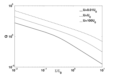
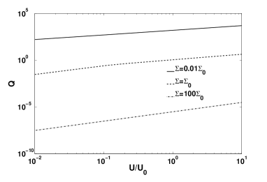
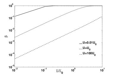
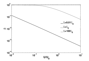
Figure 8: Solutions to equation (A8) for $\beta$ and $Q$ in the parameter space $\hat{\Sigma}$ and $\hat{U}$. In panel (a) and (c), we show the behavior of $Q$ and $\beta$ as a function of $\hat{\Sigma}$ for a fixed value of $\hat{U}$. Different lines are for different values of $\hat{U}$ as shown in the plots. In panel (b) and (d), we show the behavior of $Q$ and $\beta$ as a function of $\hat{U}$ for a fixed value of $\hat{\Sigma}$. The values of $\hat{\Sigma}$ for different lines are also shown in the plots. The four plots are the equation of state that we use in our code.

References

- Bartko et al. (2010) Bartko, H., et al. 2010, ApJ, 708, 834
- Bond et al. (1984) Bond, J. R., Arnett, W. D., & Carr, B. J. 1984, ApJ, 280, 825
- Collin & Zahn (1999) Collin, S., & Zahn, J. 1999, A&A, 344, 433
- Davies et al. (2007) Davies, R. I., Sánchez, F. M., Genzel, R., Tacconi, L. J., Hicks, E. K. S., Friedrich, S., & Sternberg, A. 2007, ApJ, 671, 1388
- Dhanda et al. (2007) Dhanda, N., Baldwin, J. A., Bentz, M. C., & Osmer, P. S. 2007, ApJ, 658, 804
- Gammie (2001) Gammie, C. F. 2001, ApJ, 553, 174
- Ghez et al. (2003) Ghez, A. M., et al. 2003, ApJ, 586, L127
- Goodman (2003) Goodman, J. 2003, MNRAS, 339, 937, (G03)
- Goodman & Tan (2004) Goodman, J., & Tan, J. C. 2004, ApJ, 608, 108
- Hamann & Ferland (1993) Hamann, F., & Ferland, G. 1993, ApJ, 418, 11
- Hawley et al. (1995) Hawley, J. F., Gammie, C. F., & Balbus, S. A. 1995, ApJ, 440, 742
- Hirose et al. (2009) Hirose, S., Blaes, O., & Krolik, J. H. 2009, ApJ, 704, 781
- Hopkins & Quataert (2010a) Hopkins, P. F., & Quataert, E. 2010a, ArXiv e-prints
- Hopkins & Quataert (2010b) —. 2010b, MNRAS, 1085
- Hubeny (1990) Hubeny, I. 1990, ApJ, 351, 632
- Johnson & Gammie (2003) Johnson, B. M., & Gammie, C. F. 2003, ApJ, 597, 131
- Kuo et al. (2010) Kuo, C. Y., et al. 2010, ArXiv e-prints
- Lauer et al. (2005) Lauer, T. R., et al. 2005, AJ, 129, 2138
- Lee & Goodman (1999) Lee, E., & Goodman, J. 1999, MNRAS, 308, 984
- Lightman & Eardley (1974) Lightman, A. P., & Eardley, D. M. 1974, ApJ, 187, L1+
- Lodato & Rice (2004) Lodato, G., & Rice, W. K. M. 2004, MNRAS, 351, 630
- Martins et al. (2008) Martins, F., Gillessen, S., Eisenhauer, F., Genzel, R., Ott, T., & Trippe, S. 2008, ApJ, 672, L119
- Masset (2000) Masset, F. 2000, A&AS, 141, 165
- Miller & Antonucci (1983) Miller, J. S., & Antonucci, R. R. J. 1983, ApJ, 271, L7
- Miralda-Escudé & Kollmeier (2006) Miralda-Escudé, J., & Kollmeier, J. A. 2006, New A Rev., 50, 786
- Miyoshi et al. (1995) Miyoshi, M., Moran, J., Herrnstein, J., Greenhill, L., Nakai, N., Diamond, P., & Inoue, M. 1995, Nature, 373, 127
- Monaghan & Price (2001) Monaghan, J. J., & Price, D. J. 2001, MNRAS, 328, 381
- Morgan et al. (2010) Morgan, C. W., Kochanek, C. S., Morgan, N. D., & Falco, E. E. 2010, ApJ, 712, 1129
- Nayakshin & Sunyaev (2005) Nayakshin, S., & Sunyaev, R. 2005, MNRAS, 364, L23
- Pooley et al. (2007) Pooley, D., Blackburne, J. A., Rappaport, S., & Schechter, P. L. 2007, ApJ, 661, 19
- Pringle (1981) Pringle, J. E. 1981, ARA&A, 19, 137
- Rafikov & Slepian (2010) Rafikov, R. R., & Slepian, Z. S. 2010, AJ, 139, 565
- Rice et al. (2003) Rice, W. K. M., Armitage, P. J., Bate, M. R., & Bonnell, I. A. 2003, MNRAS, 339, 1025
- Rice et al. (2005) Rice, W. K. M., Lodato, G., & Armitage, P. J. 2005, MNRAS, 364, L56
- Shlosman et al. (1990) Shlosman, I., Begelman, M. C., & Frank, J. 1990, Nature, 345, 679
- Simon & Hamann (2010) Simon, L. E., & Hamann, F. 2010, MNRAS, 407, 1826
- Sołtan (1982) Sołtan, A. 1982, MNRAS, 200, 115
- Spitzer & Saslaw (1966) Spitzer, Jr., L., & Saslaw, W. C. 1966, ApJ, 143, 400
- Springel et al. (2005) Springel, V., Di Matteo, T., & Hernquist, L. 2005, MNRAS, 361, 776
- Stone & Norman (1992) Stone, J. M., & Norman, M. L. 1992, ApJS, 80, 753
- Thompson et al. (2005) Thompson, T. A., Quataert, E., & Murray, N. 2005, ApJ, 630, 167
- Toomre (1964) Toomre, A. 1964, ApJ, 139, 1217
- Yu & Tremaine (2002) Yu, Q., & Tremaine, S. 2002, MNRAS, 335, 965