Overlay Protection Against Link Failures Using Network Coding

Abstract

This paper introduces a network coding-based protection scheme against single and multiple link failures. The proposed strategy ensures that in a connection, each node receives two copies of the same data unit: one copy on the working circuit, and a second copy that can be extracted from linear combinations of data units transmitted on a shared protection path. This guarantees instantaneous recovery of data units upon the failure of a working circuit. The strategy can be implemented at an overlay layer, which makes its deployment simple and scalable. While the proposed strategy is similar in spirit to the work of Kamal ’07 & ’10, there are significant differences. In particular, it provides protection against multiple link failures. The new scheme is simpler, less expensive, and does not require the synchronization required by the original scheme. The sharing of the protection circuit by a number of connections is the key to the reduction of the cost of protection. The paper also conducts a comparison of the cost of the proposed scheme to the 1+1 and shared backup path protection (SBPP) strategies, and establishes the benefits of our strategy.

I Introduction

Research on techniques for providing protection to networks against link and node failures has received significant attention [1]. Protection, which is a proactive technique, refers to reserving backup resources in anticipation of failures, such that when a failure takes place, the pre-provisioned backup circuits are used to reroute the traffic affected by the failure. Several protection techniques are well known, e.g., in 1+1 protection, the connection traffic is simultaneously transmitted on two link disjoint paths. The receiver, picks the path with the stronger signal. On the other hand in 1:1 protection, transmission on the backup path only takes place in the case of failure. Clearly, 1+1 protection provides instantaneous recovery from failure, at increased cost. However, the cost of protection circuits is at least equal to the cost of the working circuits, and typically exceeds it. To reduce the cost of protection circuits, 1:1 protection has been extended to 1:N protection, in which one backup circuit is used to protect N working circuits. However, failure detection and data rerouting are still needed, which may slow down the recovery process. In order to reduce the cost of protection, while still providing instantaneous recovery, references [13, 15] proposed the sharing of one set of protection circuits by a number of working circuits, such that each receiver in a connection is able to receive two copies of the same data unit: one on the working circuit, and another one from the protection circuit. Therefore, when a working circuit fails, another copy is readily available from the protection circuit. The sharing of the protection circuit was implemented by transmitting data units such that they are linearly combined inside the network, using the technique of network coding [16]. Two linear combinations are formed and transmitted in two opposite directions on a p-Cycle [4]. We refer to this technique as 1+N protection, since one set of protection circuits is used to simultaneously protect a number of working circuits. The technique was generalized for protection against multiple failures in [14].

In this paper, we propose a new method for protection against multiple failures that is related to the techniques of [15, 14]. Our overall objective is still the same; however, the proposed scheme improves upon the previous techniques in several aspects. First, instead of cycles, we use paths to carry the linear combinations. This reduces the cost of implementation even further, since in the worst case the path can be implemented using the cycle less one segment (that may consist of several links). Moreover, a path may be feasible, while a cycle may not. Second, each linear combination includes data units transmitted from the same round, as opposed to transmitting data units from different rounds as proposed in [15]. This simplifies the implementation and synchronization between nodes. This aspect is especially important when considering a large number of protection paths, since synchronization becomes a critical issue in this case. The protocol implementation is therefore self-clocked since data units at the heads of the local buffers in each node are combined provided that they belong to the same round. Overall, these improvements result in a simple and scalable protocol that can be implemented at the overlay layer. The paper also includes details about implementing the proposed strategy. A network coding scheme to protect against adversary errors and failures under a similar model is proposed in [2], in which more protection resources are required.

This paper is organized as follows. In Section II we introduce our network model and assumptions. In Section III we introduce the modified technique for protection against single failures. Implementation issues are discussed in Section IV. In Section V we present a generalization of this technique for protecting against multiple failures. The encoding coefficient assignment is discussed in Section VI. In Section VII we present an integer linear programming formulation to provision paths to protect against single failures. Section VIII provides some results on the cost of implementing the proposed technique, and compares it to 1+1 protection and SBPP. Section IX concludes this paper with a few remarks.

II Model and Assumptions

In this section we introduce our network model and the operational assumptions. We also define a number of variables and parameters which will be used throughout the paper.

II-A Network Model

We assume that the network is represented by an undirected graph, $G(V,E)$, where $V$ is the set of nodes and $E$ is the set of edges. Each node corresponds to a switching node, e.g., a router, a switch or a crossconnect. Network users access the network by connecting to input ports of such nodes, possibly through multiplexing devices. Each undirected edge corresponds to two transmission links, e.g., fibers, which carry data in two opposite directions. The capacity of each link is a multiple of a basic transmission unit, which can be wavelengths, or smaller tributaries, such as DS-3, or OC-3. In this paper, we do not impose an upper limit on the capacity of a link, and we assume that it carries a sufficiently large number of basic tributaries, i.e., we consider the uncapacitated case.

In order to protect against single link failures, the network graph needs to be at least 2-connected. That is, between each pair of nodes, there needs to be at least two link disjoint paths. The number of protection paths, and the connections protected by each of these paths depends on the connections and their end points, as well as the network graph. An example of connection protection in NSFNET will be given in Section III. In general, for protection against $M$ link failures, the graph needs to be $(M+1)$-connected.

Since providing protection to connections will require the use of finite field arithmetic, these functions are better implemented in the electronic domain. Therefore, we assume that protection is provided at a layer that is above the optical layer, and this is why we refer to this type of protection as overlay protection.

II-B Operational Assumptions

We make the following operational assumptions:

1. The protection is at the connection level, and it is assumed that all connections that are protected together will have the same transport capacity, which is the maximum bit rate that has to be handled by the connection. We refer to this transport capacity as $B$.

2. All connections are bidirectional.

3. Paths used by connections that are jointly protected are link disjoint.

4. A set of connections will be protected together by a protection path. The protection path is bidirectional, and it passes through all end nodes of the protected connections. The protection path is also link disjoint from the paths used by the protected connections.

5. Links of the protection path protecting a set of connections have the same capacity of these connections, i.e., $B$.

6. Segments of the protection path are terminated at each connection end node on the path. The data received on the protection path segment is processed, and retransmitted on the outgoing port, except for the two extreme nodes on the protection path.

7. Data units are fixed and equal in size.

8. Nodes are equipped with sufficiently large buffers. The upper bound on buffer sizes will be derived in Section IV.

9. When a link carrying active (working) circuits fails, the receiving end of the link receives empty data units. We regard this to be a data unit containing all zeroes.

10. The system works in time slots. In each time slot a new data unit is transmitted by each end node of a connection on its primary path. In addition, this end node also transmits a data unit in each direction on the protection path. The exact specification of the protocol, and the data unit is given later.

11. The amount of time consumed in solving a system of equations is negligible in comparison to the length of a time slot. This ensures that the buffers are stable.

The symbols used in this paper are listed in Table I, and will be further explained within the text. The upper half of the table defines symbols which relate to the working, or primary connections, and the lower half introduces the symbols used in the protection circuits.

TABLE I: List of symbols: Upper half are symbols used for working paths, and lower half are symbols for protection paths.

Symbol	Meaning
$\mathbb{N}$	set of connections to be protected
$N$	number of connections = $\left|\mathbb{N}\right|$
${\cal S}$, ${\cal T}$	two disjoint ordered sets of communicating nodes, such that a node in ${\cal S}$ communicates with a node in ${\cal T}$
${\cal S}_{k}$, ${\cal T}_{k}$	sets of connection end nodes protected by $\mathbf{P}_{k}$
$S_{i}$, $T_{j}$	nodes in ${\cal S}$ and ${\cal T}$, respectively
$d_{i}$, $u_{j}$	data units sent by nodes $S_{i}$ and $T_{j}$, respectively
$\hat{d}_{i}$, $\hat{u}_{j}$	data units sent by nodes $S_{i}$ and $T_{j}$, respectively, on the primary paths, which are received by their respective receiver nodes
$T(S_{i})$	node in ${\cal T}$ transmitting to and receiving from $S_{i}$
$S(T_{j})$	node in ${\cal S}$ transmitting to and receiving from $T_{j}$
$B$	the capacity protected by the protection path
$n$	round number
$M$	total number of failures to be protected against ($M=1$ in Section III).
$\mathbf{P}$ (or $\mathbf{P}_{k}$)	bidirectional path used for protection
$\mathbb{P}$	set of protection paths
$\mathbf{S}$, $\mathbf{T}$	unidirectional paths of $\mathbf{P}$ started by $S_{1}$ and $T_{1}$, respectively
$\sigma(S_{i})(\sigma(T_{j}))$	the next node downstream from $S_{i}$ (respectively $T_{j}$) on $\mathbf{S}$
$\sigma^{-1}(S_{i})(\sigma^{-1}(T_{j}))$	the next node upstream from $S_{i}$ (respectively $T_{j}$) on $\mathbf{S}$
$\tau(S_{i})(\tau(T_{j}))$	the next node downstream from $S_{i}$ (respectively $T_{j}$) on $\mathbf{T}$
$\tau^{-1}(S_{i})(\tau^{-1}(T_{j}))$	the next node upstream from $S_{i}$ (respectively $T_{j}$) on $\mathbf{T}$
$\chi_{w}(\chi_{\mathbf{P}})$	delay over working (protection) path
$F_{\mathbf{S}}(S_{i})(F_{\mathbf{T}}(S_{i}))$	buffers at node $S_{i}$ used for transmission on the $\mathbf{S}$ ($\mathbf{T}$) paths
$\alpha_{i\leftrightarrow j,k}$	scaling coefficient used for connection between $S_{i}$ and $T_{j}$ on ${\mathbf{P}}_{k}$
$y_{e}(z_{e})$	The data unit transmitted on link $e\in\mathbf{S}$ ( $e\in\mathbf{T}$ respectively)
$K$	The total number of protection paths, i.e., $|\mathbb{P}|$

All operations in this paper are over the finite field $GF(2^{m})$ where $m$ is the length of the data unit in bits. It should be noted that all addition operations (+) over $GF(2^{m})$ can be simply performed by bitwise XOR’s. In fact, for protection against single-link failures we only require addition operations, which justifies the last assumption above.

III 1+N Protection Against Single Link Failures

In this section we introduce our strategy for implementing network coding-based protection against single link failures.

Consider a set of $\mathbb{N}$ bidirectional, unicast connections, where the number of connections is given by $N=|\mathbb{N}|$. Connection $i\leftrightarrow j$ is between nodes $S_{i}$ and $T_{j}$. Nodes $S_{i}$ and $T_{j}$ belong to the two ordered sets ${\cal S}$ and ${\cal T}$, respectively. Data units are transmitted by nodes in ${\cal S}$ and ${\cal T}$ in rounds, such that the data unit transmitted from $S_{i}$ to $T_{j}$ in round $n$ is denoted by $d_{i}(n)$, and the data unit transmitted from $T_{j}$ to $S_{i}$ in the same round is denoted by $u_{j}(n)$ . The data units received by nodes $S_{i}$ and $T_{j}$ are denoted by $\hat{u}_{j}$ and $\hat{d}_{i}$, respectively, and can be zero in the case of a failure on the primary circuit between $S_{i}$ and $T_{j}$.

The two ordered sets, ${\cal S}=(S_{1},S_{2},\ldots,S_{N})$ and ${\cal T}=(T_{1},T_{2},\ldots,T_{N})$ are of equal lengths, $N$, which is the number of connections that are jointly protected. If two nodes communicate, then they must be in different ordered sets. These two ordered sets define the order in which the protection path, $\mathbf{P}$, traverses the connections’ end nodes. The ordered set of nodes in ${\cal S}$ is enumerated in one direction, and the ordered set of nodes in ${\cal T}$ is enumerated in the opposite direction on the path. The nodes are enumerated such that one of the two end nodes of $\mathbf{P}$ is labeled $S_{1}$. Proceeding on $\mathbf{P}$ and inspecting the next node, if the node does not communicate with a node that has already been enumerated, it will be the next node in ${\cal S}$, using ascending indices for $S_{i}$. Otherwise, it will be in ${\cal T}$, using descending indices for $T_{i}$. Therefore, node $T_{1}$ will always be the other end node on $\mathbf{P}$. The example in Figure 1 shows how ten nodes, in five connections are assigned to ${\cal S}$ and ${\cal T}$. The bidirectional protection path is shown as a dashed line.

Figure 1: An example of enumerating the nodes in five connections. Node $T_{5}$ is the first node to be encountered while traversing $\mathbf{S}$, which communicates with a node in ${\cal S}$ that has already been enumerated ($S_{2}$).

Under normal working conditions the working circuit will be used to deliver $d_{i}$ and $u_{j}$ data units from $S_{i}$ to $T_{j}$ and from $T_{j}$ to $S_{i}$, respectively. The basic idea for receiving a second copy of data $u_{j}$ by node $S_{i}$, for example, is to receive on two opposite directions on the protection path, ${\bf P}$, the signals given by the following two equations, where all data units belong to the same round, $n$:

$$\sum_{k,~{}S_{k}\in\mathbf{A}}d_{k}+\sum_{k,~{}T_{k}\in\mathbf{B}}\hat{u}_{k}$$ (1)

$$u_{j}+\sum_{k,~{}T_{k}\in\mathbf{B}}u_{k}+\sum_{k,~{}S_{k}\in\mathbf{A}}\hat{d}_{k}$$ (2)

where $\mathbf{A}$ and $\mathbf{B}$ are disjoint subsets of nodes in the ordered set of nodes ${\cal S}$ and ${\cal T}$, respectively, such that a node in $\mathbf{A}$ communicates with a node in $\mathbf{B}$, and vice versa. If the link between $S_{i}$ and $T_{j}$ fails, then $u_{j}$ can be recovered by $S_{i}$ by simply adding equations (1) and (2).

We now outline the steps involved in the construction of the primary/protection paths and the encoding/decoding operations at the individual nodes.

III-A Protection Path Construction and Node Enumeration

1. Find a bidirectional path, $\mathbf{P}$, that goes through all the end nodes of the connections in $\mathbb{N}$. $\mathbf{P}$ consists of two unidirectional paths in opposite directions. These two unidirectional paths do not have to traverse the same links, but must traverse the nodes in the opposite order. One of these paths will be referred to as $\mathbf{S}$ and the other one as $\mathbf{T}$.

2. Given the set of nodes in all $N$ connections which are to be protected together, construct the ordered sets of nodes, ${\cal S}$ and ${\cal T}$, as explained above

3. A node $S_{i}$ in ${\cal S}$ ($T_{j}$ in ${\cal T}$) transmits $d_{i}$ ($u_{j}$) data units to a node in ${\cal T}$ (${\cal S}$) on the primary path, which is received as $\hat{d}_{i}$ ($\hat{u}_{j}$).

4. Transmissions on the two unidirectional paths $\mathbf{S}$ and $\mathbf{T}$ are in rounds, and are started by nodes $S_{1}$ and $T_{1}$, respectively. All the processing of data units occurs between data units belonging to the same round.

It is to be noted that it may not be possible to protect all connections together, and therefore it would be necessary to partition the set of connections, and protect connections in each partition together. We illustrate this point using the example shown in Figure 2, where there are four connections (shown using bold lines) that are provisioned on NSFNET: $C_{1}=(3,12)$, $C_{2}=(4,10)$, $C_{3}=(0,7)$ and $C_{4}=(1,11)$. It is not possible to protect all four connections together using one protection path that is link disjoint from all four connections. Therefore, in this example, we use two protection paths: one protection path (3,4,5,8,10,12) protecting $C_{1}$ and $C_{2}$, and is shown in dashed lines; and another protection path (0,1,3,4,6,7,10,13,11) protecting $C_{3}$ and $C_{4}$, and is shown in dotted lines. Notice that all connections that are protected together, and their protection path are link disjoint. The end nodes in $C_{1}$ and $C_{2}$ are labeled $S_{1}$, $S_{2}$, $T_{1}$ and $T_{2}$, while the end nodes in $C_{3}$ and $C_{4}$ are labeled $S^{\prime}_{1}$, $S^{\prime}_{2}$, $T^{\prime}_{1}$ and $T^{\prime}_{2}$, respectively.

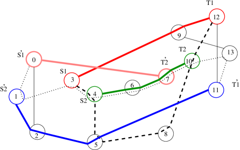
Figure 2: An example of provisioning and protecting four connections on NSFNET.

In the above example, it is assumed that each connection is established at an electronic layer, i.e., an overlay layer above the physical layer. For example, the working path of a connection can be routed and established as an MPLS Label Switched Path (LSP), which can be explicitly routed in the network, as shown in the figure, and therefore the paths of the connections which are jointly protected, e.g., $C_{1}$ and $C_{2}$ in the above example, can be made link disjoint. However, when it comes to the protection path, since the data units transmitted on this path need to be processed, the protection path can be provisioned as segments, where each segment is an MPLS LSP which is explicitly routed. For the example of Figure 2, the protection path protecting connections $C_{1}$ and $C_{2}$ can be provisioned as three MPLS LSPs, namely, (3,4), (4,5,8,10) and (10,12).

III-B Encoding Operations on $\mathbf{S}$ and $\mathbf{T}$

The network encoding operation is executed by each node in ${\cal S}$ and ${\cal T}$. To facilitate the specification of the encoding protocol we first define the following.

• $T(S_{i})$: node in ${\cal T}$ transmitting to and receiving from $S_{i}$, e.g. in Fig.1, $T(S_{1})=T_{2}$.

• $S(T_{j})$: node in ${\cal S}$ transmitting to and receiving from $T_{j}$.

• $\sigma(S_{i})/\sigma(T_{j})$: the next node downstream from $S_{i}$ (respectively $T_{j}$) on $\mathbf{S}$, e.g., in Fig.1, $\sigma(S_{2})=S_{3}$.

• $\sigma^{-1}(S_{i})/\sigma^{-1}(T_{j})$: the next node upstream from $S_{i}$ (respectively $T_{j}$) on $\mathbf{S}$, e.g., in Fig.1, $\sigma^{-1}(T_{5})=S_{4}$.

• $\tau(S_{i})/\tau(T_{j})$: the next node downstream from $S_{i}$ (respectively $T_{j}$) on $\mathbf{T}$, e.g., in Fig. 1, $\tau(T_{4})=S_{5}$.

• $\tau^{-1}(S_{i})/\tau^{-1}(T_{j})$: the next node upstream from $S_{i}$ (respectively $T_{j}$) on $\mathbf{T}$,e.g., in Fig.1, $\tau^{-1}(S_{5})=T_{4}$.

We denote the data unit transmitted on link $e\in\mathbf{S}$ by $y_{e}$ and the data unit transmitted on link $e\in\mathbf{T}$ by $z_{e}$. Assume that nodes $S_{i}$ and $T_{j}$ are in the same connection. The encoding operations work as follows, where all data units belong to the same round.

1. Encoding operations at $S_{i}$. The node $S_{i}$ has access to data units $d_{i}$ (that it generated) and data unit $\hat{u}_{j}$ received on the primary path from $T_{j}$.

   1. It computes $y_{\sigma^{-1}(S_{i})\rightarrow S_{i}}+(d_{i}+\hat{u}_{j})$ and sends it on the link $S_{i}\rightarrow\sigma(S_{i})$; i.e.

      $$y_{S_{i}\rightarrow\sigma(S_{i})} =y_{\sigma^{-1}(S_{i})\rightarrow S_{i}}+(d_{i}+\hat{u}_{j}).$$

   2. It computes $z_{\tau^{-1}(S_{i})\rightarrow S_{i}}+(d_{i}+\hat{u}_{j})$ and sends it on the link $S_{i}\rightarrow\tau(S_{i})$; i.e.

      $$z_{S_{i}\rightarrow\tau(S_{i})} =z_{\tau^{-1}(S_{i})\rightarrow S_{i}}+(d_{i}+\hat{u}_{j}).$$

2. Encoding operations at $T_{j}$. The node $T_{j}$ has access to data units $u_{j}$ (that it generated) and data unit $\hat{d}_{i}$ received on the primary path from $S_{i}$.

   1. It computes $y_{\sigma^{-1}(T_{j})\rightarrow T_{j}}+(\hat{d}_{i}+u_{j})$ and sends it on the link $T_{j}\rightarrow\sigma(T_{j})$; i.e.

      $$y_{T_{j}\rightarrow\sigma(T_{j})} =y_{\sigma^{-1}(T_{j})\rightarrow T_{j}}+(\hat{d}_{i}+u_{j})$$

   2. It computes $z_{\tau^{-1}(T_{j})\rightarrow T_{j}}+(\hat{d}_{i}+u_{j})$ and sends it on the link $T_{j}\rightarrow\tau(T_{j})$; i.e.

      $$z_{T_{j}\rightarrow\tau(T_{j})} =z_{\tau^{-1}(T_{j})\rightarrow T_{j}}+(\hat{d}_{i}+u_{j})$$

An example in which three nodes perform this procedure in the absence of failures is shown in Figure 3.

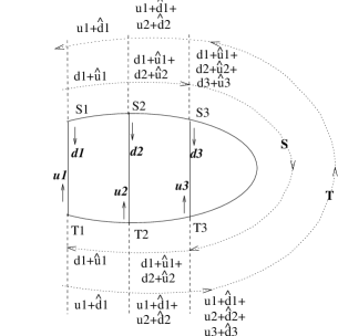
Figure 3: Example of three nodes performing the encoding procedure. Note that the addition (bitwise XOR) of two copies of the same data unit, e.g., $d_{i}$ and $\hat{d}_{i}$, removes both of them.

Consider $S^{\prime}\subseteq{\cal S}$ and let $\mathcal{N}(S^{\prime})$ represent the subset of nodes in ${\cal T}$ that have a primary path connection to the nodes in $S^{\prime}$ (similar notation shall be used for a subset $T^{\prime}\subseteq{\cal T}$). Let $D_{\mathbf{S}}(S_{i})$ and $U_{\mathbf{S}}(S_{i})$ represent the set of downstream and upstream nodes of $S_{i}$ on the protection path $\mathbf{S}$ (similar notation shall be used for the protection path $\mathbf{T}$). When all nodes in ${\cal S}$ and ${\cal T}$ have performed their encoding operations, the signals received at a node $S_{i}$ on the $\mathbf{S}$ and $\mathbf{T}$ paths, respectively, are as follows

$$y_{\sigma^{-1}(S_{i})\rightarrow S_{i}}$$

$$=\underbrace{\sum_{\{k:S_{k}\in U_{\mathbf{S}}(S_{i})\cap{\cal S}\}}d_{k}+\sum_{\{k:T_{k}\in\mathcal{N}(U_{\mathbf{S}}(S_{i})\cap{\cal S})\}}\hat{u}_{k}}_{\text{From nodes upstream of $S_{i}$ on $\mathbf{S}$ in~{}}{\cal S}}$$

$$+\underbrace{\sum_{\{k:T_{k}\in U_{\mathbf{S}}(S_{i})\cap{\cal T}\}}u_{k}+\sum_{\{k:S_{k}\in\mathcal{N}(U_{\mathbf{S}}(S_{i})\cap{\cal T})\}}\hat{d}_{k}}_{\text{From nodes upstream of $S_{i}$ on $\mathbf{S}$ in~{}}{\cal T}},\text{~{}and}$$ (3)

$$z_{\tau^{-1}(S_{i})\rightarrow S_{i}}$$

$$=\underbrace{\sum_{\{k:S_{k}\in U_{\mathbf{T}}(S_{i})\cap{\cal S}\}}d_{k}+\sum_{\{k:T_{k}\in\mathcal{N}(U_{\mathbf{T}}(S_{i})\cap{\cal S})\}}\hat{u}_{k}}_{\text{From nodes upstream of $S_{i}$ on $\mathbf{T}$ in~{}}{\cal S}}$$

$$+\underbrace{\sum_{\{k:T_{k}\in U_{\mathbf{T}}(S_{i})\cap{\cal T}\}}u_{k}+\sum_{\{k:S_{k}\in\mathcal{N}(U_{\mathbf{T}}(S_{i})\cap{\cal T})\}}\hat{d}_{k}}_{\text{From nodes upstream of $S_{i}$ on $\mathbf{T}$ in~{}}{\cal T}}$$ (4)

Similar equations can be derived for node $T_{j}$.

III-C Recovery from failures

The encoding operations described in Subsection III-B allow the recovery of a second copy of the same data unit transmitted on the working circuit, hence protecting against single link failures. To illustrate this, suppose that the primary path between nodes $S_{i}$ and $T_{j}$ fails. In this case, $S_{i}$ does not receive $u_{j}$ on the primary path, and it receives $\hat{u}_{j}=0$ instead. Moreover, $\hat{d}_{i}=0$. However, $S_{i}$ can recover $u_{j}$ by adding equations (3) and (4). In particular node $S_{i}$ computes

$$y_{\sigma^{-1}(S_{i})\rightarrow S_{i}}+z_{\tau^{-1}(S_{i})\rightarrow S_{i}} =\sum_{\{k:S_{k}\in{\cal S}\backslash\{S_{i}\}\}}d_{k}+\sum_{\{k:T_{k}\in{\cal T}\}}u_{k}$$

$$+\sum_{\{k:T_{k}\in{\cal T}\backslash\{T_{j}\}\}}\hat{u}_{k}+\sum_{\{k:S_{k}\in{\cal S}\}}\hat{d}_{k}$$

$$=\hat{d}_{i}+u_{j}$$

$$=u_{j}\text{~{}~{}(since $\hat{d}_{i}=0$.)}$$ (5)

Similarly, $T_{j}$ can recover $d_{i}$ by adding the values it obtains over $\mathbf{S}$ and $\mathbf{T}$ . For example, if the working path between $S_{2}$ and $T_{2}$ in Figure 3 fails, then at node $S_{2}$ adding the signal received on S to the signal received on T, then $u_{2}$ can be recovered, since $T_{2}$ generated $u_{2}$. Also, node $T_{2}$ adds the signals on S and T to recover $d_{2}$.

Notice that the reception of a second copy of $u_{2}$ and $d_{2}$ at $S_{2}$ and $T_{2}$, respectively, when there are no failures, requires the addition of the $d_{2}$ and $u_{2}$ signals generated by the same nodes, respectively.

As a more general example, consider the case in Figure 1. Node $S_{5}$, for example, will receive the following signal on $\mathbf{S}$:

$$(d_{1}+\hat{u}_{2})+(d_{2}+\hat{u}_{5})+(d_{3}+\hat{u}_{1})+(d_{4}+\hat{u}_{4})+(u_{5}+\hat{d}_{2}),$$ (6)

and will receive the following on $\mathbf{T}$:

$$(u_{1}+\hat{d}_{3})+(u_{2}+\hat{d}_{1})+(u_{3}+\hat{d}_{5})+(u_{4}+\hat{d}_{4}).$$ (7)

If the link between $S_{5}$ and $T_{3}$ fails, then $\hat{d}_{5}=0$, and adding equations (6) and (7) will recover $u_{3}$ at $S_{5}$.

IV Implementation Issues

In this subsection we address a number of practical implementation issues.

IV-A Round Numbers

Since linear combinations include packets belonging to the same round number, the packet header should include a round number field. The field is initially reset to zero, and is updated independently by each node when it generates and sends a new packet on the working circuit. Note that there will be a delay before the linear combination propagating on $\mathbf{S}$ and $\mathbf{T}$ reaches a given node. For example, in Figure 3 assuming that all nodes started transmission at time $0$, node $S_{3}$ shall receive the combination corresponding to round $0$ over $\mathbf{S},d_{1}(0)+\hat{u}_{1}(0)+d_{2}(0)+\hat{u}_{2}(0)$ after a delay corresponding to the propagation delay between nodes $S_{1}$ and $S_{3}$, in addition to the processing and transmission times at nodes $S_{1}$ and $S_{2}$. However since the received data unit shall contain the round number $0$, it shall be combined with the data unit generated by $S_{3}$ at time slot $0$.

The size of the round number field depends on the delay of the protection path, including processing and transmission times, as well as propagation time, and the working circuit delay. It is reasonable to assume that the delay of any working circuit is shorter than that of the protection circuit; otherwise, the protection path could have been used as a working path. Thus, when a data unit on the protection path corresponding to a particular round number reaches a given node, the data unit of that round number would have already been received on the primary path of the node.

In this case, it is straightforward to see that once a data unit is transmitted on the working circuit, then it will take no more than twice the delay of the protection path to recover the backup copy of this data unit by the receiver. Therefore, round numbers can then be reused. Based on this argument, the size of the set of required unique round numbers is upper bounded by $2a$, where

$$a=\lceil\frac{\chi_{\bf P}}{(Protection~{}data~{}unit~{}size~{}in~{}bits)/B}\rceil~{}~{}.$$ (8)

$\chi_{\bf P}$ in the above equation is the delay over the protection circuit, and $B$ is the transport capacity of the protection circuit, which, as stated in Section II-B, is taken as the maximum over all the transport capacities of the protected connections. A sufficiently long round number field will require no more than $\log_{2}(2a)$ bits.

IV-B Synchronization

An important issue is node synchronization to rounds. This can be achieved using a number of strategies. A simple strategy for initialization and synchronization is the following:

• In addition to buffers used to store transmitted and received data units, each node $S_{i}\in{\cal S}$ has two buffers, $F_{\bf S}(S_{i})$ and $F_{\bf T}(S_{i})$, which are used for transmissions on the $\mathbf{S}$ and $\mathbf{T}$ paths, respectively. Node $T_{j}\in{\cal T}$ also has similar buffers, $F_{\bf S}(T_{j})$ and $F_{\bf T}(T_{j})$.

• Node $S_{1}$ starts the transmission of $d_{1}(0)$ on the working circuit to $T(S_{1})$. When $S_{1}$ receives $\hat{u}_{T(S_{1})}(0)$, it forms $d_{1}(0)+\hat{u}_{T(S_{1})}(0)$ and transmits it on the outgoing link in $\mathbf{S}$. Similarly, node $T_{1}$ will transmit $u_{1}(0)$ on the working circuit, and $u_{1}(0)+\hat{d}_{S(T_{1})}(0)$ on the outgoing link in $\mathbf{T}$.

• Node $S_{i}$, for $i>0$, will buffer the combinations received on $\mathbf{S}$ in $F_{\bf S}(S_{i})$. Assume that the combination with the smallest round number buffered in $F_{\bf S}(S_{i})$ (i.e., head of buffer) corresponds to round number $n$. When $S_{i}$ transmits $d_{i}(n)$ and receives $\hat{u}_{T(S_{i})}(n)$, then it adds those data units to the combination with the smallest round number in $F_{\bf S}(S_{i})$ and transmits the combination on $\mathbf{S}$. The combination with round number $n$ is then purged from $F_{\bf S}(S_{i})$. Similar operations are performed on $F_{\bf T}(S_{i})$, $F_{\bf S}(T_{j})$ and $F_{\bf T}(T_{j})$. Note that purging of the data unit from the buffer only implies that the combination corresponding to round $n$ has been sent and should not be sent again. However node $S_{i}$ needs to ensure that it saves the value of the data unit received on $\mathbf{S}$ as long as needed for it to be able to decode ${u}_{T(S_{i})}(n)$ if needed. An illustration of the use of those buffers is shown in Figure 4.

  

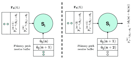
  Figure 4: An illustration of the use of node buffer $F_{\bf S}(S_{i})$. (a) Shows the status of the buffers before data unit at round $n$ has been processed. (b) Shows the status of the buffers after the data unit at round $n$ has been processed. Note that the data units corresponding to round $n$ have been purged from both $F_{\bf S}(S_{i})$ and the primary path receive buffer. The operation of other buffers is similar.

IV-C Buffer Size

Assuming that all nodes start transmitting simultaneously, then all nodes would have decoded the data units corresponding to a given round number in a time that does not exceed

$$\chi_{\bf P}+\max_{1\leq w\leq N}\chi_{w}$$

where $\chi_{w}$ is the delay over working path $w$.

Based on this, the following upper bounds on buffer sizes can be established:

• The transmit buffer, as well as the $F_{\bf S}$ and $F_{\bf T}$ buffers are upper bounded by

  $$\lceil\frac{\chi_{\bf P}+\max_{1\leq w\leq N}\chi_{w}}{Data~{}unit~{}size~{}in~{}bits/B}\rceil~{}~{}.$$

  This is because it will take $\chi_{w}$ units of time over the path $w$ used by the connection $S(T_{1})\leftrightarrow T_{1}$ to receive $\hat{d}_{S(T_{1})}$, and then start transmission on the $\mathbf{T}$ path. An additional $\chi_{P}$ units of time is required for the first combination to reach $S_{1}$. The numerator in the above equation is the maximum of this delay.

• The receive buffer is upper bounded by

  $$\lceil\frac{\chi_{\bf P}+\max_{1\leq w\leq N}\chi_{w}-\min_{1\leq w\leq N}\chi_{w}}{Data~{}unit~{}size~{}in~{}bits/B}\rceil~{}~{}.$$

  The numerator in the above equation is derived using arguments similar to the transmit buffer, except that for the first data unit to be received, it will have to encounter the delay over the working circuit; hence, the subtraction of the minimum such delay.

V Protection against multiple faults

We now consider the situation when protection against multiple (more than one) link failures is required. In this case it is intuitively clear that a given primary path connection needs to be protected by multiple bi-directional protection paths. To see this we first analyze the sum of the signals received on $\mathbf{S}$ and $\mathbf{T}$ for a node $S_{i}$ that has a connection to node $T_{j}$ when the primary paths $S_{i}\leftrightarrow T_{j}$ and $S_{i^{\prime}}\leftrightarrow T_{j^{\prime}}$ protected by the same protection path are in failure. In this case we have $\hat{d}_{i}=\hat{d}_{i^{\prime}}=\hat{u}_{j}=\hat{u}_{j^{\prime}}=0$. Therefore, at node $S_{i}$ we have,

$$y_{\sigma^{-1}(S_{i})\rightarrow S_{i}}+z_{\tau^{-1}(S_{i})\rightarrow S_{i}} =\sum_{\{k:S_{k}\in{\cal S}\backslash\{S_{i}\}\}}d_{k}+\sum_{\{k:T_{k}\in{\cal T}\}}u_{k}$$

$$+\sum_{\{k:T_{k}\in{\cal T}\backslash\{T_{j}\}\}}\hat{u}_{k}+\sum_{\{k:S_{k}\in{\cal S}\}}\hat{d}_{k}$$

$$=(d_{i^{\prime}}+u_{j^{\prime}})+u_{j}.$$

Note that node $S_{i}$ is only interested in the data unit $u_{j}$ but it can only recover the sum of $u_{j}$ and the term $(d_{i^{\prime}}+u_{j^{\prime}})$, in which it is not interested.

We now demonstrate that if a given connection is protected by multiple protection paths, a modification of the protocol presented in Section III-B can enable the nodes to recover from multiple failures. In the modified protocol a node multiplies the sum of its own data unit and the data unit received over its primary path by an appropriately chosen scaling coefficient before adding it to the signals on the protection path. The scheme in Section III-B can be considered to be a special case of this protocol when the scaling coefficient is $1$ (i.e., the identity element over $GF(2^{m})$).

It is important to note that in contrast to the approach presented in [14], this protocol does not require any synchronization between the operation of the different protection paths.

As before, suppose that there are $N$ bi-directional unicast connections that are to be protected against the failure of any $M$ links, for $M\leq N$. These connections are now protected by $K$ protection paths $\mathbf{P}_{k},k=1,\dots,K$. Protection path $\mathbf{P}_{k}$ passes through all nodes ${\cal S}_{k}\subseteq{\cal S}$ and ${\cal T}_{k}\subseteq{\cal T}$ where the nodes in ${\cal S}_{k}$ communicate bi-directionally with the nodes in ${\cal T}_{k}$. Note that $\cup_{k=1}^{K}{\cal S}_{k}={\cal S}$ and $\cup_{k=1}^{K}{\cal T}_{k}={\cal T}$. The ordered sets ${\cal S}_{k}$ and ${\cal S}_{l}$ are not necessarily disjoint for $l\neq k$, i.e., a primary path can be protected by different protection paths. However, if two protection paths are used to protect the same working connection, then they must be link disjoint.

V-A Modified Encoding Operation

Assume that nodes $S_{i}$ and $T_{j}$ are protected by the protection path $\mathbf{P}_{k}$. The encoding operations performed by $S_{i}$ and $T_{j}$ for path $\mathbf{P}_{k}$ are explained below (the operations for other protection paths are similar). In the presentation below we shall use the notation $\sigma(S_{i}),\sigma^{-1}(S_{i}),\tau(S_{i}),\tau^{-1}(S_{i})$ to be defined implicitly over the protection path $\mathbf{P}_{k}$. Similar notation is used for $T_{j}$.

The nodes $S_{i}$ and $T_{j}$ initially agree on a value of the scaling coefficient denoted $\alpha_{i\leftrightarrow j,k}\in GF(2^{m})$. The subscript $i\leftrightarrow j,k$ denotes that the scaling coefficient is used for connection $S_{i}$ to $T_{j}$ over protection path $\mathbf{P}_{k}$.

1. Encoding operations at $S_{i}$. The node $S_{i}$ has access to data units $d_{i}$ (that it generated) and data unit $\hat{u}_{j}$ received on the primary path from $T_{j}$.

   1. It computes $y_{\sigma^{-1}(S_{i})\rightarrow S_{i}}+\alpha_{i\leftrightarrow j,k}(d_{i}+\hat{u}_{j})$ and sends it on the link $S_{i}\rightarrow\sigma(S_{i})$; i.e.

      $$y_{S_{i}\rightarrow\sigma(S_{i})} =y_{\sigma^{-1}(S_{i})\rightarrow S_{i}}+\alpha_{i\leftrightarrow j,k}(d_{i}+\hat{u}_{j}).$$

   2. It computes $z_{\tau^{-1}(S_{i})\rightarrow S_{i}}+\alpha_{i\leftrightarrow j,k}(d_{i}+\hat{u}_{j})$ and sends it on the link $S_{i}\rightarrow\tau(S_{i})$; i.e.

      $$z_{S_{i}\rightarrow\tau(S_{i})} =z_{\tau^{-1}(S_{i})\rightarrow S_{i}}+\alpha_{i\leftrightarrow j,k}(d_{i}+\hat{u}_{j}).$$

2. Encoding operations at $T_{j}$. The node $T_{j}$ has access to data units $u_{j}$ (that it generated) and data unit $\hat{d}_{i}$ received on the primary path from $S_{i}$.

   1. It computes $y_{\sigma^{-1}(T_{j})\rightarrow T_{j}}+\alpha_{i\leftrightarrow j,k}(\hat{d}_{i}+u_{j})$ and sends it on the link $T_{j}\rightarrow\sigma(T_{j})$; i.e.

      $$y_{T_{j}\rightarrow\sigma(T_{j})} =y_{\sigma^{-1}(T_{j})\rightarrow T_{j}}+\alpha_{i\leftrightarrow j,k}(\hat{d}_{i}+u_{j})$$

   2. It computes $z_{\tau^{-1}(T_{j})\rightarrow T_{j}}+\alpha_{i\leftrightarrow j,k}(\hat{d}_{i}+u_{j})$ and sends it on the link $T_{j}\rightarrow\tau(T_{j})$; i.e.

      $$z_{T_{j}\rightarrow\tau(T_{j})} =z_{\tau^{-1}(T_{j})\rightarrow T_{j}}+\alpha_{i\leftrightarrow j,k}(\hat{d}_{i}+u_{j})$$

It should be clear that we can find expressions similar to the ones in (3) and (4) in this case as well.

V-B Recovery from failures

Suppose that the primary paths $S_{i}\leftrightarrow T_{j}$ and $S_{i^{\prime}}\leftrightarrow T_{j^{\prime}}$ fail, and they are both protected by $\mathbf{P}_{k}$. Consider the sum of the signals received by node $S_{i}$ over $\mathbf{S}_{k}$ and $\mathbf{T}_{k}$. Similar to our discussion in III-C, we can observe that

$$y_{\sigma^{-1}(S_{i})\rightarrow S_{i}}+z_{\tau^{-1}(S_{i})\rightarrow S_{i}} =\alpha_{i^{\prime}\leftrightarrow j^{\prime},k}(d_{i^{\prime}}+u_{j^{\prime}})+\alpha_{i\leftrightarrow j,k}u_{j}$$

Note that the structure of the equation allows the node $S_{i}$ to treat $(d_{i^{\prime}}+u_{i^{\prime}})$ as a single unknown. Thus from protection path $\mathbf{P}_{k}$, node $S_{i}$ obtains one equation in two variables. Now, if there exists another protection path $\mathbf{P}_{l}$ that also protects the connections $S_{i}\leftrightarrow T_{j}$ and $S_{i^{\prime}}\leftrightarrow T_{j^{\prime}}$, then we can obtain the following system of equations in two variables

$$\begin{bmatrix}\alpha_{i^{\prime}\leftrightarrow j^{\prime},k}&\alpha_{i\leftrightarrow j,k}\\ \alpha_{i^{\prime}\leftrightarrow j^{\prime},l}&\alpha_{i\leftrightarrow j,l}\end{bmatrix}\begin{bmatrix}(d_{i^{\prime}}+u_{j^{\prime}})\\ u_{j}\end{bmatrix}=\begin{bmatrix}x^{k}_{S_{i}}\\ x^{l}_{S_{i}}\end{bmatrix},$$ (9)

where $x^{k}_{S_{i}}$ and $x^{l}_{S_{i}}$ represent values that can be obtained at $S_{i}$ and therefore $u_{j}$ can be recovered by solving the system of equations. The choice of the scaling coefficients needs to be such that the associated $2\times 2$ matrix in (9) is invertible. This can be guaranteed by a careful assignment of the scaling coefficients. More generally we shall need to ensure that a large number of such matrices need to be full-rank. By choosing the operating field size $GF(2^{m})$ to be large enough, i.e., $m$ to be large enough we can ensure that such an assignment of scaling coefficients always exists [24]. The detailed discussion of coefficient assignment can be found in Section VI.

V-C Conditions for Data Recovery:

We shall first discuss the conditions for data recovery under a certain failure pattern. To facilitate the discussion on determining which failures can be recovered from, we represent the failed connections, and the protection paths using a bipartite graph, $G_{DR}(V,E)$, where the set of vertices $V=\mathbb{N}\cup\mathbb{P}$, and the set of edges $E\subseteq\mathbb{N}\times\mathbb{P}$ where $\mathbb{N}$ is the set of connections to be protected, and $\mathbb{P}$ is the set of protection paths. There is an edge from connection $N_{i}\in\mathbb{N}$ to protection path $\mathbf{P}_{k}\in\mathbb{P}$ if $\mathbf{P}_{k}$ protects connection $N_{i}$. In addition, each edge has a label that is assigned as follows. Suppose that there exists an edge between $N_{i}$ (between nodes $S_{i^{\prime}}$ and $T_{j^{\prime}}$) and $\mathbf{P}_{k}$. The label on the edge is given by the scaling coefficient $\alpha_{i^{\prime}\leftrightarrow j^{\prime},k}$.

Note that in general one could have link failures on primary paths as well as protection paths. Suppose that a failure pattern is specified as a set $F=\{N_{i_{1}},\dots N_{i_{n}}\}\cup\{\mathbf{P}_{j_{1}},\dots,\mathbf{P}_{j_{n^{\prime}}}\}$ where $\{N_{i_{1}},\dots N_{i_{n}}\}$ denotes the set of primary paths that have failed and $\{\mathbf{P}_{j_{1}},\dots,\mathbf{P}_{j_{n^{\prime}}}\}$ denotes the set of protection paths that have failed. The determination of whether a given node can recover from the failures in $F$ can be performed in the following manner.

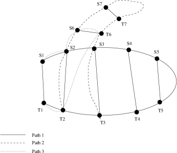
Figure 5: An example of a network protected against multiple faults.

1. Initialization. Form the graph $G_{DR}(V,E)$ as explained above.

2. Edge pruning.

   1. For all connections $N_{i}\in\mathbb{N}\setminus F$ remove $N_{i}$ and all edges in which it participates from $G_{DR}$.

   2. For all protection paths $\mathbf{P}_{i}\in F$ remove $\mathbf{P}_{i}$ and all edges in which it participates from $G_{DR}$.

3. Checking the system of equations. Let the residual graph be denoted $G_{DR}^{{}^{\prime}}=(\mathbb{N}^{{}^{\prime}}\cup\mathbb{P}^{{}^{\prime}},\mathbb{E}^{{}^{\prime}})$. For each connection $N_{i}\in\mathbb{N}^{{}^{\prime}}$, do the following steps.

   1. Let the subset of nodes in $\mathbb{P}^{{}^{\prime}}$ that have a connection to $N_{i}$ be denoted $\mathcal{N}(N_{i})$. Each node in $\mathcal{N}(N_{i})$ corresponds to a linear equation that is available to the nodes participating in $N_{i}$. The linear combination coefficients are determined by the labels of the edges. Identify this system of equations.

   2. Check to see whether a node in $N_{i}$ can solve this system of equations to obtain the data unit it is interested in.

In Figure 6 we show an example that applies to the network in Figure 5. Figure 6.(a) shows the bipartite graph for the entire network, while Figures 6.(b) and 6.(c) show the graph corresponding to the following two failing patterns, respectively:

• ($S_{2},T_{2}$), ($S_{6},T_{6}$) and ($S_{5},T_{5}$)

• $\mathbf{P}_{2}$, ($S_{2},T_{2}$) and ($S_{6},T_{6}$)

Let us assume that the encoding coefficients are chosen to make sure the equation obtained by each node has unique solution. From Figure 6.(b), the failures of connections ($S_{2},T_{2}$) and ($S_{6},T_{6}$) can be recovered from because each node obtains two equations in two unknowns. More specifically, at node $S_{2}$ we obtain the following system of equations (the equation from $\mathbf{P}_{1}$ is not used).

$$\begin{bmatrix}\alpha_{2\leftrightarrow 2,2}&\alpha_{6\leftrightarrow 6,2}\\ \alpha_{2\leftrightarrow 2,3}&\alpha_{6\leftrightarrow 6,3}\end{bmatrix}\begin{bmatrix}u_{2}\\ (d_{6}+u_{6})\end{bmatrix}=\begin{bmatrix}x^{2}_{S_{2}}\\ x^{3}_{S_{2}}\end{bmatrix},$$

which has a unique solution if $(\alpha_{2\leftrightarrow 2,2}\alpha_{6\leftrightarrow 6,3}-\alpha_{2\leftrightarrow 2,3}\alpha_{6\leftrightarrow 6,2})\neq 0$. As pointed out in Section V-B, the choice of the scaling coefficients can be made so that all possible matrices involved have full rank by working over a large enough field size. Thus in this case $S_{2}$ and $T_{2}$ can recover from the failures. By a similar argument we can observe that $S_{6}$ and $T_{6}$ can also recover from the failures by using the equations from $\mathbf{P}_{2}$ and $\mathbf{P}_{3}$. However, $S_{5}$ and $T_{5}$ cannot recover from the failure since they can only obtain one equation from $\mathbf{P}_{1}$ in two variables that corresponds to failures on ($S_{2},T_{2}$) and ($S_{5},T_{5}$). In Figure 6.(c), path $\mathbf{P}_{2}$ does not exist, and ($S_{6}$,$T_{6}$) is protected only by path $\mathbf{P}_{3}$, which protects two failed connections. Therefore, it cannot recover from the failure. However, ($S_{2}$, $T_{2}$) can still recover its data units by using path $\mathbf{P}_{1}$.

In general, this procedure needs to be performed for every possible failure pattern that needs to be protected against, for checking whether all nodes can still recover the data unit that they are interested in. However, usually the set of failure patterns to be protected against is the set of all single link failures or more generally the set of all possible $M\geq 1$ link failures. Those $M$ link failures can happen anywhere, on primary paths or protection paths.

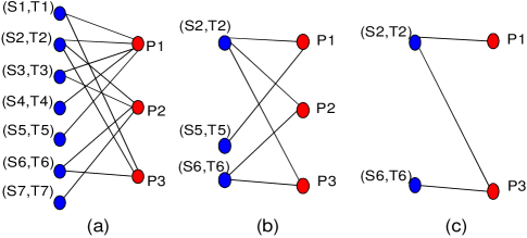
Figure 6: Applying the bipartite graph representation verify if failures will be recovered.

Next, we consider general conditions for data recovery. First, we describe the general model for multiple failures. In order to make expressions simple, we assume that the data unit obtained by a node of a failed connection, say $S_{i}$, from protection path $\mathbf{P}_{k}$ is the sum of the data units from $\mathbf{S}_{k}$, $\mathbf{T}_{k}$. Adding up with $\alpha_{i\leftrightarrow j,k}d_{i}$, which is the data units generated at node $S_{i}$, we denote this sum by $p_{k}$ where $p_{k}=y_{\sigma^{-1}(S_{i})\rightarrow S_{i}}+z_{\tau^{-1}(S_{i})\rightarrow S_{i}}+\alpha_{i\leftrightarrow j,k}d_{i}$. Note that $d_{i}$ is the local data units, which is always available. In this case, each node on one protection path $P_{k}$ obtains the same equation in terms of the same variables. By denoting the set of failed primary connections protected by $\mathbf{P}_{k}$ as $F(\mathbf{P}_{k})$, the equation for this protection path $\mathbf{P}_{k}$ is

$$\sum_{(S_{i}\leftrightarrow T_{j})\in F(\mathbf{P}_{k})}\alpha_{i\leftrightarrow j,k}(d_{i}+u_{j})=p_{k}.$$ (10)

In equation (10), each $d_{i}+u_{j}$ is considered as one variable and the coefficients assigned to $d_{i}$ and $u_{j}$ are the same. Each node of a failed connection will obtain one equation from each intact protection path that protects it and consequently forms a system of linear equations. The number of equations that node $S_{i}$ obtains is the number of intact protection paths that protect $S_{i}$. The number of variables is the total number of failed connections protected by the protection paths that also provide protection to the failed connection between $S_{i}$ and $T_{j}$. $S_{i}$ needs to solve the system of equations and obtain $d_{i}+u_{j}$. By subtracting $d_{i}$, it can get $u_{j}$, which is the data unit $S_{i}$ wants to receive while $T_{j}$ can retrieve the data $d_{i}$ by subtracting $u_{j}$ from $d_{i}+u_{j}$.

Each protection path maps to an equation in terms of a number of variables representing the combination of the data units generated at two end nodes of the failed connections protected by this path. We can form a system of equations that consists of at most $K$ equations like equation (10) where $K$ is the total number of protection paths. Each failure of a primary path introduces a variable whereas each failure occurring on a protection path erases the corresponding equation from the matrix. In general, the system of equations that a node obtains also depends on the topology. If all of the connections are not protected by the same protection paths, there are zeros in the coefficient matrix because a failed connection is not protected by all protection paths, implying that some variables will not appear in all equations.

In order to recover from any failure pattern of $M$ failures, we require the following necessary conditions.

Theorem 1

In order for the network to be guaranteed protection against any $M$ link failures, the following necessary conditions should be satisfied.

1. Each node should be protected by at least $M$ link-disjoint protection paths.

2. Under any failure pattern with $M$ failures, a subset of equations that each node obtains should have a unique solution.

proof: The first condition can be shown by contradiction. If a node is protected by $M-1$ protection paths, the failure could happen on these $M-1$ protection paths and on the primary path in which this node participates. Then, this node does not have any protection path to recover from its primary path failure.

The second condition is to ensure that each node can recover the data unit under any failure pattern with $M$ failures. Note that for necessary condition, we don’t require that the whole system of equations each node obtains has unique solution because one node is only interested in recovering the data unit sent to it. As long as it can solve a subset of the equations, it recovers from its failure.  $\blacksquare$We emphasize that the structure of the equations depends heavily on the network topology, the connections provisioned and the protection paths. Therefore it is hard to state a more specific result about the conditions under which protection is guaranteed. However, under certain structured topologies it may be possible to provide a characterization of the conditions that can be checked without having to verify each possible system of equations.

For example, if all connections are protected by $M$ protection paths, it is easy to see the sufficient condition for data recovery from any $M$ failures is that the coefficient matrix of the system of equations each node obtains under any failure pattern with $M$ failures has full rank. As will be shown next, our coefficient assignment methods are such that the sufficient conditions above hold.

Next we construct a $K\times N$ matrix to facilitate the discussion of coefficient assignment. According to the encoding protocol, each connection $S_{i}-T_{j}$ has coefficient $\alpha_{i\leftrightarrow j,k}$ for encoding on $\mathbf{P}_{k}$. In general, there are at most $K\times N$ coefficients for a network with $N$ primary paths $S_{i_{1}}\leftrightarrow T_{j_{1}},S_{i_{2}}\leftrightarrow T_{j_{2}},\ldots,S_{i_{l}}\leftrightarrow T_{j_{l}},\ldots,S_{i_{N}}\leftrightarrow T_{j_{N}}$ and $K$ protection paths $\mathbf{P}_{1},\mathbf{P}_{2},\ldots,\mathbf{P}_{K}$. We form a $K\times N$ matrix $\cal A$ where ${\cal A}_{kl}=\alpha_{i_{l}\leftrightarrow j_{l},k}$ if $S_{i_{l}}\leftrightarrow T_{i_{l}}$ is protected by $\mathbf{P}_{k}$, ${\cal A}_{kl}=0$ otherwise. Here, $l$ is the index for primary paths and each column of $\cal A$ corresponds to a primary path. Each row of $\cal A$ corresponds to a protection path. This matrix contains all encoding coefficients and some zeros induced by the topology in general. It is easy to see that under any failure pattern, the coefficient matrix of the system of equations at any node of any failed connection is a submatrix of matrix ${\cal A}$. We require these submatrices of ${\cal A}$ to have full rank. We shall discuss the construction of ${\cal A}$, i.e., assign proper coefficients in Section VI.

VI Encoding coefficient assignment

In this section, we shall discuss encoding coefficient assignment strategies for the proposed network coding schemes, i.e., construct ${\cal A}$ properly. Under certain assumptions on the topology, two special matrix based assignments can provide tight field size bound and efficient decoding algorithms. We shall also introduce matrix completion method for general topologies.

Note that the coefficient assignment is done before the actual transmission. Once the coefficients have been determined, during data transmission they need not be changed. Thus, for the schemes that guarantee successful recovery with high probability, we can keep generating the matrix ${\cal A}$ until the full rank condition discussed at the end of the previous section satisfies. This only needs to be done once. After that, during the actual transmission, the recovery is successful for sure.

VI-A Special matrix based assignment

In this and the next subsection, we assume that all primary paths are protected by the same protection paths. This implies that matrix $\cal A$ only consists of encoding coefficients. It does not contain zeros induced by the topology. Thus, we can let $\cal A$ to be a matrix with some special structures such that any submatrix of $\cal A$ has full rank. The network will be able to recover from any failure pattern with $M$ (or less) failures. Without loss of generality, we shall focus on the case when $M=K$, where $K$ is the number of protection paths. If $M$ failures happen, in which $t_{1}$ failures happen on primary paths, each node will get $M-(M-t_{1})=t_{1}$ equations with $t_{1}$ unknowns corresponding to $t_{1}$ primary path failures. The $t_{1}\times t_{1}$ coefficient matrix is a square submatrix of $\cal A$ and they are the same for each node under one failure pattern.

First, we shall show a Vandermonde matrix-based coefficient assignment. It requires the field size to be $q\geq N$. If all failures happen on primary paths, the recovery at each node is guaranteed. In this assignment strategy, we pick up $N$ distinct elements from $GF(q)$: $\lambda_{1},\ldots,\lambda_{N}$ and assign them to each primary paths. At nodes $S_{i_{l}}$ and $T_{j_{l}}$, $\lambda_{l}^{k-1}$ is used as encoding coefficient on protection path $\mathbf{P}_{k}$, i.e., ${\cal A}_{kl}=\alpha_{i_{l}\leftrightarrow j_{l},k}=\lambda_{l}^{k-1}$. In other words, $\cal A$ is a Vandermonde matrix [26, Section 6.1]:

$$\left[\begin{array}[]{cccc}1&1&\cdots&1\\ \lambda_{1}&\lambda_{2}&\cdots&\lambda_{N}\\ \lambda_{1}^{2}&\lambda_{2}^{2}&\cdots&\lambda_{N}^{2}\\ \cdots&\cdots&\cdots&\cdots\\ \lambda_{1}^{K-1}&\lambda_{2}^{K-1}&\cdots&\lambda_{N}^{K-1}\end{array}\right].$$

Suppose $M$ failures happen on primary paths, the indices of failed connections are $e_{1},\ldots,e_{M}$, every node gets a system of linear equations with coefficient matrix having this form:

$$\left[\begin{array}[]{cccc}1&1&\cdots&1\\ \lambda_{e_{1}}&\lambda_{e_{2}}&\cdots&\lambda_{e_{M}}\\ \lambda_{e_{1}}^{2}&\lambda_{e_{2}}^{2}&\cdots&\lambda_{e_{M}}^{2}\\ \cdots&\cdots&\cdots&\cdots\\ \lambda_{e_{1}}^{M-1}&\lambda_{e_{2}}^{M-1}&\cdots&\lambda_{e_{M}}^{M-1}\end{array}\right].$$

This matrix is a $M\times M$ Vandermonde matrix. As long as $\lambda_{e_{1}},\lambda_{e_{2}},\ldots,\lambda_{e_{M}}$ are distinct, this matrix is invertible and $S_{i_{e_{1}}}$ can recover $u_{j_{e_{1}}}$. We choose $\lambda_{1},\ldots,\lambda_{N}$ to be distinct so that the submatrix formed by any $M$ columns of $\cal A$ has full rank. The smallest field size we need is the number of connections we want to protect, i.e., $q\geq N$. Moreover, the complexity of solving linear equation with Vandermonde coefficient matrix is $O(M^{2})$[19]. Thus, we have a more efficient decoding because if the coefficients are arbitrarily chosen, even if it is solvable, the complexity of Gaussian elimination is $O(M^{3})$.

If $M-t_{1}$ failures happen on protection paths, we require that any $t_{1}\times t_{1}$ square submatrix formed by choosing any $t_{1}$ columns and $t_{1}$ rows from $\cal A$ has full rank. Although the chance is large, the Vandermonde matrix can not guarantee this for sure [20, p.323,problem 7],[22],[23]. We shall propose another special matrix to guarantee that for combined failures, the recovery is successful at the expense of a slightly larger field size compared to Vandermonde matrix assignment.

In order to achieve this goal, we resort to Cauchy matrix [20], of which any square submatrix has full rank if the entries are chosen carefully.

Definition 2

Let $\{x_{1},\ldots,x_{m_{1}}\},\{y_{1},\ldots,y_{m_{2}}\}$ be two sets of elements in a field $F$ such that

• $x_{i}+y_{j}\neq 0,\text{~{} }\forall i\in\{1,\ldots,m_{1}\}\text{~{} }\forall j\in\{1,\ldots,m_{2}\}$;

• $\forall i,j\in\{1,\ldots,m_{1}\},i\neq j:x_{i}\neq x_{j}$ and $\forall i,j\in\{1,\ldots,m_{2}\},i\neq j:y_{i}\neq y_{j}$.

The matrix $C=(c_{ij})$ where $c_{ij}=1/(x_{i}+y_{j})$ is called a Cauchy matrix.

If $m_{1}=m_{2}$, the Cauchy matrix becomes square and its determinant is [20]:

$$\det(C)=\frac{\prod_{1\leq i<j\leq m_{1}}(x_{j}-x_{i})(y_{j}-y_{i})}{\prod_{1\leq i,j\leq m_{1}}(x_{i}+y_{j})}$$

Note that in $GF(q)$ where $q$ is some power of $2$, the addition and subtraction are equivalent. Therefore, as long as $x_{1},\ldots,x_{m_{1}},y_{1},\ldots,y_{m_{1}}$ are distinct, Cauchy matrix has full rank and its any square submatrix is also a Cauchy matrix (by definition) with full rank. For our protection problem, we let matrix $\cal A$ to be a $K\times N$ Cauchy matrix. $\{x_{1},\ldots,x_{K}\},\{y_{1},\ldots,y_{N}\}$ are chosen to be distinct. Thus, the smallest field size we need is $K+N$. Suppose there are $t_{1}$ failures on primary paths and $M-t_{1}$ failures on protection paths, the coefficient matrix of the system of equations obtained by a node is a $t_{1}\times t_{1}$ submatrix of $\cal A$. It is still a Cauchy matrix by definition and invertible. Thus, the network can be recovered from any $M$ failures. Moreover, the inversion can be done in $O(t_{1}^{2})$ [21], which provides an efficient decoding algorithm.

VI-B Random assignment

We could also choose the coefficients from a large finite field. More specifically, we have the following claim [27].

Claim 3

When all coefficients are randomly, independently and uniformly chosen from $GF(q)$, the probability that a $t_{1}$-by-$t_{1}$ matrix has full rank is $p(t_{1})=\Pi_{i=1}^{t_{1}}(1-1/q^{i})$, $1\leq t_{1}\leq M$.

Under one failure pattern with $t_{1}$ failures on the primary paths and $M-t_{1}$ failures on the protection paths, every failed connection obtains the equations that have the same $t_{1}$-by-$t_{1}$ coefficient matrix. The probability that it is full rank is $p(t_{1})$ and it goes to 1 when $q$ is large. Note that there are $\sum_{t_{1}=1}^{M}{N\choose t_{1}}{M\choose{M-t_{1}}}$ possible failure patterns when the total number of failures is $M$. Thus, by union bound, the probability of successful recovery under any failure pattern with $M$ failures is $1-\sum_{t_{1}=1}^{M}{N\choose t_{1}}{M\choose{M-t_{1}}}(1-p(t_{1}))$, and it approaches 1 as $q$ increases.

VI-C Matrix completion for general topology

If the primary paths are protected by different protection paths, like in Figure 5, there are some zeros in $\cal A$ induced by the topology. We want to choose encoding coefficients so that under every failure pattern with $M$ or less failures, the coefficient matrix of the system of equations obtained by every node is invertible. We can view the encoding coefficients in $\cal A$ as indeterminates to be decided. The matrices we require to have full rank are a collection ${\cal C}_{\cal A}$ of submatrices of $\cal A$, where ${\cal C}_{\cal A}$ depends on the failure patterns and the network topology. Each matrix in ${\cal C}_{\cal A}$ consists of some indeterminates and some zeros. The problem of choosing encoding coefficients can be solved by matrix completion [24]. A simultaneous max-rank completion of ${\cal C}_{\cal A}$ is an assignment of values from $GF(q)$ to the indeterminates that preserves the rank of all matrices in ${\cal C}_{\cal A}$. After completion, each matrix will have the maximum possible rank. Matrix completion can be done by deterministic algorithms [24]. Moreover, simply choosing a completion at random from a sufficiently large field can achieve the maximum rank with high probability [25]. Hence, we can choose encoding coefficients randomly from a large field.

VII ILP Formulation for Single-link Failure

The problem of provisioning the working paths and their protection paths in a random graph is a hard problem. This is due to the fact that the problem of finding link disjoint paths between multiple pairs of nodes in a graph is known to be NP-complete [17]. Therefore, in this section we formulate an integer linear program that optimally provisions a set of unicast connections, and their protection paths against single-link failure. The optimality criterion is the minimization of the sum of the working and protection resources.

The problem can be stated as follows: Given an bidirectional graph $G=(V,E)$ and a traffic demand matrix of unicast connections, $\mathbb{N}$, establish a connection for each bidirectional traffic request $j\in\mathbb{N}$, and a number of protection paths that travel all the end nodes of the connections in $\mathbb{N}$, defined by set $\mathbb{C}$, such that:

• A path protecting a connection must pass through the end nodes of the connection.

• The connections jointly protected by the same path must be mutually link disjoint, and also link disjoint from the protection path.

• The total number of edges used for both working and protection paths is minimum.

We also assume that the network is uncapacitated.

In order to formulate this problem, we modify the graph $G$ to obtain the graph $G^{\prime}$ by adding a hypothetical source $s$ and a hypothetical sink $t$. We also add a directed edge from $s$ to each node $v$, where $v\in\mathbb{C}$, as well as a directed edge from each such node $v$ to $t$. An example is shown in Figure 7. Figure 7.(a) shows a graph $G$ with six nodes and ten bidirectional edges and the corresponding modification to the graph $G^{\prime}$ given two traffic requests $\mathbb{N}=\{(0,3),(5,2)\}$. Figure 7.(b) shows the provisioning of the two connections in $\mathbb{N}$ and their protection path from $s$ to $t$. Therefore, the problem of finding the protection paths turns out to be establishing connections from node $s$ to $t$ that traverse all the nodes $v\in\mathbb{C}$. For each subset of connections that are protected together, the two ends nodes of these traffic requests have to be traversed by the same protection path.

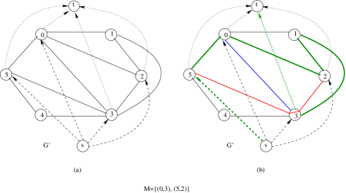
Figure 7: An example to show: (a) the graph $G$ in solid line and its modified graph $G^{\prime}$; (b) the provisioning of the connections ((0-3) and (5-3-2)) and their protection path (s-5-0-2-1-3-t), where the two links (s-5) and (3-t) are not included in the cost of the protection circuit.

This disjoint paths routing problem can be formulated with ILP as follow: (Note that $G=(V,E)$ and $G^{\prime}=(V^{\prime},E^{\prime})$ denote the original and modified graph in the formulation). It is to be noted that the number of protection paths must satisfy:

$$1\leq\mathrm{number~{}of~{}protection~{}paths}\leq N.$$

We may have more than one protection path because it is possible that the primary connections are partitioned into several sets and each set of primary connections share the protection of path. However, the worst case is that each primary path requires a unique protection path (the case of 1+1 protection), which results in a total of $N$ protection paths. In the formulation, therefore, we have a maximum of $2N$ paths:

• Connections indexed from 1 to $N$ are the ones given by the set $\mathbb{N}$, and these should be provisioned in the network.

• Connections indexed from $N{+}1$ to $2N$ are hypothetical connections, which correspond to protection connections, and at least one of them should be provisioned.

The ILP is formulated as a network flow problem, where there is a flow of one unit between each pair of end nodes of a connection, and there is also a flow of one unit from $s$ to $t$ for each protection path.

We define the following parameters, which are input to the ILP:

$G(V,E)$:	the original network graph
$G^{\prime}(V^{\prime},E^{\prime})$:	the modified graph
$\mathbb{N}$:	the set of unicast connections
$c_{mn}$:	a constant, the cost of link $(m,n)\in E$
$v_{j}$:	set of end nodes of connection $j$ in $\mathbb{N}$, $v_{j}=\{s_{j},t_{j}\}$, which are different notations from the previous definition of a connection, denoted by $S_{i}$, $T_{j}$ where $i,j$ are the indices for the nodes.

We also define the following binary variables which are computed by the ILP:

$f^{i}_{mn}$	binary, equals 1 if the protection path $i$ traverses link $(m,n)$ in $G$
$Zf^{i}_{m}$	integer, the number of times that the node $m\in V$ is traversed by path $i$
$U^{i}_{j}$	binary, equals 1 if connection $j$ is protected by path $i$
$p^{j}_{mn}$	binary, equals 1 if the working flow of $j$ traverses link $(m,n)\in G$
$q^{j}_{mn}$	binary, equals 1 if the protection flow of $j$ traverses link $(m,n)\in G$
$Zp^{j}_{m}$	integer, the number of times that node $m\in V$ is traversed by the working flow of $j$
$Zq^{j}_{m}$	integer, the number of times that node $m\in V$ is traversed by the protection flow of $j$

The objective function is:

$$\text{Minimize:}~{}~{}~{}\sum_{(m,n)\in E}(\sum_{1\leq j\leq N}{p^{j}_{mn}c_{mn}}+\sum_{N<i\leq 2N}{f^{i}_{mn}c_{mn}})$$

The objective function minimizes the total cost of links used by the working paths (first term) and by the protection paths (second term). Note that a protection path at $s$ and end at $t$ in the modified graph, $G^{\prime}$, but we only consider the cost of links in the original graph $G$.

The constraints are such that:

1. Working Flow Conservation:

   $$\sum_{\{n:(s_{j},n)\in E\}}{p^{j}_{s_{j}n}}=1,~{}~{}j\leq N;$$ (11)

   $$\sum_{\{n:(m,n)\in E\}}{p^{j}_{mn}=2Zp^{j}_{m}},~{}\forall m\in V{\setminus}c_{j}.$$ (12)

   The constraints (11) and (12) are standard flow conservation for working traffic which ensures that a bidirectional path is established between end nodes $s_{j}$ and $t_{j}$ of connection $j$.

2. Protection Flow Conservation:

   $$\textrm{For }\forall j\leq N,~{}N<i\leq 2N:$$

   $$\sum_{\{n:(s_{j},n)\in E\}}{q^{j}_{s_{j}n}}=1;$$ (13)

   $$\sum_{\{n:(m,n)\in E\}}{q^{j}_{mn}=2Zq^{j}_{m}},~{}\forall m\in V{\setminus}v_{j};$$ (14)

   Constraints (13) and (14) make sure that each connection $j$ has a protection flow.

   $$\sum_{\{n:(s,n)\in E^{\prime}\}}{f^{i}_{sn}}\leq 1;$$ (15)

   $$\sum_{\{n:(m,n)\in E\}}{f^{i}_{mn}=2Zf^{i}_{m}},~{}\forall m\in V;$$ (16)

   The flow conservation of protection paths is ensured by constraints (15) and (16). It is worth noting that not every protection path $i$ $(N{<}i{\leq}2N)$ is required unless it is used for protection.

   $$\sum_{N<i\leq 2N}{U^{i}_{j}}=1;$$ (17)

   $$\frac{1}{N}\sum_{j\leq N}{U^{i}_{j}}\leq\sum_{\{n:(s,n)\in E^{\prime}\}}{f^{i}_{sn}};$$ (18)

   $$f^{i}_{mn}\geq q^{j}_{mn}+U^{i}_{j}-1,~{}\forall(m,n)\in E;$$ (19)

   Each working flow should be protected by exactly one protection path, guaranteed by constraint (17). Meanwhile, any protection path $i$ is provisioned only if it is used to protect any working path $j$. Otherwise, we do not need to provision it. Therefore, equation (18) ensures this constraint. Furthermore, constraint (19) ensures that if a protection path $i$ protects connection $j$, it should traverse the same links used by the protection flow $q^{j}_{mn}$.

3. Protection Path Sharing:

   $$\textrm{For }\forall(m,n)\in E,~{}N<i\leq 2N:$$

   $$p^{j}_{mn}+q^{j}_{mn}\leq 1,~{}~{}~{}\forall j\leq N;$$ (20)

   $$p^{j}_{mn}+f^{i}_{mn}+U^{i}_{j}\leq 2,~{}~{}\forall j\leq N;$$ (21)

   $$p^{j}_{mn}+p^{k}_{mn}+U^{i}_{j}+U^{i}_{k}\leq 3,~{}\forall j<k\leq N.$$ (22)

   The working flow and protection flow of each connection $j$ should be link disjoint, reflected by constraint (20). Each protection path may protect multiple connections so that it needs to traverse multiple corresponding protection flows. Thus, each protection path should also be link disjoint to all the working flow it protects. This constraint is ensured by equation (21). Meanwhile, if two connections are protected by the same path $f$, their working flow should also be link disjoint such that codewords can be decodes at each end nodes through the protection path. The last constraint is guaranteed by equation (22).

The total number of variables used in the ILP is $(3N|V|+3N|E|+N^{2})$ and the total number of constraints is $(6N|V|+2N+2N^{2}|E|+N|E|+N^{2}(N-1)|E|)$, which is dominated by $O(N^{3}|E|)$.

VIII Numerical Results

This section presents numerical results of the cost of our proposed protection scheme and compares it to 1+1 protection and Shared Backup Path Protection (SBPP) in terms of total resource requirements for protection against single-link failure. SBPP has been proven to be the most capacity efficient protection scheme and can achieve optimal solutions [12]. However, it is also a reactive protection mechanism and takes time to detect, localize and recover from failures. We consider two realistic network topologies, NSFNET and COST239, as shown in Fig. 8 and 9, respectively. Both networks are bidirectional and each bidirectional span $e$ has a cost $c_{e}$, which equals the actual distance in kilometers between two end nodes.

We first compare three schemes in terms of the total connection and protection provisioning cost in both networks as shown in Fig. 10 and 11, respectively. We obtained the results by formulating the problems as ILPs using three different approaches. The x-axis denotes the number of connections in the static traffic matrix and y-axis denotes the total network design cost. Each value is the average cost over ten independent cases and all approaches used identical traffic requests for each case.

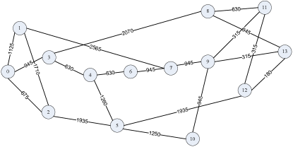
Figure 8: NSFNET (N=14, E=21)

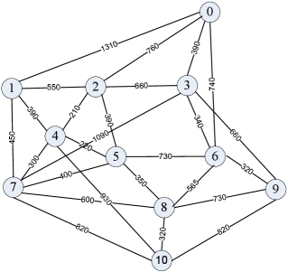
Figure 9: COST239 (N=11, E=26)

Figure 10: Comparison of total cost in NSFNET

Figure 11: Comparison of total cost in COST239 network

Since SBPP is the most capacity efficient scheme, it achieves the minimum cost. 1+N approach uses much lower cost than 1+1, but is higher than SBPP in both networks. We express the extra cost ratio of a scheme over SBPP by: $(Cost_{scheme}-Cost_{SBPP})/Cost_{SBPP}$. The extra cost ratio of 1+N in NSFNET increases from 5.2% to 23% as the number of connections increases from 2 to 7. Meanwhile, the extra cost ratio of 1+1 over SBPP increases from 12% to 45%, which is almost twice that of 1+N at each case. The advantage of 1+N over 1+1 in COST239 is even more significant than NSFNET due to the larger average nodal degree, 4.6, compared to, 3, in NSFNET. Hence, there is a higher chance for multiple primary paths to share the same protection path, which results in lower overall cost. Based on the results, we can observe that the extra cost ratio of 1+N over SBPP in COST239 increases from 1.8% to 11.1% whereas the ratio of 1+1 over SBPP increases from 10.2% to 38%, as the number of connections increases from 2 to 7. Actually, the cost of using 1+N is very close to the optimal in COST239 network. The extra cost required by 1+N over the optimal solution is less than 27% of that achieved by 1+1 scheme.

In fact, if we only consider the cost of protection, i.e. exclude the cost of connection provisioning, 1+N protection uses much lower resources than 1+1 protection. For example, by examining one network scenario where there are seven connections in COST239 network, the average protection cost of using SBPP, 1+N and 1+1 protection schemes is 3586.0, 4313.5 and 6441.5, respectively. The saving ratio of 1+N to 1+1 is around 33%, which is higher than the saving ratio of joint capacity cost (19.3%). This example further illustrates the cost saving advantages of using 1+N protection over 1+1 protection.

In summary, 1+N protection has a traffic recovery speed which is comparable 1+1 protection. However, it performs significantly better than 1+1 scheme in terms of protection cost. Compared with the most capacity efficient protection scheme, SBPP, 1+N protection performs close to SBPP in terms of total capacity cost in dense networks. However, SBPP takes much longer to recover from failures due to the long switch reconfiguration time and traffic rerouting, which are not required in 1+N protection.

IX Conclusions

This paper has introduced a resource efficient, and a fast method for providing protection for a group of connections such that a second copy of each data unit transmitted on the working circuits can be recovered without the detection of the failure, or rerouting data. This is done by linearly combining the data units using the technique of network coding, and transmitting these combinations on a shared set of protection circuits in two opposite directions. The reduced number of resources is due to the sharing of the protection circuit to transmit linear combinations of data units from multiple sources. The coding is the key to the instantaneous recovery of the information. This provides protection against any single link failure on any of the working circuits. The paper also generalized this technique to provide protection against multiple link failures.

The method introduced in this paper improves the technique introduced in [15] and [14]. In particular, (a) it requires fewer protection resources, and (b) it implements coding using a simpler synchronization strategy. A cost comparison study of providing protection against single link failures has shown that the proposed technique introduces a significant saving over typical protection schemes, such as 1+1 protection, while achieving a comparable speed of recovery. The numerical results also show that the cost of our 1+N scheme is close to SBPP, the most capacity efficient protection scheme. However, the proposed scheme in our paper provides much faster recovery than SBPP.

Ahmed E. Kamal Ahmed E. Kamal (S’82-M’87-SM’91)is a professor of Electrical and Computer Engineering at Iowa State University. His research interests include high-performance networks, optical networks, wireless and sensor networks and performance evaluation. He is a senior member of the IEEE, a senior member of the Association of Computing Machinery, and a registered professional engineer. He was the co-recipient of the 1993 IEE Hartree Premium for papers published in Computers and Control in IEE Proceedings for his paper entitled Study of the Behaviour of Hubnet, and the best paper award of the IEEE Globecom 2008 Symposium on Ad Hoc and Sensors Networks Symposium. He served on the technical program committees of numerous conferences and workshops, was the organizer and co-chair of the first and second Workshops on Traffic Grooming 2004 and 2005, respectively, and was the chair of co-chair of the Technical Program Committees of a number of conferences including the Communications Services Research (CNSR) conference 2006, the Optical Symposium of Broadnets 2006, and the Optical Networks and Systems Symposium of the IEEE Globecom 2007, the 2008 ACS/IEEE International Conference on Computer Systems and Applications (AICCSA-08), and the ACM International Conference on Information Science, Technology and Applications, 2009. He is also the Technical Program co-chair of the Optical Networks and Systems Symposium of the IEEE Globecom 2010. He is on the editorial boards of the Computer Networks journal, and the Journal of Communications.

Aditya Ramamoorthy Aditya Ramamoorthy received his B. Tech degree in Electrical Engineering from the Indian Institute of Technology, Delhi in 1999 and the M.S. and Ph.D. degrees from the University of California, Los Angeles (UCLA) in 2002 and 2005 respectively. He was a systems engineer at Biomorphic VLSI Inc. till 2001. From 2005 to 2006 he was with the data storage signal processing group at Marvell Semiconductor Inc. Since Fall 2006 he has been an assistant professor in the ECE department at Iowa State University. He has interned at Microsoft Research in summer 2004 and has visited the ECE department at Georgia Tech, Atlanta in Spring 2005. His research interests are in the areas of network information theory and channel coding.

Long Long Long Long received his B.Eng degree in Electronic Information Engineering from Huazhong University of Science and Technology, Wuhan, China in 2002 and M.Sc degree in Software Engineering from Peking University, Beijing, China in 2005. Since fall 2006, he has been a Ph.D student in ECE department of Iowa State University, USA. His research interests are in the area of traffic grooming and survivability of optical networks.

Shizheng Li Shizheng Li received his B.Eng degree in information engineering from Southeast University (Chien-Shiung Wu Honors College), Nanjing, China, in 2007. He worked on error correction codes in National Mobile Communications Laboratory at Southeast University during 2006 and 2007. Since Fall 2007, he has been a Ph.D. student in the Department of Electrical and Computer Engineering, Iowa State University. His research interests include network coding, distributed source coding and network resource allocation. He received Microsoft Young Fellowship from Microsoft Research Asia in 2006. He is a student member of IEEE.

References

- [1] D. Zhou and S. Subramaniam, “Survivability in optical networks,” IEEE Network, vol. 14, pp. 16–23, Nov./Dec. 2000.
- [2] S. Li and A. Ramamoorthy, “Protection against link errors and failures using network coding,”IEEE Transactions on Communications, to appear. Available: http://arxiv.org/abs/0905.2248
- [3] D. Stamatelakis and W. D. Grover, “Ip layer restoration and network planning based on virtual protection cycles,” IEEE Journal on Selected Areas in Communications, vol. 18, no. 10, pp. 1938–1949, 2000.
- [4] W. D. Grover, Mesh-based survivable networks : options and strategies for optical, MPLS, SONET, and ATM Networking. Upper Saddle River, NJ: Prentice-Hall, 2004.
- [5] C. Fragouli, J.-Y. LeBoudec, and J. Widmer, “Network coding: An instant primer,” ACM Computer Communication Review, vol. 36, pp. 63–68, Jan. 2006.
- [6] D. Schupke and R. Prinz, “Performance of path protection and rerouting for wdm networks subject to dual failures,” in Optical Fiber Conference, pp. 209–210, 2003.
- [7] S. Kim and S. Lumetta, “Evaluation of protection reconfiguration for multiple failures in WDM mesh networks,” in Optical Fiber Conference, pp. 210–211, 2003.
- [8] J. Zhang, K. Zhu, and B. Mukherjee, “Backup provisioning to remedy the effect of multiple link failures in wdm mesh networks,” IEEE Journal on Selected Areas in Communications, vol. 24, pp. 57–67, Aug. 2006.
- [9] H. Choi, S. Subramaniam, and H.-A. Choi, “Loopback recovery from double-link failures in optical mesh networks,” IEEE/ACM Transactions on Networking, vol. 12, pp. 1119–1130, Dec. 2004.
- [10] W. He, M. Sridharan, and A. K. Somani, “Capacity optimization for surviving double-link failures in mesh-restorable optical networks,” Photonic Network Communications, vol. 9, pp. 99–111, Jan. 2005.
- [11] Y. Liu, D. Tipper, and P. Siripongwutikorn, “Approximating optimal spare capacity allocation by successive survivable routing,” IEEE/ACM Transactions on Networking, vol. 13, pp. 198–211, Feb. 2003.
- [12] S. Ramamurthy and B. Mukherjee, “Survivable WDM mesh networks. part I-protection,” in Proceedings of IEEE INFOCOM, 1999.
- [13] A. E. Kamal, “1+N protection in optical mesh networks using network coding on p-cycles,” in the proceedings of the IEEE Globecom, 2006.
- [14] A. E. Kamal, “1+N protection against multiple faults in mesh networks,” in the proceedings of the IEEE International Conference on Communications (ICC), 2007.
- [15] A. E. Kamal, “1+N Network Protection for Mesh Networks: Network Coding-Based Protection using p-Cycles,” IEEE/ACM Transactions on Networking, Vol. 18, No. 1, Feb. 2010, pp. 67–80.
- [16] R. Ahlswede, N. Cai, S.-Y. R. Li, and R. W. Yeung, “Network information flow,” IEEE Transactions on Information Theory, vol. 46, pp. 1204–1216, July 2000.
- [17] J. Vygen, ”NP-completeness of some edge-disjoint paths problems”, Discrete Appl. Math., vol. 46, pp. 83–90, 1995.
- [18] R. Bhandari, Survivable Networks: Algorithms for Diverse Routing. Springer, 1999.
- [19] W. H. Press, B. P. Flannery, S. A. Teukolsky, and W. T. Vetterling, Numerical Recipes in C: The Art of Scientific Computing, 2nd ed. Cambridge University Press, 1992.
- [20] F. J. MacWilliams and N. J. A. Sloane, The Theory of Error-Correcting Codes. North Holland, 1977.
- [21] J. Blomer, M. Kalfane, R. Karp, M. Karpinski, M. Luby, and D. Zuckerman, “An xor-based erasure-resilient coding scheme,” Int. Comput. Sci. Inst., Berkeley, CA, TR-95-048, 1995. [Online]. Available: citeseer.ist.psu.edu/blomer95xorbased.html
- [22] J.Lacan and J.Fimes, “Systematic MDS erasure codes based on Vandermonde matrices,” IEEE Communications Letters, vol. 8, no.9, Sep.2004.
- [23] I. E. Shparlinski, “On singularity of generalized Vandermonde matrices over finite fields”, Finite Fields and Their Applications, vol. 11, no. 2, pp. 193-199, 2005.
- [24] N. J. A. Harvey, D. R. Karger, and K. Murota, “Deterministic network coding by matrix completion,” in SODA ’05: Proceedings of the sixteenth annual ACM-SIAM symposium on Discrete algorithms, 2005, pp. 489–498.
- [25] L.Lovasz, “On determinants, matchings and random algorithms,” in Fund. Comput. Theory 79, Berlin, 1979.
- [26] S. Lin and D. J. Costello, Error control coding: fundamentals and applications. Prentice Hall, 2004.
- [27] C. Cooper, “On the distribution of rank of a random matrix over a finite field,” in Random Struct. Algorithms, vol. 17, no. 3-4, pp.197–212, 2000.