PADDLE: Proximal Algorithm for Dual Dictionaries LEarning

Abstract

Recently, considerable research efforts have been devoted to the design of methods to learn from data overcomplete dictionaries for sparse coding. However, learned dictionaries require the solution of an optimization problem for coding new data. In order to overcome this drawback, we propose an algorithm aimed at learning both a dictionary and its dual: a linear mapping directly performing the coding. By leveraging on proximal methods, our algorithm jointly minimizes the reconstruction error of the dictionary and the coding error of its dual; the sparsity of the representation is induced by an $\ell_{1}$-based penalty on its coefficients. The results obtained on synthetic data and real images show that the algorithm is capable of recovering the expected dictionaries. Furthermore, on a benchmark dataset, we show that the image features obtained from the dual matrix yield state-of-the-art classification performance while being much less computational intensive.

1 Introduction

The representation of a signal as the superposition of elementary signals, or atoms, is the pillar of a number of research fields and analysis techniques. The best-known example of such methods is the Fourier transform, where the atoms form an orthonormal basis and every signal has a unique representation. Although an orthonormal basis would seem the most natural choice for decomposing a signal, overcomplete dictionaries (or frames) are nowadays commonplace and their use is both theoretically justified and supported by experimentally successful applications [1]. Tight frames are a class of overcomplete dictionaries with the particular property of ensuring that the optimal representation can still be recovered, as with orthonormal bases, by means of inner products of the signal and the dictionary.

The goal of this paper is to introduce an algorithm – that we called PADDLE – capable of learning from data a dictionary endowed with properties similar to that of tight frames. Indeed, the proposed method generates both the optimal dictionary and its (approximate) dual: a linear operator that decomposes new signals to their optimal sparse representations, without the need for solving any further optimization problem. We stress that the term dual has been adopted in keeping with the terminology used for frames, and does not refer to the concept of duality common in optimization.

Over the years considerable effort has been devoted to the design of methods for learning optimal dictionaries from data. Although not yielding overcomplete dictionaries, Principal Component Analysis (PCA) and its derivatives are at the root of such approaches, based on the minimization of the error in reconstructing the training data as a linear combination of the basis elements. The seminal work of Olshausen and Field [2] was the first to propose an algorithm for learning an overcomplete dictionary in the field of natural image analysis. Probabilistic assumptions on the data led to a cost function made up of a reconstruction error and a sparse prior on the coefficients, and the minimization was performed by alternating optimizations with respect to the coefficients and to the dictionary. Most subsequent methods are based on this alternating scheme of optimization, with the main differences being the specific techniques used to induce a sparse representation. Recent advances in compressed sensing and feature selection led to use $\ell_{0}$ or $\ell_{1}$ penalties on the coefficients, as in [3] and [4, 5], respectively.

In [6, 7, 8], the authors proposed to learn a pair of encoding and decoding transformations for efficient representation of natural images. In this case the encodings of the training data are dense, and sparsity is introduced by a further non-linear transformation between the encoding and decoding modules. Building on the idea of directly learning an encoding transformation, we formulated the problem in the framework of regularized optimization, by defining an $\ell_{1}$ penalized cost functional as in [4, 5], augmented by a coding term. This term penalizes the discrepancy between the optimal sparse representations and those obtained by the inner products of the dual matrix and the input data. The advantage of this approach in terms of performance stands out at evaluation time, when coding a new vector only requires a single matrix-vector product.

The minimization of the proposed functional may be achieved by block coordinate descent, and we rely on proximal methods to perform the three resulting inner optimization problems. Indeed, in recent years different authors provided both theoretical and empirical evidence that proximal methods may be used to solve the optimization problems underlying many algorithms for $\ell_{1}$-based regularization and structured sparsity. A considerable amount of work has been devoted to this topic within the context of signal recovery and image processing. An extensive list of references and an overview of several approaches can be found in [9, 10, 11, 12, 13], and [14] in the specific context of machine learning. Proximal methods have been used in the context of dictionary learning by [15], where the authors are more focused on the combination of dictionary learning with the notion of structured sparsity. In particular they introduce a proximal operator for a tree-structured regularization that is particularly relevant when one is interested in hierarchical models.

Up to our knowledge, the present work is the first attempt to cast the problem of jointly learning a dictionary and its dual in the framework of regularized optimization. We show experimentally that PADDLE can recover the expected dictionaries and duals, and that codes based on the dual matrix yields state-of-the-art classification performance while being much less computational intensive.

2 Proximal methods for learning dual dictionaries

In this section we lay down the problem setting and give a brief overview on proximal methods, and how they can be applied to the problem at hand. The actual PADDLE algorithm, with more details on its implementation, is described in Section 3.

Let $\boldsymbol{X}=[\boldsymbol{x}_{1},\ldots,\boldsymbol{x}_{N}]\in\mathbb{R}^{d\times N}$ be the matrix whose columns are the training vectors. Our goal is to learn a primal dictionary $\boldsymbol{D}=[\boldsymbol{d}_{1},\ldots,\boldsymbol{d}_{K}]\in\mathbb{R}^{d\times K}$ (the decoding or synthesis operator), and its dual $\boldsymbol{C}=[\boldsymbol{c}_{1},\ldots,\boldsymbol{c}_{K}]^{T}\in\mathbb{R}^{K\times d}$ (the encoding or analysis operator), under some optimality conditions that we will define in short. The columns of $\boldsymbol{D}$ are the atoms of the dictionary, while the rows of $\boldsymbol{C}$ can be seen as filters that are convolved with an input signal $\boldsymbol{x}$ to encode it to a vector $\boldsymbol{u}\in\mathbb{R}^{K}$. Both the atoms and the filters are constrained to have bounded norm to avoid a trivial solution to the problem.

Let now $\boldsymbol{U}=[\boldsymbol{u}_{1},\ldots,\boldsymbol{u}_{N}]\in\mathbb{R}^{K\times N}$ be the matrix whose columns are the encodings of the training data. We set out to learn both $\boldsymbol{D}$ and its dual $\boldsymbol{C}$ by minimizing

$$E(\boldsymbol{D},\boldsymbol{C},\boldsymbol{U}) = \frac{1}{d}\|\boldsymbol{X}-\boldsymbol{D}\boldsymbol{U}\|^{2}_{F}+\frac{\eta}{K}\|\boldsymbol{U}-\boldsymbol{C}\boldsymbol{X}\|^{2}_{F}+\frac{2\tau}{K}\sum_{i=1}^{N}\|\boldsymbol{u}_{i}\|_{1},$$

$$s.t. \|\boldsymbol{d}_{i}\|^{2},\|\boldsymbol{c}_{i}\|^{2}\leq 1$$

where $\tau>0$ is a regularization parameter inducing sparsity in $\boldsymbol{U}$, while $\eta\geq 0$ weights the coding error with respect to the reconstruction error.

Since the functional 2 is separately convex in each variable, we proceed by block coordinate descent (also known as block nonlinear Gauss-Seidel method) [16], iteratively minimizing first with respect to the encoding variables $\boldsymbol{U}$ (sparse coding step), and then to the dictionary $\boldsymbol{D}$ and its dual $\boldsymbol{C}$ (dictionary update step). Such approach has been proved empirically successful [4], and its convergence towards a critical point of $E$ is guaranteed by Corollary 2 of [17].

The minimization steps both with respect to $\boldsymbol{U}$ and w.r.t. $\boldsymbol{D}$ and $\boldsymbol{C}$ cannot be solved explicitly, and therefore we are forced to find approximate solutions using an iterative algorithm. In order to do so, we strongly rely on the common structure of the three minimization problems, consisting in the sum of a convex and differentiable function and a non-smooth convex penalty term or constraint. The presence of a non differentiable term makes the solution of the minimization problems non trivial. Proximal methods proceed by splitting the contribution due to the non-differentiable part, giving easily implementable algorithms.

In summary, a proximal (or forward-backward splitting) algorithm minimizes a function of type $E(\xi)=F(\xi)+J(\xi)$, where $F$ is convex and differentiable, with Lipschitz continuous gradient, while $J$ is lower semicontinuous, convex and coercive. These assumptions on $F$ and $J$, required to ensure the existence of a solution, are fairly standard in the optimization literature (see e.g. [11]) and are always satisfied in the setting of dictionary learning for visual feature extraction. The non-smooth term $J$ is involved via its proximity operator, which can be seen as a generalized version of a projection operator:

$$P(x)=\operatornamewithlimits{argmin}_{y}\{J(y)+\frac{1}{2}\|x-y\|^{2}\}.$$ (2)

The proximal algorithm is given by combining the projection step with a forward gradient descent step, as follows

$$\xi^{p}=P\left(\xi^{p-1}-\frac{1}{2\sigma}\nabla F(\xi^{p-1})\right),$$ (3)

The step-size of the inner gradient descent is governed by the coefficient $\sigma$, which can be fixed or adaptive, and whose choice will be discussed in Section 2.3. In particular, it can be shown that $E(\xi^{p})$ converges to the minimum of $E$ if $\sigma$ is chosen appropriately [11]. The convergence of $\xi^{p}$ towards a minimizer of $E$ is discussed below.

2.1 Sparse coding

With fixed $\boldsymbol{D}$ and $\boldsymbol{C}$, we can apply algorithm (3) to minimize the functional $E(\boldsymbol{U})=F(\boldsymbol{U})+J(\boldsymbol{U})$, where

$$F(\boldsymbol{U})=\frac{1}{d}\|\boldsymbol{X}-\boldsymbol{D}\boldsymbol{U}\|^{2}_{F}+\frac{\eta}{K}\|\boldsymbol{U}-\boldsymbol{C}\boldsymbol{X}\|^{2}_{F}~{}~{}\text{and}~{}~{}J(\boldsymbol{U})=\frac{2\tau}{K}\sum_{i=1}^{N}\|\boldsymbol{u}_{i}\|_{1}.$$ (4)

The gradient of the (strictly convex) differentiable term $F$ is

$$\nabla_{\boldsymbol{U}}F=-\frac{2}{d}\boldsymbol{D}^{T}(\boldsymbol{X}-\boldsymbol{D}\boldsymbol{U})+\frac{2\eta}{K}(\boldsymbol{U}-\boldsymbol{C}\boldsymbol{X}),$$

while the proximity operator corresponding to $J$ is the well-known soft-thresholding operator $\boldsymbol{S}_{\lambda}$ defined component-wise as

$$(\boldsymbol{S}_{\lambda}[\boldsymbol{U}])_{ij}=\text{sign}(U_{ij})\max\{|U_{ij}|-\lambda,0\}.$$

Plugging the gradient and the proximal operator into the general equation (3), we obtain the following update rule:

$$\boldsymbol{U}^{p}=\boldsymbol{S}_{\tau/K\sigma_{U}}\left[\left(1-\frac{\eta}{K\sigma_{U}}\right)\boldsymbol{U}^{p-1}+\frac{1}{\sigma_{U}}\left(\frac{1}{d}\boldsymbol{D}^{T}(\boldsymbol{X}-\boldsymbol{D}\boldsymbol{U}^{p-1})+\frac{\eta}{K}\boldsymbol{C}\boldsymbol{X}\right)\right]$$ (5)

2.2 Dictionary update

When $\boldsymbol{U}$ is fixed, the optimization problems with respect to $\boldsymbol{D}$ and $\boldsymbol{C}$ are decoupled and can be solved separately.

The quadratic constraints on the columns of $\boldsymbol{D}$ and the rows of $\boldsymbol{C}$ are equivalent to an indicator function $J$. Denoting by $B$ the unit ball in $\mathbb{R}^{d}$, the constraint on $\boldsymbol{D}$ (respectively $\boldsymbol{C}$) is formalized with $J$ being the indicator function of the set of matrices whose columns (resp. rows) belong to $B$. Due to the fact that $J$ is an indicator function, in both cases the proximity operator is a projection operator. Denoting by $\pi(\boldsymbol{d})=\boldsymbol{d}/\max\{1,\|\boldsymbol{d}\|\}$ the projection on the unit ball in $\mathbb{R}^{d}$, let $\pi_{D}$ be the operator applying $\pi$ to the columns of $\boldsymbol{D}$ and $\pi_{C}$ the operator applying $\pi$ to the rows of $\boldsymbol{C}$.

Plugging the appropriate gradients and projection operators into Eq. (3) leads to the update steps

$$\boldsymbol{D}^{p} = \pi_{D}(\boldsymbol{D}^{p-1}+\frac{1}{d\sigma_{D}}(\boldsymbol{X}-\boldsymbol{D}^{p-1}\boldsymbol{U})\boldsymbol{U}^{T}),$$ (6)

$$\boldsymbol{C}^{p} = \pi_{C}(\boldsymbol{C}^{p-1}+\frac{1}{K\sigma_{C}}(\boldsymbol{U}-\boldsymbol{C}^{p-1}\boldsymbol{X})\boldsymbol{X}^{T}).$$ (7)

2.3 Gradient descent step

The choice of the step-sizes $\sigma_{U}$, $\sigma_{D}$ and $\sigma_{C}$ is crucial in achieving fast convergence. Convergence of each minimization step is discussed in two senses: with respect to the functional values, e.g. of $E(\boldsymbol{D}^{p})-\min_{\boldsymbol{D}}E(\boldsymbol{D})$, and with respect to the minimizing sequences, e.g. of $\boldsymbol{D}^{p}$.

Fixed step-size

In general, for $E=F+J$, one can choose the step-size to be equal, for all iterations, to the Lipschitz constant of $\nabla F$. For $\nabla_{\boldsymbol{D}}F$ and $\nabla_{\boldsymbol{C}}F$ these constants can be evaluated explicitly, leading to $\sigma_{D}=2\|\boldsymbol{U}\boldsymbol{U}^{T}\|_{F}/d$ and $\sigma_{C}=2\|\boldsymbol{X}\boldsymbol{X}^{T}\|_{F}/K$. Such choices ensure linear rates of convergence in the values of $E$ [9] and convergence of the sequences $\boldsymbol{D}^{p}$ and $\boldsymbol{C}^{p}$ towards a minimizer [11], although no convergence rate is available.

A similar derivation would lead to $\sigma_{U}=2\|\frac{1}{d}\boldsymbol{D}^{T}\boldsymbol{D}+\frac{\eta}{K}\boldsymbol{I}\|$, but in this case the positive definiteness of the matrix allows us to choose a step-size with faster convergence [18]. Denoting by $a$ and $b$ be the minimum and maximum eigenvalues of $\boldsymbol{D}^{T}\boldsymbol{D}$, choosing

$$\sigma_{U}=\frac{a+b}{2d}+\frac{\eta}{K},$$

will lead to linear convergence rates in the value, as well as linear convergence for the sequence $\boldsymbol{U}^{p}$ to the unique minimizer of $E(\boldsymbol{U})$ [18].

FISTA

Improved convergence rates can be achieved in two ways: either through adaptive step-size choices (Barzilai-Borwein method), or by slightly modifying the proximal step as in FISTA [9]. The PADDLE algorithm makes use of the latter approach.

The FISTA update rule is based on evaluating the proximity operator with a weighted sum of the previous two iterates. More precisely, defining $a_{1}=1$ and $\phi^{1}=\xi^{1}$, the proximal step (3) is replaced by

$$\xi^{p} = P\left(\phi^{p}-\frac{1}{2\sigma}\nabla F(\phi^{p})\right),$$ (8)

$$a_{p+1} = (1+\sqrt{1+4a_{p}^{2}})/2$$ (9)

$$\phi^{p+1} = \xi^{p}+\frac{a_{p}-1}{a_{p+1}}(\xi^{p}-\xi^{p-1}).$$ (10)

Choosing $\sigma$ as in the fixed step-size case, this simple modification allows to achieve quadratic convergence rate with respect to the values [9], which is known to be the optimal convergence rate achievable using a first order method [19]. Although convergence of the sequences $\boldsymbol{D}^{p},\boldsymbol{C}^{p}$ and $\boldsymbol{U}^{p}$ is not proved theoretically, there is empirical evidence that it holds in practice [10]. Our experiments confirm this observation.

3 The PADDLE algorithm

0:  $\boldsymbol{X}\in\mathbb{R}^{d\times N}$ # input data

0:  $\boldsymbol{U}^{0}\in\mathbb{R}^{K\times N}$, $\boldsymbol{D}^{0}\in\mathbb{R}^{d\times K}$, $\boldsymbol{C}^{0}\in\mathbb{R}^{K\times d}$ # initialization

0:  $rtol,\tau,\eta>0$, $T_{max}\in\mathbb{Z}^{+}$, $1\leq H<T_{max}$ # algorithm parameters

1:  $E^{0}=E(\boldsymbol{D}^{0},\boldsymbol{C}^{0},\boldsymbol{U}^{0};\boldsymbol{X},\eta,\tau)$

2:  for $t=1$ to $T_{max}$ do

3:     $\boldsymbol{U}^{t}=\operatornamewithlimits{argmin}_{\boldsymbol{U}}E(\boldsymbol{D}^{t-1},\boldsymbol{C}^{t-1},\boldsymbol{U};\boldsymbol{X},\eta,\tau)$, see Eq. (5)

4:     possibly replace under-used atoms, see Sec. 3

5:     $\boldsymbol{D}^{t}=\operatornamewithlimits{argmin}_{\boldsymbol{D}}E(\boldsymbol{D},\boldsymbol{C}^{t-1},\boldsymbol{U}^{t};\boldsymbol{X},\eta,\tau)$, see Eq. (6)

6:     $\boldsymbol{C}^{t}=\operatornamewithlimits{argmin}_{\boldsymbol{C}}E(\boldsymbol{D}^{t},\boldsymbol{C},\boldsymbol{U}^{t};\boldsymbol{X},\eta,\tau)$, see Eq. (7)

7:     $E^{t}=E(\boldsymbol{D}^{t},\boldsymbol{C}^{t},\boldsymbol{U}^{t};\boldsymbol{X},\eta,\tau)$

8:     $E_{H}=\sum_{i=max\{p-H,0\}}^{t-1}E^{i}/H$

9:     if $|E^{t}-E_{H}|/E_{H}<rtol$ then

10:        break

11:     end if

12:  end for

13:  return  $\boldsymbol{U}^{t}$, $\boldsymbol{D}^{t}$, $\boldsymbol{C}^{t}$

Algorithm 1 PADDLE

The complete algorithm we propose is outlined in Algorithm 1. As previously explained, the algorithm alternates between optimizing with respect to $\boldsymbol{U}$, $\boldsymbol{D}$ and $\boldsymbol{C}$. These three optimizations are carried out employing the iterative projections defined in equations (5), (6) and (7), respectively, adapted according to equations (8–10). After the first iteration of the algorithm, the three inner optimizations are initialized with the results obtained at the previous iteration. This can be seen as an instance of the popular warm-restart strategy.

During the iterations it may happen that, after the optimization with respect to $\boldsymbol{U}$, some atoms of $\boldsymbol{D}$ are used only for few reconstructions, or not at all. As suggested in [3], if the $i$-th atom $\boldsymbol{d}_{i}$ is under-used, meaning that only few elements of the $i$-th row of $\boldsymbol{U}$ are non-zero, we can replace it with an example that is not reconstructed well (see line 4). If $\boldsymbol{x}_{j}$ is such an example, this can be achieved by simply setting $\boldsymbol{u}_{j}=\boldsymbol{e}_{i}$, since at the next step $\boldsymbol{D}$ and $\boldsymbol{C}$ are estimated from $\boldsymbol{U}$ and $\boldsymbol{X}$. In our experiments we only replaced atoms when not used at all.

The iterative procedure is stopped either upon reaching the maximum number of iterations, or when the energy decreases only slightly with respect to the last $H$ iterations. In our experiments we found out that, in practice, after a few hundreds of outer iterations the convergence was always reached. Indeed, in many cases only a few tens of iterations were required.

It is worth noting here, that in our implementation the algorithm optimizes with respect to all codes $\boldsymbol{u}_{i}$ simultaneously, see line 3. Although not strictly necessary, it is a possibility we opted for, since we confident it could prove advantageous in future hardware-accelerated implementations. However, the algorithm can be easily implemented with a sequential optimization of the $\boldsymbol{u}_{i}$.

A reference implementation in Python, together with scripts for replicating the experiments of the following sections, are available online at http://slipguru.disi.unige.it/Research/PADDLE.

4 Experiments

The natural application of PADDLE is in the context of learning discriminative features for image analysis. Therefore, in the following we report the experiments on standard datasets of digits and natural images, in order to perform qualitative and quantitative assessments of the recovered dictionaries for various choices of the parameters. Furthermore, we discuss the impact of the feature vectors obtained from a learned $\boldsymbol{C}$ on the accuracy of an image classifier.
Preliminarily, we also present a set of experiments on synthetic data, aimed at understanding how well the algorithm can recover a dictionary and its dual in a more controlled setting.

4.1 Synthetic data

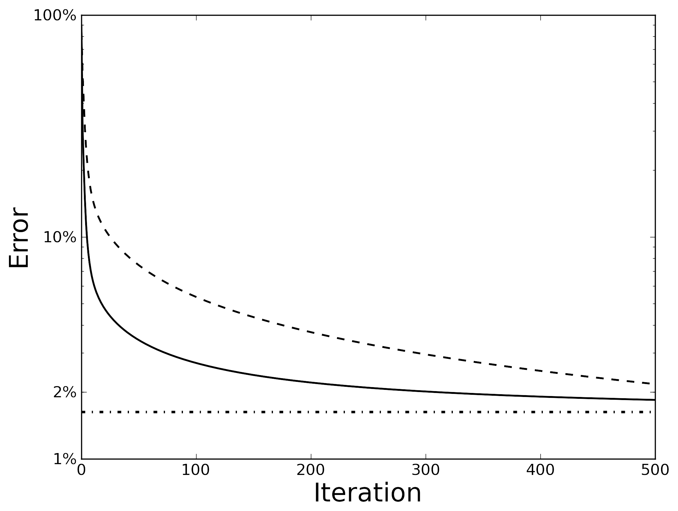
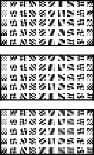
Figure 1: Results of the synthetic experiments. (left) Experiment for $K<d$ and $\tau=0$. The reconstruction error (solid line) converges to the optimal error (dash-dotted line) and the distance between $\boldsymbol{C}$ and $\boldsymbol{D}^{T}$ (dashed black) decades with it. (right) Synthetic experiments with a tight frame. From top to bottom, we show the original dictionary, the recovered dictionary $\boldsymbol{D}$ and recovered dual $\boldsymbol{C}^{T}$. The order in not necessarily the same as in the original, and some of the atoms could be inverted.

The first synthetic experiment has been performed with $K<d=25$ by generating $N=10^{4}$ training vectors as linear combinations of 15 random vectors. The data have been corrupted by additive Gaussian noise. We have run the algorithm with $K=15$, $\eta=1$ and a small $\ell_{2}$ regularization term on the coefficients $\boldsymbol{U}$, in order to ensure stability. In this setting we expected the algorithm to recover a dictionary close to the basis of the first 15 principal components, as well as converging to a dual $\boldsymbol{C}$ close to the transpose $\boldsymbol{D}^{T}$. In the experiments the distance between $\boldsymbol{D}$ and the PCA basis, assessed by the largest principal angle between the spanned subspaces, has decreased under $10^{-7}$ after very few iterations. In Figure 1, left image, we also show that the reconstruction error converges to the minimum achievable with the first $K$ principal components and that the dual $\boldsymbol{C}$ also converges to $\boldsymbol{D}^{T}$. The distance between $\boldsymbol{D}$ and its dual has been computed as the mean value of $1-|\boldsymbol{d}_{i}\cdot\boldsymbol{c}_{i}|/(\|\boldsymbol{d}_{i}\|\|\boldsymbol{c}_{i}\|)$ (where the $\boldsymbol{c}_{i}$ are the rows of $\boldsymbol{C}$).

In the second experiment we have constructed a tight frame, shown in Figure 1 (top, right), and generated $N=10^{4}$ training vectors as random superposition of 3 frame elements. The data have been again corrupted with additive Gaussian noise, and the algorithm run with $K=50$ (the same number of frame elements), $\eta=1$ and $\tau=0.5$. The reconstruction error has reached immediately the minimum achievable with the true generating frame, and the distance between the $\boldsymbol{C}$ and $\boldsymbol{D}^{T}$, computed as in the previous experiment, has got smaller than $10^{-2}$. In Figure 1 (right) we show the generating frame and compare it with the recovered dictionary $\boldsymbol{D}$ and dual $\boldsymbol{C}^{T}$. As apparent, most elements are present in both dictionaries (possibly inverted).

4.2 Benchmark datasets: digits and natural images

In the next experiments we have applied PADDLE to two sets of images widely used as benchmarks in computer vision: the Berkeley segmentation dataset [20] and the MNIST dataset [21]. The aim of this section is to offer a qualitative and quantitative assessment of the dictionaries recovered from these two classes of images, with realistic sizes of the training set.

Berkeley segmentation dataset

Following the experiment in [6, Sec. 4], we have extracted a random sample of $10^{5}$ patches of size 12x12 from the Berkeley segmentation data set [20]. The images intensities have been centered by their mean and normalized dividing by half the range (125). The patches have been separately recentered too.

We have run PADDLE over a range of values for $\tau$, and both with coding error ($\eta=1$) and without ($\eta=0$). The relative tolerance for stopping has been set to $10^{-4}$. The reconstruction error achieved at the various level of sparsity ($\tau$), both with and without the coding error, have been constantly lower than the reconstruction error achievable with a comparable number of principal components.
In Figure 2 we show images of the recovered dictionary, together with their duals. An interesting effect we report here is that different levels of sparsity in the coding coefficients also affects the visual patterns of the dictionary atoms. The more sparse is the representation the more the (very few) atoms tends to look like simple partial derivatives of a $2D$ Gaussian kernel, i.e. the dictionary tends to adapt poorly to the specific set of data. On the contrary, with a less sparse representation, a larger number of the atoms seem to encode for more structured local patterns or specific textures present in the dataset.

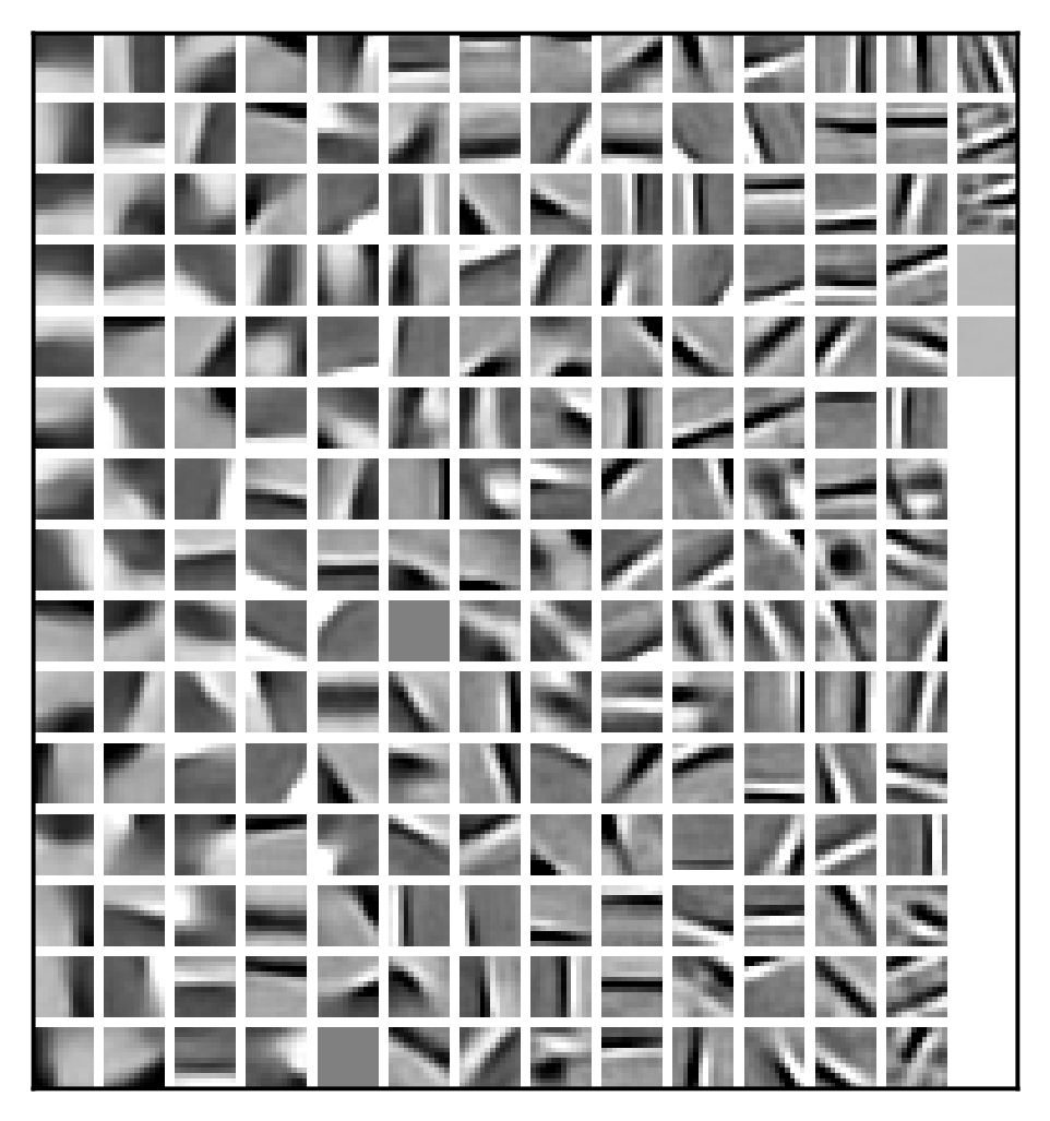
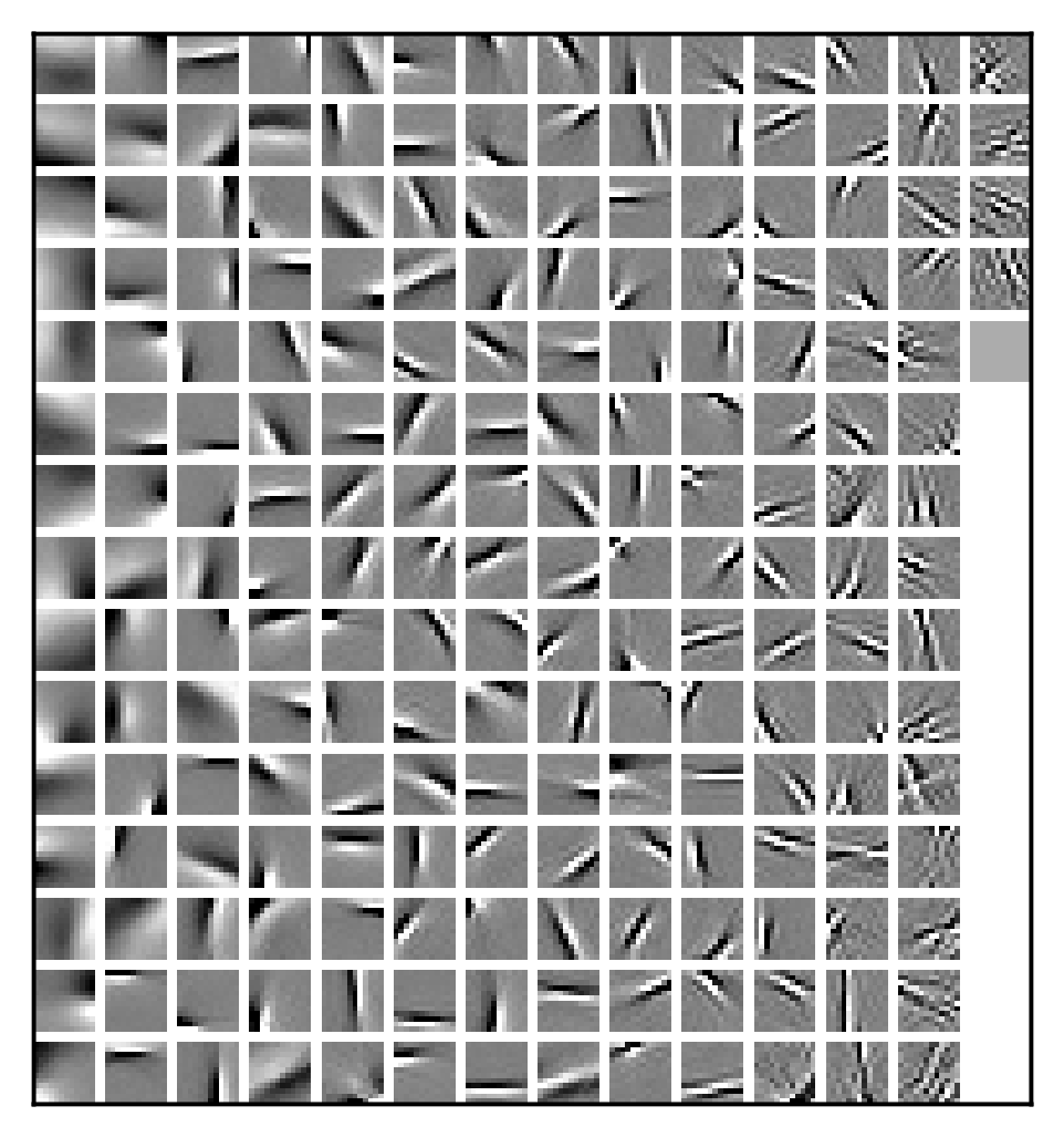
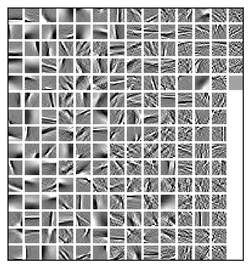
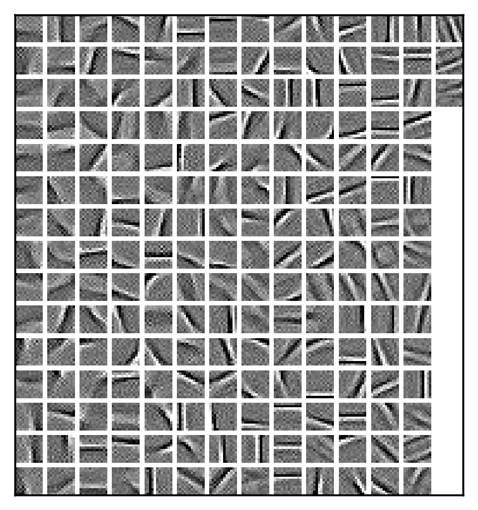
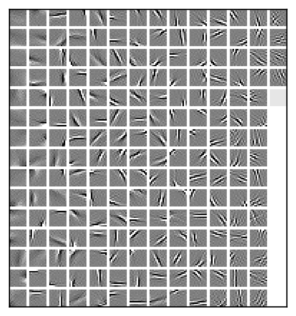
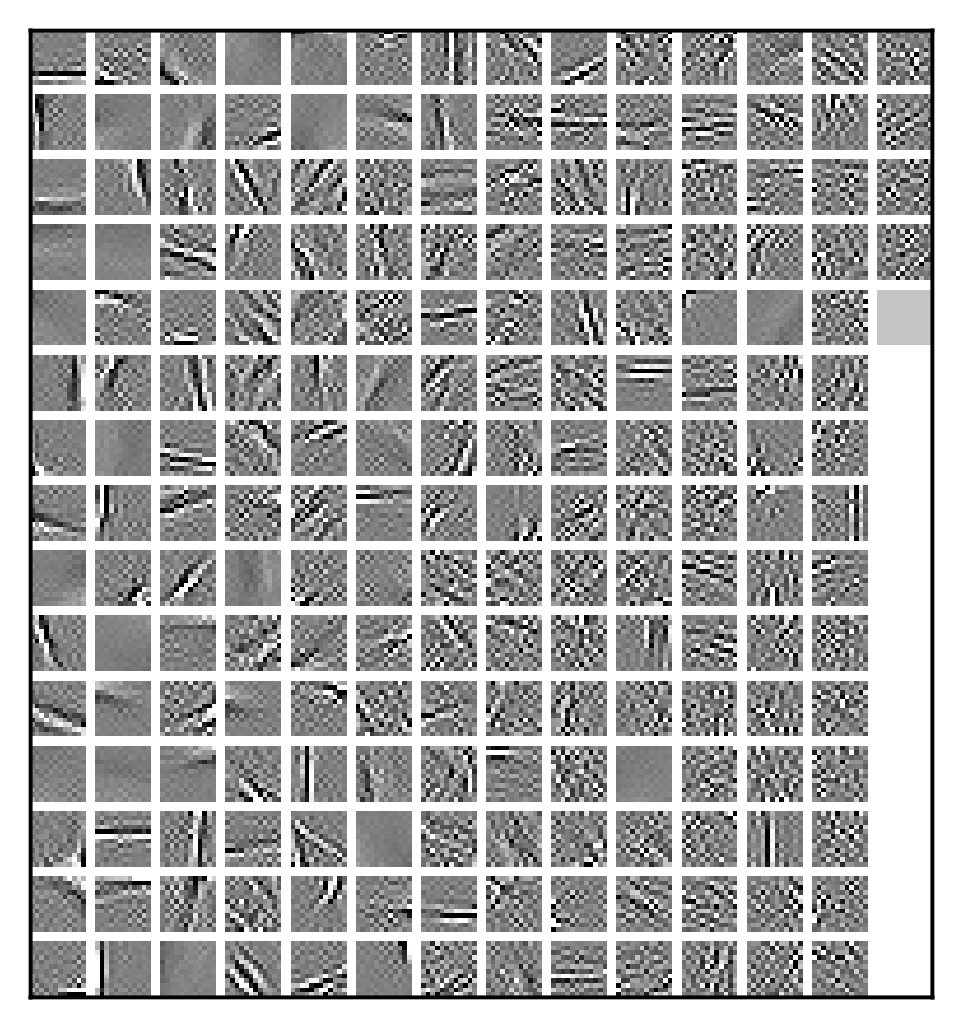
Figure 2: Decoding (top) and coding (bottom) matrices $\boldsymbol{D}$ and $\boldsymbol{C}$ learned from $100,000$ patches of size $12\times 12$ randomly sampled from the Berkley segmentation dataset. The dictionaries have been learned with different values of $\tau$: from left to right, $1$, $0.1$ and $0.02$. The atoms are in column-major order from the most used to the least one. The codes corresponding to the three dictionaries pairs uses on average 6.6, 65.9 and 139.8 atoms, respectively.

MNIST dataset

Next we have tested the algorithm on the $50,000$ training images of the popular MNIST data set [21], which is a collection of $28\times 28$ quasi binary images of handwritten digits. According to the experiments described in [6], we have trained the dictionary with $200$ atoms which is very likely to represent an overcomplete setting because the true dimensionality of the images is definitely less than $784$. All the images have been pre-processed by mapping their range into the interval $[0,1]$. The results obtained are consistent with those already reported in the literature. In particular, the learned dictionary $\boldsymbol{D}$ comprises the most representative digits from which it is possible to reconstruct all the others with a low approximation error. In Figure 3 (bottom) we show how the exemplar digit on the left can be expressed in terms of the small subset of the atoms in the middle, obtaining the approximate image on the right. As expected, the actual number of non-zero coefficients is extremely low if compared with the size of the dictionary. In the two rows in the middle, we first report all the dictionary atoms with non-zero coefficients and then we weight them with respect to their relevance in the reconstruction.
A second, more interesting aspect is the fast empirical convergence of the algorithm with such a well-structured dataset, as shown in Figure 3 (on the top). The initial dictionary has been built with random patches. After the first iteration it was already possible to inspect some digits, and the amount of change decreased rapidly reaching a substantial convergence after only a few iterations. The dictionary after $20$ iterations (corresponding to the full convergence) was almost identical to the one after $4$ iterations only.

Initialization	After $1$ iteration	After $4$ iterations	At convergence

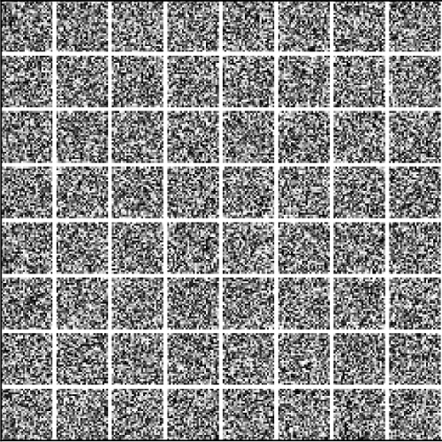
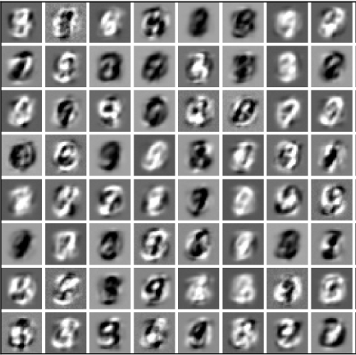
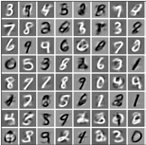
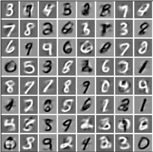
Figure 3: Experiments on MNIST dataset. See section 4.2 for details.

4.3 Classification

In this last group of experiments we have focused on the impact of using the dictionaries learned with the PADDLE algorithm in a classification context. More specifically, we have investigated the discriminative power of the sparse coding associated to the dictionary $\boldsymbol{D}$ and its dual $\boldsymbol{C}$ when used to represent the visual content of an image. The goal of the experiments has been to build a classifier to assign each image to a specific semantic class. In practice, we replicated the experimental setting of [22]. The classification results, reported in Table 1, show that the performance we have obtained using a representation computed with PADDLE is essentially the same – i.e. the results are not distinguishable within one standard deviation – as the one obtained with learned dictionary used by the authors in the original paper.

Encodings	$\boldsymbol{D}$	$\boldsymbol{C}$	[22]
Mean accuracy	0.987	0.984	0.985
Standard deviation	0.008	0.008	0.008

Table 1: Classification performances obtained on a subset of the popular Caltech101 dataset comprising two classes.

The results obtained with the dictionary $\boldsymbol{C}$ are especially encouraging if one consider the substantial gain in the computational time required to compute the sparse codes, with a fixed dictionary, for each new input image. In our experiments we have been able to process each image in less than $0.21$ seconds, while it took $2.3$ seconds per image, on the same machine, to use the implementation of the feature-sign search algorithm [4] provided with the software package ScSPM (available at http://www.ifp.illinois.edu/ jyang29/ScSPM.htm). Indeed, regardless the specific implementation of the sparse optimization method, it is easy to see that using $\boldsymbol{C}$ is always the best choice since it requires just one matrix-vector multiplication.

5 Conclusion

We have proposed a novel algorithm based on proximal methods to learn a dictionary and its dual, that can be used to compute sparse overcomplete representations of data. The experiments have shown that for image data the algorithm yields representations with good discriminative power. In particular, the dual dictionary can be used to efficiently compute the representations by means of a simple matrix-vector multiplication, without any loss of classification accuracy. We believe that our method is a valid contribution towards building robust and expressive dictionaries of visual features.

References

- [1] S. Mallat. A Wavelet Tour of Signal Processing. Academic Press, New York, 3rd edition, 2009.
- [2] B.A. Olshausen and D.J. Field. Sparse coding with an overcomplete basis set: A strategy employed by V1? Vision Research, 37(23):3311–3325, 1997.
- [3] M. Aharon, M. Elad, and A. Bruckstein. K-SVD: An algorithm for designing overcomplete dictionaries for sparse representation. Signal Processing, IEEE Transactions on [see also Acoustics, Speech, and Signal Processing, IEEE Transactions on], 54(11):4311–4322, 2006.
- [4] H. Lee, A. Battle, R. Raina, and A.Y. Ng. Efficient sparse coding algorithms. In Advances in Neural Information Processing Systems 19 (NIPS 2006), pages 801–808, 2006.
- [5] J. Mairal, F. Bach, J. Ponce, and G. Sapiro. Online learning for matrix factorization and sparse coding. Journal of Machine Learning Research, 11:19–60, Jan 2010.
- [6] M. Ranzato, C.S. Poultney, S. Chopra, and Y. LeCun. Efficient learning of sparse overcomplete representations with an energy-based model. In Advances in Neural Information Processing Systems 19 (NIPS 2006), 2006.
- [7] M. Ranzato, Y. Boureau, S. Chopra, and Y. LeCun. A unified energy-based framework for unsupervised learning. In Proc. of the 11-th International Workshop on Artificial Intelligence and Statistics (AISTATS 2007), Puerto Rico, 2007.
- [8] M. Ranzato, F.J. Huang, Y. Boureau, and Y. LeCun. Unsupervised learning of invariant feature hierarchies with applications to object recognition. In Proc. of Computer Vision and Pattern Recognition Conference (CVPR 2007), Minneapolis, 2007.
- [9] A. Beck and Teboulle. M. Fast gradient-based algorithms for constrained total variation image denoising and deblurring problems. IEEE Transactions on Image Processing, 18(11):2419–2434, 2009.
- [10] S. Becker, J. Bobin, and E. Candès. Nesta: A fast and accurate first-order method for sparse recovery, 2009.
- [11] P. L. Combettes and V. R. Wajs. Signal recovery by proximal forward-backward splitting. Multiscale Model. Simul., 4(4):1168–1200 (electronic), 2005.
- [12] I. Daubechies, M. Defrise, and C. De Mol. An iterative thresholding algorithm for linear inverse problems with a sparsity constraint. Communications on Pure and Applied Mathematics, 57:1413–1457, 2004.
- [13] Y. Nesterov. Smooth minimization of non-smooth functions. Math. Program., 103(1):127–152, 2005.
- [14] J. Duchi and Y. Singer. Efficient online and batch learning using forward backward splitting. Journal of Machine Learning Research, 10:2899–−2934, December 2009.
- [15] R. Jenatton, J. Mairal, G. Obozinski, and F. Bach. Proximal methods for sparse hierarchical dictionary learning. In Proc. of the 27th International Conference on Machine Learning, Haifa, Israel, 2010.
- [16] D. G. Luenberger. Linear and nonlinear programming. Kluwer Academic Publishers, Boston, MA, second edition, 2003.
- [17] L. Grippo and M. Sciandrone. On the convergence of the block nonlinear Gauss-Seidel method under convex constraints. Oper. Res. Lett., 26(3):127–136, 2000.
- [18] L. Rosasco, A. Verri, M. Santoro, S. Mosci, and S. Villa. Iterative projection methods for structured sparsity regularization. Technical Report MIT-CSAIL-TR-2009-050, CBCL-282, Center for Biological and Computational Learning (CBCL), MIT, Boston, MA, USA, 2009.
- [19] A. S. Nemirovsky and D. B. Yudin. Problem complexity and method efficiency in optimization. A Wiley-Interscience Publication. John Wiley & Sons Inc., New York, 1983. Translated from the Russian and with a preface by E. R. Dawson, Wiley-Interscience Series in Discrete Mathematics.
- [20] D. Martin, C. Fowlkes, D. Tal, and J. Malik. A database of human segmented natural images and its application to evaluating segmentation algorithms and measuring ecological statistics. In Proc. 8th Int’l Conf. Computer Vision, volume 2, pages 416–423, July 2001.
- [21] The MNIST database of handwritten digits. Http://yann.lecun.com/exdb/mnist/, 1998.
- [22] J. Yang, K. Yu, Y. Gong, and T. Huang. Linear spatial pyramids matching using sparse coding for image classification. In Proc. of Computer Vision and Pattern Recognition Conference (CVPR 2009), 2009.