Statistics of polymer extensions in turbulent channel flow

Abstract

We present direct numerical simulations of turbulent channel flow with passive Lagrangian polymers. To understand the polymer behavior we investigate the behavior of infinitesimal line elements and calculate the probability distribution function (PDF) of finite-time Lyapunov exponents and from them the corresponding Cramer’s function for the channel flow. We study the statistics of polymer elongation for both the Oldroyd-B model (for Weissenberg number $\mbox{Wi}<1$ ) and the FENE model. We use the location of the minima of the Cramer’s function to define the Weissenberg number precisely such that we observe coil-stretch transition at $\mbox{Wi}\approx 1$. We find agreement with earlier analytical predictions for PDF of polymer extensions made by Balkovsky, Fouxon and Lebedev [Phys. Rev. Lett. 84, 4765 (2000).] for linear polymers (Oldroyd-B model) with $\mbox{Wi}<1$ and by Chertkov [Phys. Rev. Lett. 84, 4761 (2000).] for nonlinear FENE-P model of polymers. For $\mbox{Wi}>1$ (FENE model) the polymer are significantly more stretched near the wall than at the center of the channel where the flow is closer to homogenous isotropic turbulence. Furthermore near the wall the polymers show a strong tendency to orient along the stream-wise direction of the flow but near the centerline the statistics of orientation of the polymers is consistent with analogous results obtained recently in homogeneous and isotropic flows.

I Introduction

Turbulent flows with polymer additives have been an active field of interest since the discovery toms49 of the phenomenon of drag reduction on the addition of small amounts (few parts per million) of long-chained polymers to turbulent wall-bounded flows. Polymers are long-chained complex molecules which have roughly spherical equilibrium configurations, known as the “coiled” state. In the simplest models of polymers, the relaxation of the polymers to the coiled state can be described by a single time scale $\tau_{\rm poly}$. If such a polymer is then placed in a straining flow, where the strain can be characterised by inverse of a time scale $\tau_{\rm fluid}$, the polymer can go from its coiled state to a stretched state if the ratio of the two time scales, the Weissenberg number $\mbox{Wi}>1$ squ05 . Thus in turbulent flows with strong strain the polymers can go through coil-stretch transition; the stretched polymers can then make significant contribution to the Reynolds stresses and this can result in drag-reduction lum73 ; hin77 . Hence to understand drag-reduction we must first understand the mechanism of coil-stretch transition. Also note that the back-reaction of the polymers to the flow becomes significant only when the polymers have undergone coil-stretch transition, thus to study coil-stretch transition itself, it may be safe to consider passive polymers.

There has been a large volume of work on coil-stretch transition of polymers in various kinds of flows. These works can be divided in four classes depending on the properties of the flow: (A) Individual polymer molecules advected by synthetic flows. In this class we first mention analytical works where the flows are either assumed to be random, smooth and white-in-time, Batchelor-Kraichnan flows (see e.g., deu92, ; bal+fux+leb00, ; che00, ; thi03, ; afo+vin05, ; tur07, ), or to have simple prescribed time dependence (e.g., Refs. lum73, ; mas+kon+sch+han93, ; mus+vin11, ). For $\mbox{Wi}<1$ the analytical works in Batchelor–Kraichnan flows have predicted that the probability distribution function (PDF) of polymer extension exhibits a power-law tail. Next are numerical works where the PDF of polymer extension and polymer tumbling times are calculated for polymers in various synthetic flows, including Batchelor-Kraichnan flows superimposed on uniform shearing background cel+pul+tur05 ; che+kol+leb+tur05 and models of a turbulent buffer layer  (e.g., sto+gra03, ). (B) Lagrangian polymers advected by solutions of the Navier–Stokes equation(see e.g., mas+kon+sch+han93, ; eck+kro+sch02, ; gup+sur+kho04, ; wat+got10, ). (C) Numerical simulations where the equations of polymers and fluids are solved simultaniously in two bof+cel+mus03 ; gup+per+pan12 and three (see e.g., per+mit+pan06, ; per+mit+pan10, ; dal+vas+hew10, ) spatial dimensions. (D) And finally numerical simulations of Lagrangian polymers in solutions of Navier–Stokes equations, in which the back-reaction from the polymers to the fluid is attempted to be incorporated dub04 ; Ter05 ; pet07 .

The simplest analytically tractable model is that of class (A) above. In this model the polymer is described by a simple bead-spring model,

$$\partial_{t}R_{\alpha}(t)=\sigma_{\alpha\beta}R_{\beta}+f(R)$$ (1)

where ${\bm{R}}$ is the end-to-end vector of a polymer (macro)molecule, $\sigma_{\alpha\beta}$ is a model for the velocity gradient matrix of the flow, $f(R)$ is the restoring force of the (entropic) spring in the bead-spring model, e.g.,$f(R)=-R/\tau_{\rm poly}$ for a harmonic overdamped spring (Oldroyd-B model), and $\tau_{\rm poly}$ the characteristic relaxation time of the polymer. The phenomenon of polymer stretching in flows is best understood by, for a moment, ignoring the restoring force in (1). The resulting equation is then the same equation as the one that describes the evolution of the infinitismal separation ($\delta{\bm{x}}$) between two fluid particles, i.e.,

$$\partial_{t}\delta x_{\alpha}=\sigma_{\alpha\beta}\delta x_{\beta}.$$ (2)

How two infinitesimally separated Lagrangian particles diverge in a turbulent flow has been a central topic in turbulence research for a long time. See, e.g., Ref fal+gaw+var01 for a recent review. Below we reproduce the essential points needed to apply such ideas to stretching of polymers in turbulence.

The growth (or decay) of the distance between two Lagrangian particles up to a time $T$ is described by the finite-time-Lyapunov-exponents(FTLEs) defined by

$$\mu_{\rm T}=\frac{1}{T}\ln\left[\frac{|\delta{\bm{x}}(t)|}{|\delta{\bm{x}}(t-T)|}\right].$$ (3)

For large $T$, $T\to\infty$ the PDF of FTLEs is conjectured to have a large deviation form bal+fux+leb00 ; eck+has+bra03 ; gaw08

$$P(\mu_{T})\sim\exp[-TS(\mu_{T})]$$ (4)

where $S(\mu_{T})$ is called the Cramer’s function or the entropy function. The simplest form of the entropy function is a parabola, of the form $S(\mu)=(\mu-\bar{\mu})^{2}/\Delta$, in which case (for each time $T$) the PDF of the FTLEs is a Gaussian distribution. The mean value of this Gaussian ($\bar{\mu}$) is an inverse time scale, $\bar{\mu}=1/\tau_{\rm fluid}$. For a turbulent (or random) flow the Weissenberg number is best defined by the ratio of $\tau_{\rm poly}/\tau_{\rm fluid}$. The analytical work of Ref. bal+fux+leb00 calculated the the PDF of polymer extensions in a random homogeneous flows with short correlation time. They found that for $\mbox{Wi}<1$ the PDF has power-law tail with an exponent $\alpha$. This exponent $\alpha$ can be obtained from the Cramer’s function $S(\mu)$ by solving the following set of coupled equations Eq. (5) and (6) given below,

$$\alpha = S^{\prime}(\beta+\frac{1}{\tau_{\rm poly}}-\bar{\mu})$$ (5)

$$S(\beta+\frac{1}{\tau_{\rm poly}}-\bar{\mu}) - \beta S^{\prime}(\beta+\frac{1}{\tau_{\rm poly}}-\bar{\mu})=0$$ (6)

Had the Cramer’s function been well approximated by a parabola of the form $S(\mu)=(\mu-\bar{\mu})^{2}/\Delta$, Eq. (5) would simplify to $\alpha=(2/\Delta)(1/\tau_{\rm poly}-\bar{\mu})$. Let us state here explicitly the assumptions that goes behind the derivation of Equations (5) and (6). The velocity gradient matrix is assumed to be short correlated in time, smooth in space and invariant under three dimensional rotation. In addition it is assumed that the PDF of FTLEs having a large deviation form holds true. Our numerical work, presented below, shows that both of these assumptions can be made for a three dimensional channel flow.

In this paper we calculate, the PDF of finite-time-Lyapunov exponents, for both short and large times, in turbulent channel flow by direct numerical simulation (DNS). We then show that at large time the PDF of FTLEs does satisfy a large deviation form with a Cramer’s function that can be approximated by a fourth–order polynomial. We further solve for the Oldroyd-B model of Lagrangian polymers in this flow. We use the location of the minima of the Cramer’s function, $\bar{\mu}$, as the inverse characteristic time scale of the fluid to define our Weissenberg number as

$$\mbox{Wi}\equiv\bar{\mu}\tau_{\rm poly}$$ (7)

Our simulations show a coil-stretch transition for $\mbox{Wi}\simeq 1$. For $\mbox{Wi}<1$, the PDF of polymer extension shows a power-law tail with scaling exponent $\alpha$. We find that the range of scaling shown by the PDF of polymer extensions depends on the wall-normal coordinate but the scaling exponent $\alpha$ is independent of the wall-normal coordinate. We further show that the exponent $\alpha$ satisfies (5) and (6).

For $\mbox{Wi}>1$ it is not possible to obtain a stationary PDF for the Oldroyd-B model. In this regime we use the nonlinear FENE (Finitely Extendable Nonlinear Elastic) model. For this model analytical work che00 has found that

$$\left\langle\frac{R}{R_{\rm max}}\right\rangle=-\frac{1}{\bar{\mu}}f(\left\langle R\right\rangle).$$ (8)

Our numerical simulations confirm this result. In addition we also find that the PDF of polymer extensions depends on the wall-normal coordinate, v.i.z, the polymer are more stretched near the wall than at the center of the flow. We further study the orientation of the polymers with respect to the channel geometry and the local velocity gradient tensor. Our results show that the orientation of the polymers is predominantly determined by the inhomogeneity of the flow, i.e., by the wall-normal coordinate as opposed to the local strain tensor. However, for polymers near the center of the channel we find that the orientation is also influenced by the principal directions of the rate-of-strain tensor, as has been seen in DNS of polymers in homogeneous isotropic flows jin+col07 ; wat+got10 .

The rest of the paper is organised as follows. In Section II we describe the equations we solve and the details of the numerical algorithm we use. Our results follow in Section III which is divided into three parts. The PDF of the finite-time-Lyapunov-exponents (FTLEs) are reported in Section III.1. The results described in this section are therefore independent of the polymer equation. The statistics of polymer extensions for the two models considered are presented in Section III.2 and III.3. The polymer orientation is characterized by calculating the correlations between the polymer end-to-end vector and fluid vorticity and the rate of strain tensor (Section III.4). The main conclusions of the study are summarized in Section IV.

II Equations and Numerical Methods

The fluid is described by the Navier–Stokes equations,

$$\partial_{t}{\bm{u}}+{\bm{u}}\cdot{\bm{\nabla}}{\bm{u}}=\nu\nabla^{2}{\bm{u}}+{\bm{\nabla}}p$$ (9)

with the incompressibility constraint,

$${\bm{\nabla}}\cdot{\bm{u}}=0.$$ (10)

Here ${\bm{u}}$ is the fluid velocity, $\nu$ the kinematic viscosity, and $p$ the pressure. We use the no-slip boundary condition at the walls and periodic boundary condition at all other boundaries. We have chosen our units such that the constant density $\rho=1$. The $x$ axis of our coordinate system is taken along the stream-wise direction, the $y$ axis along the wall-normal direction and $z$ axis along the span-wise direction. For brevity, we shall often use the common notation, $U\equiv u_{x}$, $V\equiv u_{y}$ and $W\equiv u_{z}$. The $x$, $y$ and $z$ dimensions of our channel are $L_{x}\times L_{y}\times L_{z}=4\pi\times 2\pi\times 2\pi$, with resolution ${\tt Nx}\times{\tt Ny}\times{\tt Nz}=128\times 129\times 128$.

The turbulent Reynolds number $Re_{\tau}={U_{\ast}}L/\nu=180$ is defined by the friction velocity ${U_{\ast}}=\sqrt{\sigma_{\rm w}}$ and $L\equiv L_{y}/2$, the half-channel width, where

$$\sigma_{\rm w}\equiv\nu\frac{\partial U}{\partial y}|_{\rm wall}$$ (11)

is the shear stress at the wall Mon+Yagv1 . In the following we non-dimensionalise velocity and distance by ${U^{+}}\equiv U/{U_{\ast}}$ and $y^{+}\equiv y/{y_{\ast}}$ respectively, using the friction length ${y_{\ast}}=\nu/{U_{\ast}}$. Time will also be measured in the unit of the large-eddy-turnover-time $\tau_{\rm L}\equiv(U^{\rm center}/L)^{-1}$, where $U^{\rm center}$ is average streamwise velocity at the center of the channel. The large-scale Reynolds number defined by $\mbox{Re}={U_{0}}L/\nu=4200$ where ${U_{0}}$ is the centreline streamwise velocity for the laminar flow of same mass flux.

We solve Eqs. (9) and (10) by using the SIMSON SIMSON code which uses a pseudo-spectral method in space (Chebychev-Fourier). For time integration a third-order Runge-Kutta method is used for the advection term and the uniform pressure gradient term. The viscous term is discretized using a Crank-Nicolson method mos+kim+man99 . In Fig. (1a) we show a visualization of the vortical structures from a typical snapshot of our simulation. In Fig. (1b) we plot $\left\langle{U^{+}}\right\rangle$ as a function of $y^{+}$ at the stationary state of our simulations, where $\left\langle\cdot\right\rangle$ denotes averaging over the coordinate directions $x$ and $z$ and over time. Further details about the code validation can be found in Ref. Far10 ; sar+sch+bra+pic+cas12 .

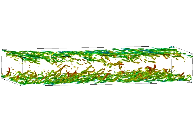
Figure 1: (Colour online) (a) Visualization of vortical structures in our simulation. The structures are identified by negative values of the second largest eigenvalue of the matrix $S_{ik}S_{kj}+\Omega_{ik}\Omega_{kj}$ where $S_{ij}$ and $\Omega_{ij}$ and the symmetric an anti-symmetric part of the velocity gradient matrix jeo+hus+sch+kim97 . The vortical structures are located close to the walls. (b) Normalised mean stream-wise velocity $\left\langle U^{+}\right\rangle$ versus the wall-normal coordinate $y^{+}$ plotted for one half of the channel.

We use a Lagrangian model for the polymers where we solve one stochastic differential equation (SDE) for each polymer molecule. This model uses several approximations which are as follows Bir87 ; Pha02 : (A) The centre-of-mass of a polymer molecule follows the path of a Lagrangian particle. (B) Even when fully stretched the polymer molecule is very small compared to the smallest scales of turbulence. This approximation is well justified hin77 . (C) A polymer molecule is modelled by two beads separated by a vector which represents the end-to-end distance of the polymer molecule. (D) The forces acting on the beads are stokes drag, restoring force of an overdamped spring with time scale $\tau_{\rm poly}$, and thermal noise. To be specific, we track $N_{\rm p}=2.16\times 10^{5}$ Lagrangian passive tracers in the flow by solving

$$\partial_{t}{\bm{r}}^{\rm j}(t|t_{0},{\bm{r}}^{j}_{0})={\bm{v}}^{\rm j}(t|t_{0},{\bm{r}}^{j}_{0})\/.$$ (12)

Where ${\bm{r}}^{\rm j}(t|t_{0},{\bm{r}}^{j}_{0})$ is the position of the $j$-th Lagrangian particle which was at position ${\bm{r}}^{\rm j}_{0}$ at time $t_{0}$ and ${\bm{v}}^{\rm j}(t|t_{0},{\bm{r}}^{j}_{0})$ is its velocity with $j=1,\ldots,N_{\rm p}$. The Lagrangian velocity of a particle, which is generally at an off-grid point, is obtained by tri-linear interpolation from Eulerian velocity at the neighboring grid points. Equation (12) is integrated by a third order Runge-Kutta scheme. Each of these Lagrangian particles represent a polymer molecule. For $j$-th Lagrangian particle the vector representing the end-to-end distance is denoted by $R^{\rm j}$ and obeys the following dynamical equation:

$$\partial_{t}R^{\rm j}_{\alpha}(t)=\sigma^{\rm j}_{\alpha\beta}R^{\rm j}_{\beta}+f(R^{\rm j})+\sqrt{\frac{2R^{2}_{0}}{3\tau_{\rm poly}}}B^{\rm j}_{\alpha}\/.$$ (13)

Here $\sigma^{\rm j}_{\alpha\beta}=\partial_{\beta}{\bm{v}}^{\rm j}(t|t_{0},{\bm{r}}^{j}_{0})_{\alpha}$, $f(R^{\rm j})$ is the restoring force of the polymer, $\tau_{\rm poly}$ is the characteristic decay time of the polymer and ${\bm{B}}^{\rm j}$ is a Gaussian random noise with $\left\langle B_{\alpha}\right\rangle=0$ and $\left\langle B_{\alpha}(t)B_{\beta}(t^{\prime})\right\rangle=\delta_{\alpha\beta}\delta(t-t^{\prime})$. The prefactor of the random noise is chosen such that in the absence of external flow, i.e., $\sigma^{\rm j}_{\alpha\beta}=0$, the polymer attains thermal equilibrium, $\left\langle R^{\rm j}_{\alpha}R^{\rm j}_{\beta}\right\rangle=R^{2}_{0}\delta_{\alpha\beta}/3$. Here $\left\langle\cdot\right\rangle$ denotes averaging over the noise ${\bm{B}}$. For the linear Oldroyd-B model $f(R)=-R/\tau_{\rm poly}$. For the FENE model $f(R)=-R/\tau_{\rm poly}\{1-(R/R_{\rm max})^{2}\}$. Eq. (13) is also solved by a third order Runge-Kutta scheme except for the noise which is integrated by an Euler-Maruyama method hig01 .

To compare with the analytical theory of Ref. bal+fux+leb00 we also need to calculate the PDF of finite-time Lyapunov exponents of Lagrangian particles in this flow. For this we need to calculate the rate at which two infinitismally separated Lagrangian particles diverge as time progresses. For this purpose we also calculate the evolution of an infinitesimal vector in our turbulent flow, given by the equations,

$$\partial_{t}\delta x^{\rm j}_{\alpha}=\sigma^{\rm j}_{\alpha,\beta}\delta x^{\rm j}_{\beta}.$$ (14)

Where $\delta{\bm{x}}^{\rm j}$ is a vector carried by the $j$-th Lagrangian particle. This is of course the same equation obeyed by a Lagrangian polymer, [Eq. (13)], if the restoring force of the polymer and the Brownian noise are omitted.

The correspondence between our Lagrangian description and the Eulerian description of polymeric fluids is that in the latter the dynamical variable for the polymers is the symmetric positive definite (SPD) tensor $C_{\alpha\beta}\equiv\left\langle R_{\alpha}R_{\beta}\right\rangle$. A DNS of the Eulerian description has certain difficulties vai03 ; vai06 ; per+mit+pan06 ; per+mit+pan10 . Firstly the numerical schemes used must preserve the symmetric and positive-definite (SPD) nature of $C_{\alpha\beta}$. Secondly for high Weissenberg numbers large gradients of $C_{\alpha\beta}$ can develop which can lead to numerical instabilities. Stability can generally be restored by employing either shock-capturing schemes vai06 ; Per09 ; per+mit+pan10 ; dal+vas+hew10 or by introducing dissipation in the Eulerian description of the polymer ben03 ; ang05 . Lagrangian methods dub04 ; Ter05 are generally able to avoid such numerical pitfalls and can attain a higher Weissenberg number. On the other hand it is quite straightforward to incorporate the back-reaction of the polymer into the flow in the Eulerian model but is tricky in the Lagrangian model Ter05 ; pet07 . Note finally that more complicated Lagrangian models have also been employed where a single polymer is represented by a chain of beads connected by springs jin+col07 ; wat+got10 .

III Results

III.1 Finite-time Lyapunov Exponents

To calculate the PDF of FTLEs we integrate Eq. (14) for each Lagrangian particle over a finite time interval $T$ and compute the the finite-time Lyapunov exponent (FTLE) as

$$\mu_{\rm T}^{\rm j}=\frac{1}{T}\ln\left[\frac{|\delta{\bm{x}}^{\rm j}(t)|}{|\delta{\bm{x}}^{\rm j}(t-T)|}\right].$$ (15)

Below we present the analysis of the PDF of FTLEs for channel flows.

Since the channel flow is not homogeneous in the wall-normal direction the statistics can, in principle, depend on $y^{+}$. Hence we label our particles by their wall-normal coordinate ($y^{+}$) at the final position, i.e., at time $T$. While integrating the equations for $\delta{\bm{x}}^{\rm j}$, Eq. (14), we store the evolution of $\delta{\bm{x}}^{\rm j}$ and use this to calculate $\mu_{\rm T}^{\rm j}$ for each of $\delta{\bm{x}}^{\rm j}$. To calculate the PDF of $\mu_{\rm T}$ we gather statistics in two different ways. First we calculate the PDF of $\mu_{\rm T}$ for all particles at a fixed $y^{+}$. Furthermore we run our simulations over several $T$ and after each time interval $T$ the particles are redistributed uniformly across the channel and their initial separation vector $\delta{\bm{x}}^{\rm j}(t=0)$ oriented randomly. By definition then we generate a $P(\mu_{\rm T},y^{+})$ which depends on $y^{+}$. The PDFs for two different values of $y^{+}$, one close to the wall, and one near the centerline, are respectively plotted in Figs. (2a) and (2b) for several time intervals $T$. The peak and mean of the PDFs are always positive showing that it is more probable for $|\delta{\bm{x}}^{\rm j}|$ to increase exponentially as a function of time. For small $T$ the PDFs near the center and the PDF near the wall are very different from each other. Significantly larger elongation is found for those elements that are located closer to the wall. However, the two PDFs approach each other for large $T$. This can also be seen by plotting the mean value of the PDFs for three different $y^{+}$s as a function of time, Fig. (3). The peak value also shows a similar trend, see the inset in Fig. (3). Hence an unique Cramer’s function independent of $y^{+}$ can be defined for the channel flow for only very large time when the PDFs for different $y^{+}$ merge with one another. In a channel flow the stress tensor $\sigma_{\alpha\beta}$ depends strongly on the wall-normal coordinate. Thus for short $T$ we can expect that the PDF of $\mu_{\rm T}$ depend of $y^{+}$. Conversely, when $T$ becomes much larger than the typical time it takes for a particle to travel from a position near the wall to a position near the center line, we expect $\mu_{\rm T}$ to be independent of $y^{+}$. Let us call this typical time the exit time $T_{\rm exit}$. Surprisingly, we observe from our data that we need to have $T_{\rm exit}\gtrsim 80\tau_{\rm L}$ for $\mu_{\rm T}$ to be independent of $T$. An estimate of the time it takes for a particle to travel from the wall to the center of the channel can be given by the ratio of the half-width of the channel to the friction velocity, $T_{\rm friction}\equiv(L_{y}/2)/{U_{\ast}}\approx 15$ in our simulations. In units of this time $T_{\rm exit}\gtrsim 5T_{\rm friction}$ which provides a better estimate than $\tau_{\rm L}$.

From the PDF of $\mu_{\rm T}$ for large $T$ we calculate the Cramer’s function using Eq. 4. We normalise $P(\mu_{\rm T})$ such that its integral over the range of $\mu_{\rm T}$ is unity. For $T>T_{\rm exit}$ the Cramer’s functions $S(\mu)$ calculated at different times $T$ are found to be independent of $T$ as it should be. This is shown by the collapse of the Cramer’s function calculated at different times for a fixed $y^{+}=62$ in Fig. (4). This proves that the conjecture in Equation (4) hold true. Furthermore, the Cramer’s function thus found is independent of $y^{+}$. The Cramer’s function has earlier been calculated from DNS of two bof+cel+mus03 - and three bec+bif+bof+cen+mus+tos06 dimensional homogenous isotropic turbulence, turbulence in the presence of homogeneous shear eck+kro+sch02 , and for hydromagnetic convection kur+bra91 . This is the first time is has been calculated for a channel flow.

The connection between the Cramer’s function and the PDF of end-to-end polymer distance was shown in Ref bal+fux+leb00 for linear polymers and in Ref che00 for nonlinear polymers. We discuss such relations in the next section where it will turn out to be useful to have an algebraic expression for the Cramer’s function. In the simplest case the Cramer’s function is a parabola which implies that the PDF of FTLEs is a Gaussian distribution. It is clear from Fig. (4) that in our case $S(\mu)$ is not well approximated by a parabola except for $\mu\approx\bar{\mu}$. The departure from Gaussianity is characterized by higher (than second) power of $\mu$ in a polynomial expansion of $S(\mu)$. The next level of approximation would be to use a fourth–order polynomial for the following two reasons: (a) The function $S(\mu)$ in Fig. (4) is clearly not symmetric about its axis, hence we need an odd power of $\mu$ to approximate it. (b) The function $S(\mu)$ must be convex hence the highest power of $\mu$ appearing in $S(\mu)$ must be even. Hence we use fit the fourth-order polynomial,

$$S(\mu)=a_{2}(\mu-\bar{\mu})^{2}+a_{3}(\mu-\bar{\mu})^{3}+a_{4}(\mu-\bar{\mu})^{4},$$ (16)

to our numerical data for $S(\mu)$ averaged over all values of $y^{+}$ and extract the coefficients $a_{2},a_{3}$, and $a_{4}$ above. To estimate the errors in the coefficients $a_{k}$ we use the same fit to $S(\mu)$ obtained for individual $y^{+}$ and quote the range of $a_{k}$ obtained from such fits as the error in $a_{k}$. The best fit is also plotted in Fig. (4). The coefficients corresponding to the best fit and their errors are given in the caption of Fig. (4).

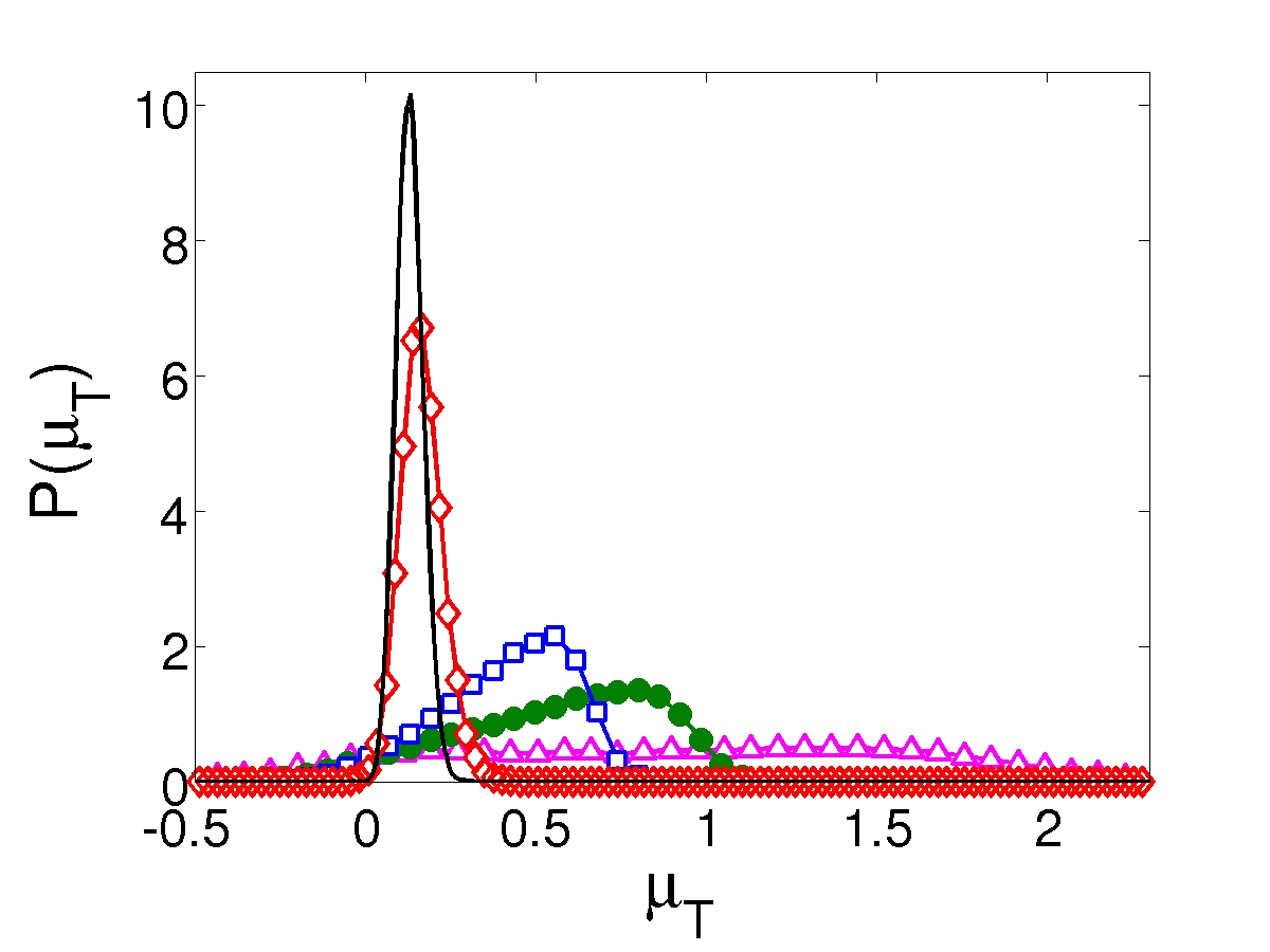
Figure 2: (Colour online) (a) PDF of $\mu_{\rm T}$ near the wall ($y^{+}\approx 6$) for several values of $T$, v.i.z, $T=1.(\vartriangle)$, $3.(\bullet)$, $5.(\square)$, $35.(\lozenge)$, and $100.(-)$. (b) PDF of $\mu_{\rm T}$ near the centerline ($y^{+}\approx 180$) for several values of $T$, v.i.z, $T=1.(\vartriangle)$, $3.(\bullet)$, $5.(\square)$, $35.(\lozenge)$, and $100.(-)$. Plots at other intermediate values of $T$ are consistent with this plot, but are not show here for clarity. All times are measured in the unit of $\tau_{\rm L}$.

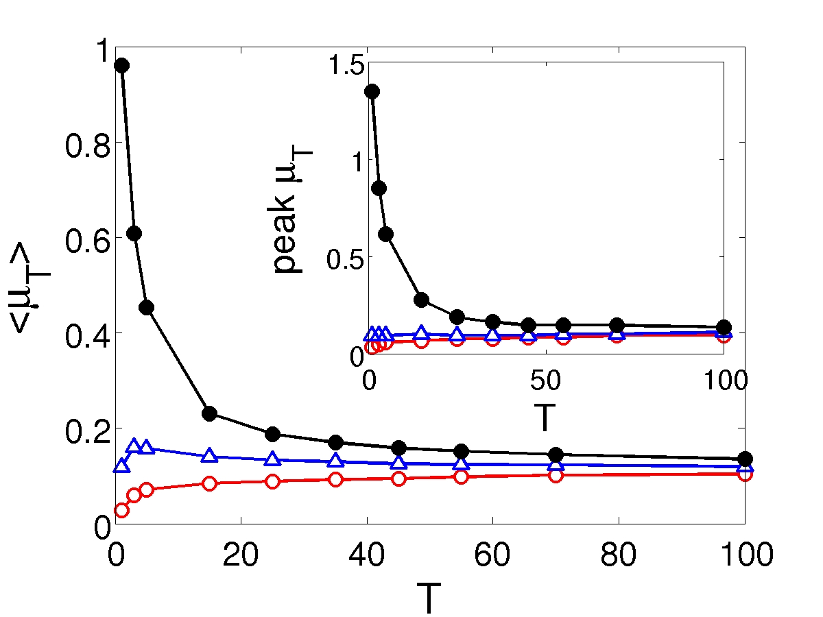
Figure 3: (Color online) Mean FTLE $\left\langle\mu_{\rm T}\right\rangle$ versus $T$ for three different positions, in the channel, near the wall(•), near centerline ($\circ$) and at $y^{+}=84$ ($\vartriangle$). All times are measured in the units of $\tau_{\rm L}$.

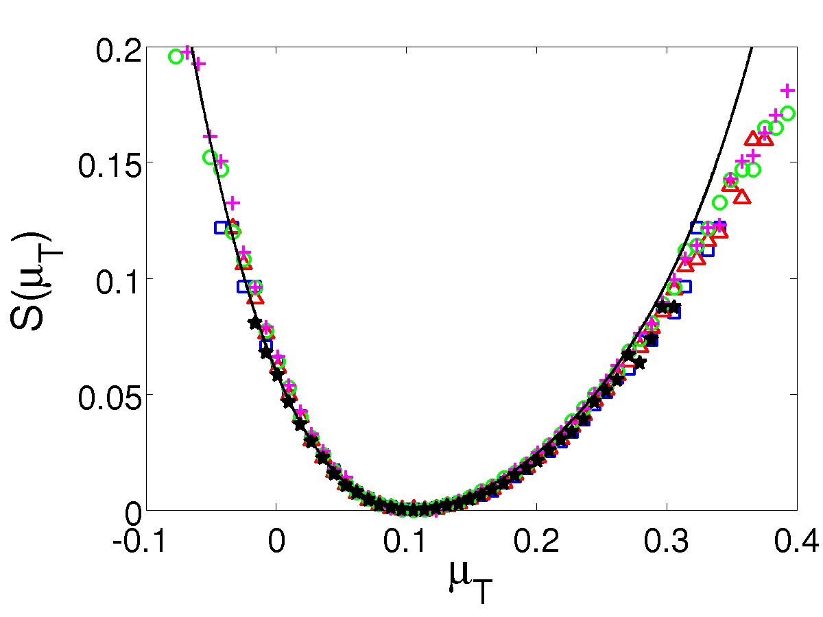
Figure 4: (Color online) The collapse of the Cramer’s functions $S(\mu)$ versus $\mu$ at $y^{+}=62$ for different times $T$, v.i.z, $T=35.(+),45.(\circ),55.(\vartriangle),70.(\square)$, and $100.(\star)$. All times are measured in the units of $\tau_{\rm L}$. The continuous line is the polynomial fit as given in Eq. 16 with $\bar{\mu}=0.105[0.088\ \ 0.13]$ and $a_{2}=3.55[3.09\ \ 4.35]$, $a_{3}=-12.60[-27.48\ \ -4.29]$ and $a_{4}=39.64[3.84\ \ 90.07]$. We have used the same polynomial form to fit $S(\mu)$ obtained for individual $y^{+}$. The maximum and minimum values of the fitting parameters are given inside square brackets.

III.2 Statistics of polymer extensions: Oldroyd-B model

Before we present detailed results on statistics of polymer extension let us precisely define the Weissenberg number, Wi. In simulations the Weissenberg number is defined as the ratio of the characteristic time-scale of the polymer, $\tau_{\rm poly}$ over a characteristic time scale of the fluid. Different definitions of the characteristic time scale for fluid has been used in literature to define the Weissenberg number. Refs. per+mit+pan06 ; jin+col07 ; wat+got10 use the Kolmogorov time scale $\tau_{\eta}$ to define the Weissenberg number. We denote this Weissenberg number by $\mbox{Wi}_{\eta}=\tau_{\rm poly}/\tau_{\eta}$ where $\tau_{\eta}$ is the Kolmogorov time scale. In this paper we principally use the following definition for Weissenberg number

$$\mbox{Wi}\equiv\bar{\mu}\tau_{\rm poly}$$ (17)

where $\bar{\mu}$ is the location of the minima of the Cramer’s function $S(\mu)$. Our choice has two principal advantages. Firstly in channel flows the Kolmogorov scale depends on the wall-normal coordinate and hence is not unique. Secondly and more importantly a proper choice of Weissenberg number gives the coil-stretch transition of the polymer at $\mbox{Wi}\approx 1$ which is exactly what we obtain. To compare with earlier simulations, which were all done in homogeneous flows, we also calculate $\mbox{Wi}^{\rm wall}_{\eta}$ and $\mbox{Wi}^{\rm center}_{\eta}$, where we use the Kolmogorov time scale at the wall and at the center of the flow respectively. We typically obtain, $\mbox{Wi}^{\rm wall}_{\eta}\approx 30\mbox{Wi}$ and $\mbox{Wi}^{\rm center}_{\eta}\approx 5\mbox{Wi}$. The different values of Wi that we use are given below, in parentheses we give the corresponding values of $\mbox{Wi}^{\rm center}_{\eta}$ for easy comparison with earlier simulations of homogeneous and isotropic turbulence. For the Oldroyd-B model, $\mbox{Wi}(\mbox{Wi}^{\rm center}_{\eta})=0.1(0.5)$, $0.2(1)$,$0.3(1.5)$, and $0.5(2.5)$ and $\mbox{Wi}(\mbox{Wi}^{\rm center}_{\eta})=0.1(0.5)$, $0.3(1.5)$,$0.5(2.5)$,$1.5(7.5)$, $2.5(12.5)$,$3.5(17.5)$,$4.5(22.5)$,$5.5(27.5)$,$7(35)$, and $10(50)$ for the FENE model. We use $R_{0}=10^{-7}$, $10^{-8}$, and $R_{\rm max}/R_{0}=100$ and $1000$ for the FENE model.

Let us first present the results for the Oldyroyd-B model. Here we expect to see a power-law behavior for the PDF of polymer extensions, $Q(R)\sim R^{-\alpha-1}$ bal+fux+leb00 for large $R$. In general, the calculation of PDFs from numerical data is plagued by errors originating from the binning of the data to make histograms. Thus it is often a difficult task to extract exponents such as $\alpha$ from such PDFs. A reliable estimate of such an exponent can be obtained by using the rank-order method mit05a to calculate the corresponding cumulative probability distribution function,

$$Q^{c}(R)\equiv\int_{0}^{R}Q(\xi)d\xi$$ (18)

If the PDF has a scaling range the cumulative PDF also shows scaling, i.e., $Q^{c}(R)\sim R^{-\alpha}$. These cumulative PDFs are plotted in Fig. (5) for different values of Wi at fixed wall distance $y^{+}=74$ The cleanest power-law is seen for $\mbox{Wi}=0.5$. So we choose this Weissenberg number for further detailed investigation. First we show that the exponent of the power-law ($\mbox{Wi}=0.5$) $\alpha=0.81\pm 0.02$ does not depend on the $y^{+}$ although the range over which scaling is obtained does, Fig. (6). The exponent $\alpha$ is obtained by fitting a power-law for five different values of $y^{+}$. The mean is reported as the exponent above and the standard deviation from the mean is reported as the error.

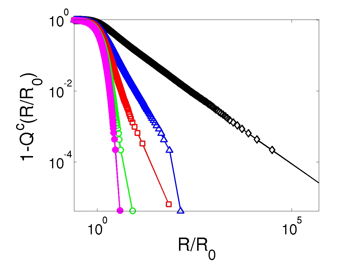
Figure 5: (Color online) Log-log plot of the cumuliative PDF $Q^{c}(R)$ of the polymer extensions $R$ as a function of $R$ for different values of Wi, v.i.z, $\mbox{Wi}=0.05($•$),0.1(\circ),0.2(\square),0.3(\vartriangle)$, and $0.5(\lozenge)$.

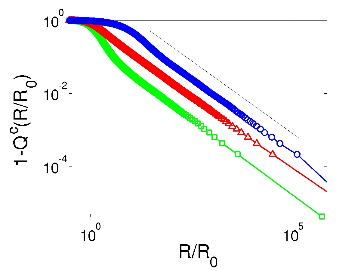
Figure 6: (Color online) Log-log plot of the cumuliative PDF $Q^{c}(R)$ of the polymer extensions $R$ as a function of $R$ for different $y^{+}$, v.i.z, $y^{+}=8(\circ),74(\vartriangle)$, and $180(\square)$. We fit a straight line to the data between the two dashed vertical lines to calculate $\alpha$. This fit is shown as the black line.

This exponent $\alpha$ can be obtained from the Cramer’s function $S(\mu)$ using the set of couple equations Eq. (5) and (6) bal+fux+leb00 which we rewrite below,

$$\alpha=S^{\prime}(\beta+\frac{1}{\tau_{\rm poly}}-\bar{\mu})$$ (19)

where $\beta$ must be obtained by solving the differential equation,

$$S(\beta+\frac{1}{\tau_{\rm poly}}-\bar{\mu})-\beta S^{\prime}(\beta+\frac{1}{\tau_{\rm poly}}-\bar{\mu})=0$$ (20)

Had the Cramer’s function been well approximate by a parabola of the form $S(\mu)=(\mu-\bar{\mu})^{2}/\Delta$, Eq. (5) would simplify to $\alpha=(2/\Delta)(1/\tau_{\rm poly}-\bar{\mu})$. We have checked that this quadratic approximation does not give accurate result for $\alpha$ in our case. Using the algebraic expression for $S$ given in Eq. 16, we numerically solve Eqs. (5) and (6). This give $\alpha=0.9\pm 0.29$ which agrees with the results obtained from the cumulative PDF of polymers within error bars. We note here that the $\alpha$ we calculate using the Cramer’s function has large margin of error because the $\alpha$ depends sensitively on the coefficients $a_{k}$ in Eq. 16. To find these coefficients accurately we need to know the Cramer’s function accurately for a large range of its argument not just the location of its minima. Numerically this is a difficult task and would require collecting data over very long times.

Finally let us comment on the possible experimental determination of the exponent $\alpha$. In practice no polymers are linear and in most cases the ratio of $R_{\rm max}$ (maximum possible extension of the polymer) to $R_{0}$ (the equilibrium length) ranges between $100$ and $1000$. To see the effect of a maximum extension, we first select one of the cumulative PDFs plotted in Fig. (6), say for $y^{+}=74$. From this cumulative PDF we remove all the polymers for which $R$ is so large that $R/R_{0}>R_{\rm cutoff}$ where we choose $R_{\rm cutoff}=100$ and $1000$. The resultant cumulative PDFs are plotted in Fig. (7) where the original cumulative PDF is also plotted for comparison. It can be seen that the scaling behavior, although present, is valid over a much smaller range. In the same figure we have also plotted the cumulative PDF for the FENE model with $R_{\rm max}/R_{0}=1000$. This also shows scaling with a reduced range. Thus we expect that in experiments similarities to this scaling law should be visible although it may be difficult to detect because of a reduced range of scaling.

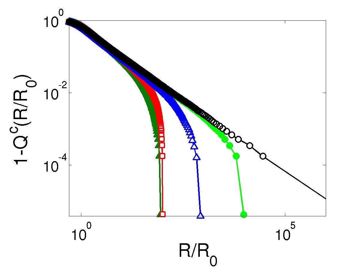
Figure 7: (Color online) The cumulative PDF $Q^{c}(R)$ of the polymer extensions $R$ as a function of $R$ for the Oldroyd-B model ($\circ$), Oldroyd-B model with all polymers with $R/R_{\rm max}>R_{\rm cutoff}$ removed with $R_{\rm cutoff}=10^{4}($•$)$ and $R_{\rm cutoff}=100(\square)$, FENE model with $R_{\rm max}/R_{0}=10^{3}(\vartriangle)$ and with $R_{\rm max}/R_{0}=10^{2}(\blacktriangle)$.

III.3 Statistics of polymer extensions: FENE model

So far we have described the polymer statistics for $\mbox{Wi}\leq 0.5$. As we increase the Wi and make it close to unity no stationary statistics of the polymers is obtained. We interpret this by noting that we are close to the coil-stretch transition. A stationary state can be obtained either by including the feedback from the polymers into the fluid or by using nonlinear polymers e.g., the FENE model. We choose the second option. In the FENE model we have used $R_{\rm max}/R_{0}=100$ and $1000$. Our results as reported below does not depend on this parameter.

Let us first consider the mean extensions of the polymers averaged over the whole channel as a function of the Weissenberg number. Using a saddle point approximation Chertkov che00 has shown that for $\mbox{Wi}>1$ the mean polymer extension obeys the implicit relation

$$\left\langle\frac{R}{R_{\rm max}}\right\rangle=-\frac{1}{\bar{\mu}}f(\left\langle R\right\rangle)$$ (21)

where $f$ is the FENE force. In Fig 8 we show that we obtain reasonable agreement between between this analytical prediction and our numerical results for different values of the Wisenberg number. The error-bars in this plot are the variance of the polymer extension calculated over the channnel.

Let us now consider the full PDF of the polymer extension. In Fig. (9) we plot the PDF for three different values of the Weissenburg number, $\mbox{Wi}=0.5$, $1.5$ and $10$. The coil-stretch transition is clearly demonstrated in this figure. For $\mbox{Wi}=0.5$ the PDF is peaked near zero which corresponds to the coiled state. For $\mbox{Wi}=1.5$ the peak of the PDF is still close to zero but the PDF is well spread over the whole range. At $\mbox{Wi}=10$ the PDF has a peak near $R_{\rm max}$; this is the stretched state of the polymer. In this Figure we have plotted the PDFs for $y^{+}=74$. The PDF at other wall-normal coordinates in the channel shows the same qualitative nature. Similar plots of the PDF of polymer extensions but for a simple model of polymers in uniform shear has been obtained in Ref. che+kol+leb+tur05 . A more careful scrutiny, however, reveals differences between our results and that of Ref. che+kol+leb+tur05 for $\mbox{Wi}=10$. In particular, we do not observe the plateau in the PDF seen in Fig 2 of Ref. che+kol+leb+tur05 . However, it is possible to observe a power-law behavior of the left-tail of the PDF as shown in Fig. 10. Plots of the PDF of polymer extensions have also been recently obtained in experiments liu+ste10 . For strong shear the experiments results have qualitative agreement with the results of Ref. che+kol+leb+tur05 including the presence of the plateau, although quantitative agreement is still lacking. The disagreements of our results with that of Ref. che+kol+leb+tur05 might be due to spatial inhomogeineity of channel flow compared to the case of uniform shear.

The effects of spatial inhomogeneity is also seen in Fig. (11), where we show how the mean polymer extension $\left\langle R\right\rangle_{xz}$, where the averaging is over the stream-wise and the span-wise direction, changes with Wi across the channel for $R_{\rm max}/R_{0}=100$. For a given Wi the average polymer extension is small near the wall, increases to a maximum around $y^{+}\approx 10$ (this corresponds to the region of maximum strain), and then decreases towards the center of the domain where the flow is close to homogeneous turbulence. A similar trend is also seen for $R_{\rm max}/R_{0}=1000$. This trend has been seen in earlier DNS of polymeric turbulence in channel flows (see e.g., whi+mun08, , and references therein). Note however that for larger values of Wi the average polymer extension becomes almost uniform across the channel (except very near the wall where it is always small). This is because the polymers that are stretched close to the wall on reaching the centerline are not able to relax fast enough because the polymer relaxation time scales are much larger than the fluid time scales. The maximum extension increases as a function of Weisenberg number for small Weisenberg numbers and saturates for higher values, see Fig. 12.

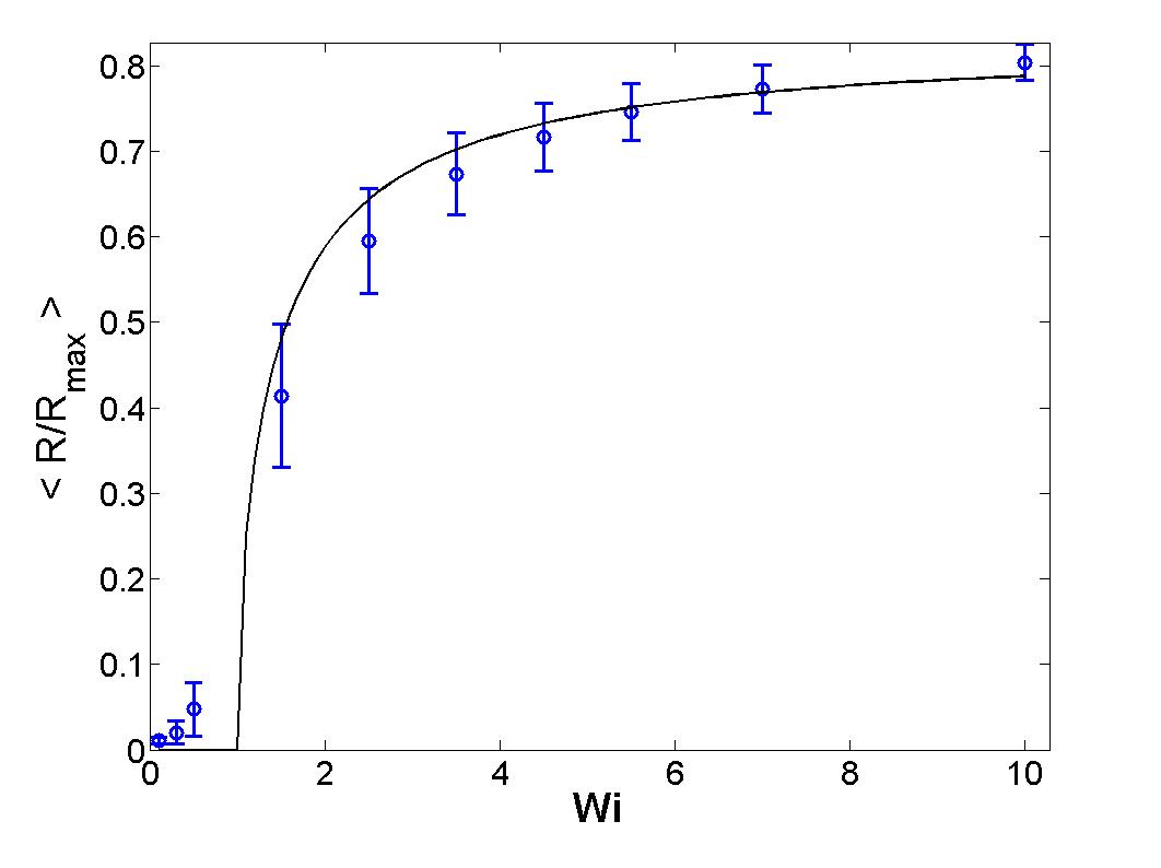
Figure 8: (Color online) The mean of normalized polymer extensions $\left\langle R/R_{\rm max}\right\rangle$ as a function of Weissenberg number Wi. The mean is calculated over the whole channel and the standard deviation is shown as error bar. The continuous line is the right hand side of (21) calculated for $\mbox{Wi}>1$.

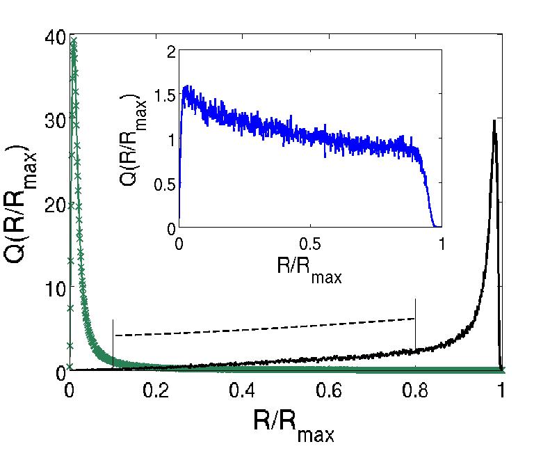
Figure 9: (Color online) The PDF of polymer extensions $Q(R)$ as a function of $R$ for different Wi showing the coil-stretch transition. The line with $(\times)$ symbols is for $\mbox{Wi}=0.5$ ($\tau_{\rm poly}=5$), the continuous line is for $\mbox{Wi}=10$ ($\tau_{\rm poly}=100$) and the inset is for $\mbox{Wi}=1.5$ ($\tau_{\rm poly}=15$). The PDF for $\mbox{Wi}=10$ is multiplied by $2$ to make it clear in the same scale. The dashed line shows power-law scaling with exponent $\alpha=1.48$.

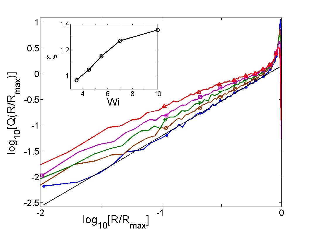
Figure 10: (Color online) Log-log plot of the PDF of polymer extensions for $\mbox{Wi}=3.5(\vartriangle),4.5(\square),5.5(+),7(\circ),10(\bullet)$. The straight line is a fit to the PDF for $\mbox{Wi}=10$. Similar fits yield the exponents $\zeta$ which are plotted as a function of Wi in the inset.

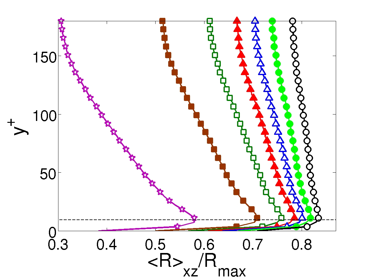
Figure 11: (Color online) The average polymer extensions $\left\langle R\right\rangle_{xz}$ as a function of the wall-normal coordinate $y^{+}$ for different Weissenberg numbers, v.i.z., $\mbox{Wi}=1.5(\star),2.5(\blacksquare),3.5(\square),4.5(\blacktriangle),5.5(\vartriangle),7($•$),10(\circ).$ The maximum occurs at $y^{+}\approx 10$.

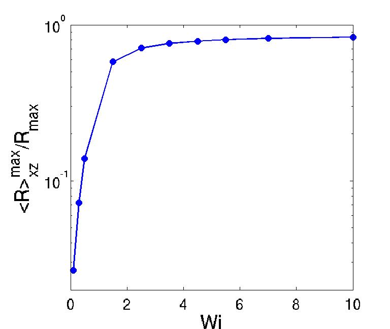
Figure 12: (Color online) The maxima of the average polymer extensions $\left\langle R\right\rangle_{xz}$ across the channel as a function of Wi in semilog scale.

III.4 Statistics of polymer orientation

In this section we present the results related to the orientation of the polymers. First let us discuss the orientation of the polymers with respect to the geometry of the channel. Let us denote the unit vector along ${\bm{R}}$ to be ${\bm{e}}$. The PDF of the three components of ${\bm{e}}$, $e_{x}$, $e_{y}$ and $e_{z}$, (i.e., three direction cosines of ${\bm{R}}$) are plotted in Fig. (13a) for polymers close to the wall ($y^{+}\approx 7$) and for three different values of Wi. For $\mbox{Wi}<1$ , i.e., below the coil-stretch transition the polymers are almost equally probable to point in any direction or in other words as the polymers are coiled as a sphere no preferential direction is selected. Above the coil-stretch transition polymers close to the wall have a high probability of being oriented along the $x$ axis, which is the stream-wise direction. This trend has been observed earlier in Ref. gup+sur+kho04 . A similar plot for polymers close to the center line ($y^{+}\approx 180$) is given in Fig. (13b). For small Wi all directions are equally probable. But as Wi increases here too the polymers get preferentially oriented along the stream-wise direction although the trend is much weaker than near the wall.

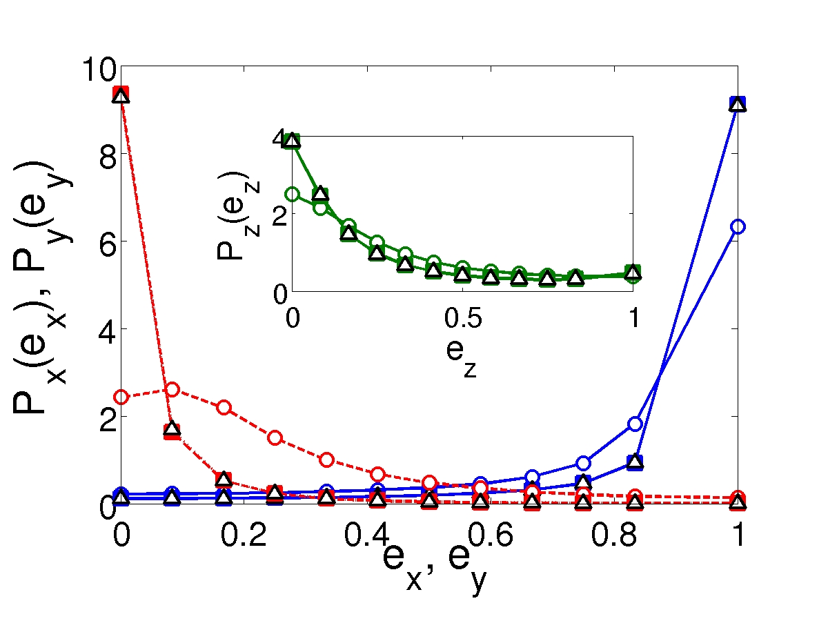
Figure 13: (Color online) PDF of the three direction cosines of polymer end-to-end separation vector ${\bm{R}}$ (a) for polymers near the wall and (b) for polymers at the center of the channel. Three different values of Wi are used. Namely, $\mbox{Wi}=0.1(\circ),1.5(\vartriangle),4.5(\blacksquare)$. The data for $\mbox{Wi}=1.5$ and $4.5$ coincide on each other. The PDFs of $e_{x}$ and $e_{y}$ are respectively plotted using continuous line with symbols ($P_{\rm x}$) and dashed lines with symbols ($P_{\rm y}$). The inset shows the PDF of $e_{z}$, $P_{\rm z}$.

We have also investigated the orientation of the polymers with respect to the three principal directions of the rate of strain tensor. For this purpose we first determine the three real eigenvalues of the symmetric rate of strain tensor and order them such that $\lambda_{1}>\lambda_{2}>\lambda_{3}$. We denote the components of the unit vector ${\bm{e}}$ (which is the unit vector along ${\bm{R}}$) along these three perpendicular directions by $e_{1}$, $e_{2}$ and $e_{3}$; these are merely the cosines of the angles between ${\bm{R}}$ and the three principal directions of the strain tensor. The PDFs of $e_{1}$, $e_{2}$ and $e_{3}$ are plotted in the Fig. (14a) for polymers close to the wall ($y^{+}\approx 7$) and for three different values of Wi. The peak seen in Fig. (14) corresponds to the polymers orientating along the stream-wise direction as shown already in Fig. (13). Interestingly the polymers are not preferentially oriented along the strongest direction of strain $\lambda_{1}$ but along the stream-wise direction. This has an angle of about 45 degrees with respect to the x-axis since the main component of the strain rate comes from the wall-normal shear $\partial U/\partial y$.

Close to the centerline however the PDFs look quite different [Fig. (14b)]. For small Wi there is no preferential orientation but as Wi increases the polymers develops a trend of orienting parallel to the direction of either $\lambda_{1}$ or $\lambda_{2}$ and shows anti-alignment to $\lambda_{3}$.

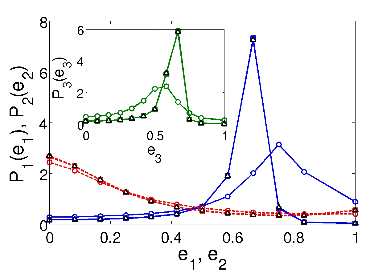
Figure 14: (Color online) PDF of $e_{1}$, $e_{2}$ and $e_{3}$, components of the unit vector along ${\bm{R}}$ along the three principal directions of strain: (a) for polymers near the wall, and (b) for polymers near the centerline. Three different Wi are used. Namely, $\mbox{Wi}=0.1(\circ),1.5(\vartriangle),4.5(\blacksquare)$. The data for $\mbox{Wi}=1.5$ and $4.5$ coincide on each other. The PDFs of $e_{1}$ and $e_{2}$ are respectively plotted using continuous line with symbols ($P_{\rm 1}$) and dashed line with symbols ($P_{\rm 2}$). The inset shows the PDF of $e_{3}$, $P_{\rm 3}$.

Finally we look at the relative orientation between the polymer end-to-end vector ${\bm{R}}$ and the vorticity vector ${\bm{\omega}}$. Close to the wall we find that PDF of the cosine of the angle $\psi$ between ${\bm{R}}$ and ${\bm{\omega}}$ has a peak at zero, see Fig. (15a). This implies that the polymers show a weak tendency to lie in the plane perpendicular to ${\bm{\omega}}$. However this trend is reversed near the centerline Fig. (15b) where the polymers orient along the vorticity vector.

To summarize the polymers near the wall shows the cleanest trend in their orientation. They show a strong tendency to line along the stream-wise directions. Weaker trends are seen near the center. The statistics of orientation of polymers near the center of our flow is very similar to the statistics of orientation of polymers obtained in homogeneous and isotropic flows wat+got10 . Note however that the orientation effects are much stronger near the wall than near the centerline.

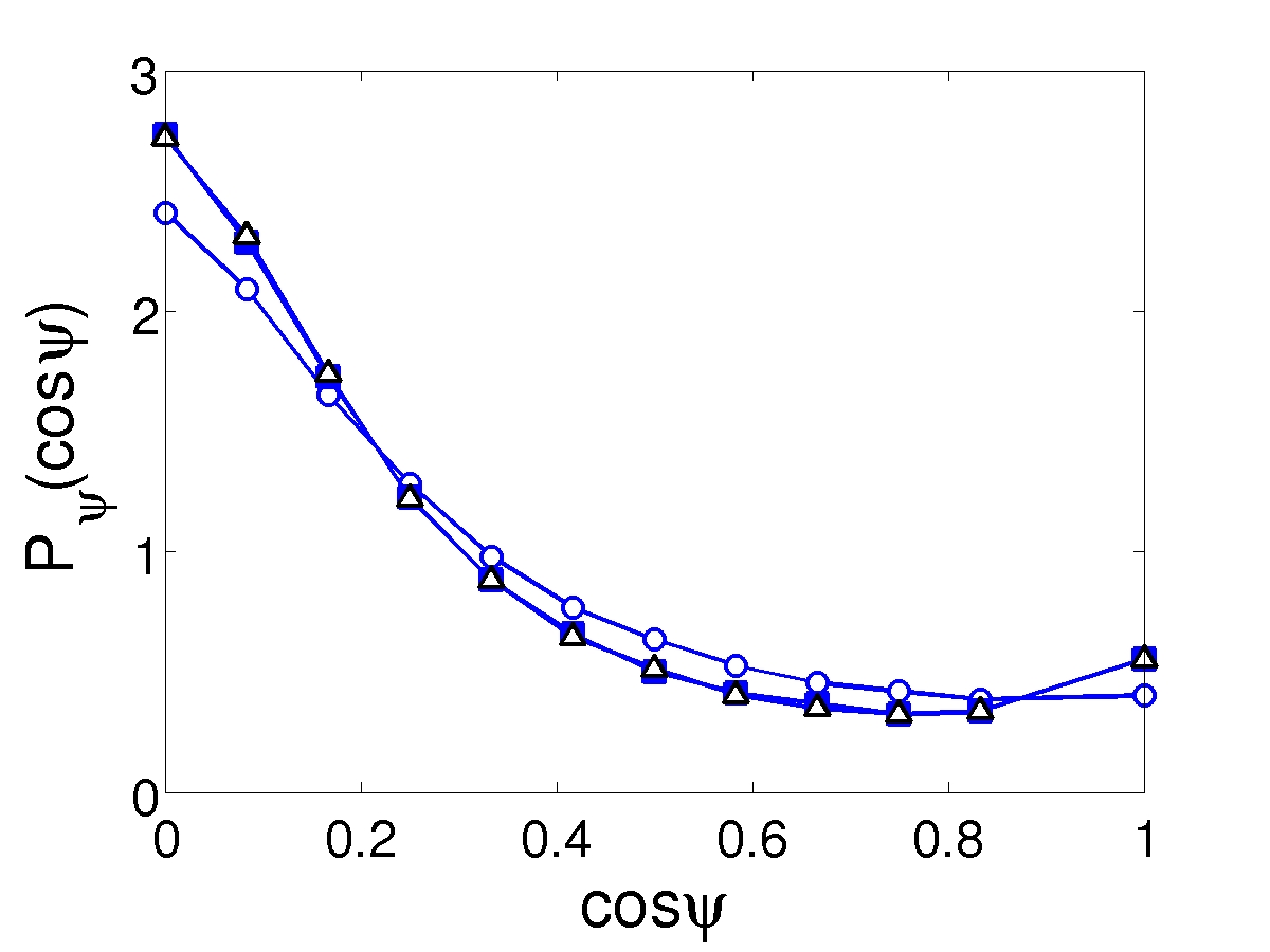
Figure 15: (Color online) PDF of $\cos(\psi)$, where $\psi$ is the angle between the polymer end-to-end vector ${\bf R}$ and vorticity, (a) for polymers near the wall and (b) for polymers near the centerline. Three different valus of Wi are plotted. Namely $\mbox{Wi}=0.1(\circ)$, $1.5(\vartriangle)$, $4.5(\blacksquare)$.

IV Conclusions

We have presented in this paper an extensive numerical study of the passive Lagrangian polymers in turbulent channel flow. We have used both linear (Oldroyd-B) and nonlinear (FENE) polymers. To understand the statistics of polymer end-to-end vector it is necessary to know the statistics of the Finite Time Lyapunov Exponents. For this purpose in addition to the polymers we have solved the equation of evolution of infinitismal line elements in the turbulent flow and calculated the FTLEs for an inhomogeneous flow. We find that the PDF of FTLEs does admit a large deviation expression, and we calculate a corresponding Cramer’s function. Note, however, that the large deviation expression is valid only at very large times. In addition we use the location of the minima of the Cramer’s function to define our Weissenberg number. Consequently for the FENE model we observe coil-stretch transition at $\mbox{Wi}\approx 1$. For the Oldroyd-B model we find that the PDF of polymer extension shows power-law behavior for $\mbox{Wi}<1$. We calculate the exponent of this power-law using the rank-order method. We also calculate the same exponent from the Cramer’s function using the theory of Ref. bal+fux+leb00 . These two different calculations match within error, validating the theory of Ref bal+fux+leb00 . This shows that the idealizations used in Ref. bal+fux+leb00 , in particular the assumption that in Lagrangian coordinates the rate-of-strain tensor $\sigma_{\alpha\beta}$ is delta-correlated in time is a reasonable approximation at least for linear polymers below the coil-stretch transition even in the case of a realistic flow. For the FENE model we cannot meaningfully calculate the PDF of polymer extension from the Cramer’s function using the results of Ref. che00 because our numerically calculated Cramer’s function is not accurate enough for this exercise. For the FENE model we find that the polymers are more extended near the wall, but the difference decreases as Weissenberg number increases far beyond the coil-stretch transition. We further find that near the center of the channel the orientational statistics of the polymers show similarity to orientational statistics obtained for homogeneous and isotropic flows wat+got10 ,i.e., they align along either of the two largest directions of strain and tend to orient orthogonal to the third principal direction of strain. A much stronger orientational trend is seen near the wall where the orientations of the polymers are along the stream-wise direction.

Although our DNSs involve passive polymers it is possible to have insights on polymeric drag reductions from these simulations. We can calculate the polymeric stress from our simulations and add this to the Reynolds stresses to see how they change the Reynolds-averaged flow equations. It would be interesting to see how much of drag-reduction can be described by this simple approach. Such results will be presented in a future publication.

V Acknowledgements

We thank A. Brandenburg, O. Flores, V. Steinberg, A. Vulpiani, and D. Vincenzi for helpful discussions. Financial support from the Swedish Research Council under the grant 2011-5423 and computer time provided by SNIC (Swedish National Infrastructure for Computing) are gratefully acknowledged.

References

- (1) B. Toms, in Proceedings of First International Congress on Rheology (North-Holland, Amsterdam, 1949), pp. Section II, 135.
- (2) T. Squires and S. Quake, Rev. Mod. Phys. 77, 977 (2005).
- (3) J. Lumley, J. Polymer Sci 7, 263 (1973).
- (4) E. Hinch, Phys. Fluids. 20, S22 (1977).
- (5) J.M. Deutsch, Phys. Rev. Lett. 69, 1536 (1992).
- (6) E. Balkovsky, A. Fouxon, and V. Lebedev, Phys. Rev. Lett. 84, 4765 (2000).
- (7) M. Chertkov, Phys. Rev. Lett. 84, 4761 (2000).
- (8) J. Thiffeault, Physics Letters A 308, 445 (2003).
- (9) M.M. Afonso and D. Vincenzi, Journal of Fluid Mechanics 540, 99 (2005).
- (10) K. Turitsyn, Journal of Experimental and Theoritical Physics 105, 655 (2007).
- (11) H. Massah, K. Kontomaris, W.R. Schowalter, and T.J. Hanratty, Phys. Fluids. A 5, 881 (1993).
- (12) S. Musacchio and D. Vincenzi, J. Fluid Mech. 670, 326 (2011).
- (13) A. Celani, A. Puliafito, and K. Turitsyn, Europhysics Letters 70, 464 (2005).
- (14) M. Chertkov, I. Kolokolov, V. Lebedev, and K. Turitsyn, Journal of Fluid Mechanics 531, 251 (2005).
- (15) P.A. Stone and M.D. Graham, Physics of Fluids 15, 1247 (2003).
- (16) B. Eckhardt, J. Kronjäger, and J. Schumacher, Comp. Physics Comm. 147, 538 (2002).
- (17) V.K. Gupta, R. Sureshkumar, and B. Khomami, Phys. Fluids. 16, 1546 (2004).
- (18) T. Watanabe and T. Gotoh, Phys. Rev. E 81, 066301 (2010).
- (19) G. Boffetta, A. Celani, and S. Musacchio, Phys. Rev. Lett 91, 034501 (2003).
- (20) A. Gupta, P. Perlekar, and R. Pandit, ArXiv:1207.4774 (2012).
- (21) P. Perlekar, D. Mitra, and R. Pandit, Phys. Rev. Lett. 97, 264501 (2006).
- (22) P. Perlekar, D. Mitra, and R. Pandit, Phys. Rev. E 82, 066313 (2010).
- (23) V. Dallas, J. C. Vassilicos, and G. F. Hewitt, Phys. Rev. E 82, 066303 (2010).
- (24) Y. Dubief et al., J. Fluid. Mech 514, 271 (2004).
- (25) V. Terrapon, Ph.D. thesis, Department of Mechanical Engineering, Stanford University., 2005.
- (26) T. Peters and J. Schumacher, Phys. Fluids 19, 065109 (2007).
- (27) G. Falkovich, K. Gawȩdzki, and M. Vergassola, Rev. Mod. Phys. 73, 913 (2001).
- (28) B. Eckhardt, E. Hascoët, and W. Braun, in Proceedings ”IUTAM Symposium on Nonlinear Stochastic Dynamics”, edited by N. S. Namachchivaya and Y. K. Lin (Springer, Berlin, 2002), pp. 990–999.
- (29) K. Gawedzki, ArXiv:0806.1949 (2008).
- (30) S. Jin and L. R. Collins, New J. Phys. 9, 360 (2007).
- (31) A. Monin and A. Yaglom, STATISTICAL FLUID MECHANICS: Mechanics of Turbulence, volume 1 (Dover Publications, Inc, Mineola, New York, 2007).
- (32) M. Chevalier, P. Schlatter, A. Lundbladh, and D. Henningson, SIMSON: A pseudospectral solver for incompressible boundary layer flows., Mekanik, Kungliga Tekniska högskolan, 2007.
- (33) R. Moser, J. Kim, and N. Mansour, Physics of Fluids 11, 943 (1999).
- (34) F. Bagheri, Master’s thesis, KTH, School of Engineering Sciences (SCI), Mechanics, 2010.
- (35) G. Sardina et al., J. Fluid Mech. 699, 50 (2012).
- (36) J. Jeong, F. Hussain, W. Schoppa, and J. Kim, J. Fluid Mech. 332, 185 (1997).
- (37) R. Bird, C. Curtiss, R. Armstrong, and O. Hassager, Dynamics of Polymeric Liquids (Wiley, New York, 1987).
- (38) N. Phan-Thien, Understanding Viscoelasticity (Springer, Berlin, 2002).
- (39) D. Higham, SIAM Review 43, 525 (2001).
- (40) T. Vaithianathan and L. Collins, Journal of Computational Physics 187, 1 (2003).
- (41) T. Vaithianathann, A. Robert, J. Brasseur, and L. Collins, J. Non-newtonian Fluid Mech. 140, 3 (2006).
- (42) P. Perlekar, Ph.D. thesis, Indian Institute of Science, Bangalore, India, 2009.
- (43) R. Benzi, E. De Angelis, R. Govindarajan, and I. Procaccia, Phys. Rev. E 68, 016308 (2003).
- (44) E. D. angelis, C. Casciola, R. Benzi, and R. Piva, J. Fluid. Mech 531, 1 (2005).
- (45) J. Bec et al., Phys. Fluids 18, 091702 (2006).
- (46) J. Kurths and A. Brandenburg, Phys. Rev. A 44, R3427 (1991).
- (47) D. Mitra, J. Bec, R. Pandit, and U. Frisch, Phys. Rev. Lett 94, 194501 (2005).
- (48) Y. Liu and V. Steinberg, Euro. Phys. Lett. 90, 44005 (2010).
- (49) White and Mungal, Annual Review of Fluid Mechanics 40, 235 (2008).