Induced subgraphs in sparse random graphs with given degree sequence

Abstract

Let $\mathcal{G}_{n,d}$ denote the uniformly random $d$-regular graph on $n$ vertices. For any $S\subset[n]$, we obtain estimates of the probability that the subgraph of $\mathcal{G}_{n,d}$ induced by $S$ is a given graph $H$. The estimate gives an asymptotic formula for any $d=o(n^{1/3})$, provided that $H$ does not contain almost all the edges of the random graph. The result is further extended to the probability space of random graphs with a given degree sequence.

1 Introduction

Properties of subgraphs and induced subgraphs in random graph models have been investigated by various authors. Ruciński [12, 14] studied the distribution of the count of small subgraphs in the standard random graph model $\mathcal{G}_{n,p}$, and conditions under which the distribution converges to the normal distribution. He also studied properties of induced subgraphs in [13].

Techniques for analysing the standard random graph model $\mathcal{G}_{n,p}$ often do not apply in the random regular graph model $\mathcal{G}_{n,d}$. We take the vertex set of the graph to be $[n]$ in both these models. For $S\subseteq[n]$, let $G_{S}$ denote the subgraph of $G$ induced by $S$. For a graph $H$ with vertex set $S$, computing the probabilities ${\bf P}(G_{S}\supseteq H)$ and ${\bf P}(G_{S}=H)$ in $\mathcal{G}_{n,p}$ is trivial, but computing them in $\mathcal{G}_{n,d}$ is not easy, especially when the degree $d\to\infty$ as $n\to\infty$. McKay [8] estimated lower and upper bounds of ${\bf P}(G_{S}\supseteq H)$ in $\mathcal{G}_{n,d}$ when the degree sequence of $H$ and $d$ satisfy certain conditions. These bounds are useful in estimating the asymptotic value of ${\bf P}(G_{S}\supseteq H)$ when $d$ is not too large or $H$ is small. Z. Gao and the third author [6] proved that the distribution of the number of small subgraphs with certain restrictions (such as $d$ not growing too quickly) converges to the normal distribution in $\mathcal{G}_{n,d}$. No such results on induced subgraphs have been derived, although the main results of [8] could be used as a basis for obtaining results on induced subgraphs. However, this would require severe restrictions on the size of the subgraphs, and seems unlikely to apply to subgraphs with more than $n^{2/3}$ vertices for any $d$.

On the other hand, for very dense regular graphs, Krivelevich, Sudakov and Wormald [7] computed ${\bf P}(G_{S}=H)$ in $\mathcal{G}_{n,d}$ when $n$ is odd, $d=(n-1)/2$ and $|V(H)|=o(\sqrt{n})$. McKay [11] has recently given a stronger result, for more general degree sequences and provided $H$ has less than $n^{1+\epsilon}$ edges for some $\epsilon>0$.

An asymptotic formula of the probability that $G_{S}=H$ or $G_{S}\supseteq H$ in a random bipartite graph with a specified degree sequence has been derived by Bender [2] when the maximum degree is bounded. The result was extended further by Bollobás and McKay [4] and by McKay [9] when the maximum degree goes to infinity slowly as $n$ goes to infinity. Greenhill and Mckay [5] recently derived an asymptotic formula for the case when the random bipartite graph is sufficiently dense and $H$ is sparse enough.

For a vector ${\bf d}=(d_{1},\ldots,d_{n})$ of nonnegative integers, let $M=M({\bf d})=\sum_{i=1}^{n}d_{i}$ and let $\mathcal{G}_{{\bf d}}$ denote the class of graphs with degree sequence ${\bf d}$ and the uniform distribution (so $\mathcal{G}_{{\bf d}}$ is a generalisation of $\mathcal{G}_{n,d}$). In this paper, we compute the probability that $G_{S}=H$ in $\mathcal{G}_{{\bf d}}$ when $d_{\max}=o((M-2m(H))^{1/4})$, where $m(H)$ denotes the number of edges in $H$ and $d_{\max}=\max\{d_{1},\ldots,d_{n}\}$. The power of this result is that there is no major restriction on the size or density of $H$. In Section 2, as a direct application of our main result, we compute the probability that a given set of vertices in $\mathcal{G}_{n,d}$ is an independent set. Our results will also be useful as a basic tool for studying the properties of induced subgraphs in the binomial random graph ${\mathcal{G}}(n,p)$, such as the subgraph induced by the vertices of even degree, or odd degree.

A graph $G$ is called a B-graph with vertex bipartition $(L,R)$ if $V(G)=L\cup R$, and $L$ is an independent set of $G$. If the graph is not necessarily simple, i.e. loops and multiple edges are allowed, we call it a B-multigraph instead. An edge in a B-graph or B-multigraph is called a mixed edge if its end vertices are in $L$ and $R$ respectively, and a pure edge if they are both in $R$. Given a nonnegative integer vector ${\bf d}$, let $\mathcal{G}(L,R,{\bf d})$ be the set of B-graphs with bipartition $L$ and $R$ and the degree sequence ${\bf d}$ and let $g(L,R,{\bf d})=|\mathcal{G}(L,R,{\bf d})|$. By convention, $g(L,R,{\bf d})=0$ if ${\bf d}$ is not nonnegative.

Given a sequence ${\bf d}$, let $g({\bf d})$ denote the number of graphs on vertex set $[n]$ with degree sequence ${\bf d}$. Given $S=[s]\subset[n]$, let $H$ be a given graph on vertex set $S$ with degree sequence $(k_{i})_{1\leq i\leq s}$. Let $\bf{d^{\prime}}$ be the integer vector defined by $d^{\prime}_{i}=d_{i}-k_{i}$ for $i\in S$ and $d^{\prime}_{i}=d_{i}$ for $i\in[n]\setminus S$. Then the number of graphs with degree sequence ${\bf d}$ and with $G_{S}=H$ is $g(S,[n]\setminus S,{\bf d^{\prime}})$, and so the probability that $G_{S}=H$ in $\mathcal{G}_{n,{\bf d}}$ equals $g(S,[n]\setminus S,{\bf d^{\prime}})/g({\bf d})$. So the study of induced subgraphs leads directly to the question of counting B-graphs.

The following theorem by McKay [9] gives an asymptotic formula for $g({\bf d})$ when $d_{\max}^{4}=o(M({\bf d}))$. (The restriction on $d_{\max}$ was relaxed further by McKay and Wormald in [10], but to do so requires a few extra terms in the exponential factor of the asymptotic formula, and is not needed for the purpose of this paper.)

Theorem 1.1 (McKay)

Let ${\bf d}=(d_{1},\ldots,d_{n})$ with $\sum_{i=1}^{n}d_{i}$ even and $d_{\max}=o(M({\bf d})^{1/4})$. The number of graphs with degree sequence $\bf d$ is uniformly

$$\frac{M({\bf d})!}{2^{M({\bf d})/2}(M({\bf d})/2)!\prod_{i=1}^{n}d_{i}!}\cdot\exp\left(-\mu({\bf d})-\mu({\bf d})^{2}+O(d_{\max}^{4}/M({\bf d}))\right)$$

as $n\to\infty$.

By “uniformly” in the above theorem we mean the constant implicit in $O(.)$ is the same for all choices of ${\bf d}$ as a function of $n$, for a given function implicit in the $o(.)$ term. A special case of Theorem 1.1 gives that the number of $d$-regular graphs on $n$ vertices is asymptotically

$$\frac{(dn)!}{2^{dn/2}(dn/2)!(d!)^{n}}\cdot\exp\left(-\frac{d^{2}-1}{4}\right),$$

when $d=o(n^{1/3})$.

Our main result is an asymptotic formula for $g(L,R,{\bf d})$, to an accuracy matching McKay’s formula in Theorem 1.1. This is given in Section 2, together with its direct applications to estimating ${\bf P}(G_{S}=H)$ in $\mathcal{G}_{{\bf d}}$, and some special cases are also given there. The proofs use the switching method, first introduced by McKay [9], with refinements by McKay and Wormald [10], and suitably modified for our purposes here. In Section 3 we use switchings to estimate the ratios between probabilities defined by the counts of loops and various types of multiple edges. In Section 4 we again use switchings to evaluate some variables appearing in those estimates, and in Section 5 we use these to prove the main theorem.

2 Main results

Our main goal in this paper is to estimate $g(L,R,{\bf d})$. We first define some notation. For any positive integer $n$, let $[n]$ denote the set $\{1,2,\ldots,n\}$. Given a sequence ${\bf d}=(d_{1},\ldots,d_{n})$, let $d_{\max}=\max\{d_{i},i\in[n]\}$ and let $M_{2}({\bf d})=\sum_{i=1}^{n}d_{i}(d_{i}-1)$. Define $\mu({\bf d})$ to be $M_{2}({\bf d})/2M({\bf d})$.

For any $S\subset L\cup R$, define

$$M_{1}({\bf d},S)=\sum_{i\in S}d_{i},\quad M_{2}({\bf d},S)=\sum_{i\in S}d_{i}(d_{i}-1),$$

$$\mu_{0}({\bf d},L,R) = \frac{(M_{1}({\bf d},R)-M_{1}({\bf d},L))M_{2}({\bf d},R)}{2M_{1}({\bf d},R)^{2}},$$ (2.1)

$$\mu_{1}({\bf d},L,R) = \frac{M_{2}({\bf d},R)M_{2}({\bf d},L)}{2M_{1}({\bf d},R)^{2}},$$ (2.2)

$$\mu_{2}({\bf d},L,R) = \mu_{0}({\bf d},L,R)^{2}.$$ (2.3)

We drop the notations $L$ and $R$ from $\mu_{i}({\bf d},L,R)$ for $i=0,1,2$ when the context is clear. Note also that if $M_{1}({\bf d},R)<M_{1}({\bf d},L)$, then $g(L,R,{\bf d})$ is trivially $0$, so we may assume that

$$M_{1}({\bf d},R)\geq M_{1}({\bf d},L).$$ (2.4)

The following theorem, proved in Section 5, gives an asymptotic formula for $g(L,R,\bf{d})$.

Theorem 2.1

Let ${\bf d}=(d_{1},\ldots,d_{n})$ with $\sum_{i=1}^{n}d_{i}$ even, $d_{\max}=o(M({\bf d})^{1/4})$ and $M_{1}({\bf d},R)\geq M_{1}({\bf d},L)$. Then uniformly over all $L$ and ${\bf d}$ as $n\to\infty$,

$$g(L,R,{\bf d}) = \frac{M_{1}({\bf d},R)!e^{-\mu_{0}({\bf d})-\mu_{1}({\bf d})-\mu_{2}({\bf d})}}{2^{(M_{1}({\bf d},R)-M_{1}({\bf d},L))/2}((M_{1}({\bf d},R)-M_{1}({\bf d},L))/2)!\prod_{i=1}^{n}d_{i}!}\left(1+O\left(\frac{d_{\max}^{4}}{M({\bf d})}\right)\right).$$

Applying Theorems 2.1 and 1.1 we directly get the following. Here $d^{\prime}_{\max}$ denotes $\max\{d_{1}^{\prime},\ldots,d_{n}^{\prime}\}$.

Corollary 2.2

Let ${\bf d}=(d_{1},\ldots,d_{n})$ with $\sum_{i=1}^{n}d_{i}$ even and $d_{\max}=o(M({\bf d})^{1/4})$. Let $S=[s]\subset[n]$, let $H$ be a graph on vertex set $S$ with degree sequence ${\bf k}=(k_{1},\ldots,k_{s})$, let $h=\sum_{i=1}^{h}k_{i}$ and let ${\bf d}^{\prime}=(d^{\prime}_{1},\ldots,d^{\prime}_{n})$ with $d^{\prime}_{i}=d_{i}-k_{i}$ for $i\in S$ and $d^{\prime}_{i}=d_{i}$ for $i\notin S$. If $d^{\prime}_{i}<0$ for some $i\in[n]$ or $M_{1}({\bf d}^{\prime},[n]\setminus S)<M_{1}({\bf d}^{\prime},S)$, then ${\bf P}_{\mathcal{G}_{{\bf d}}}(S,H)=0$. Otherwise, if $d^{\prime}_{\max}=o(M({\bf d^{\prime}})^{1/4})$, then uniformly

$${\bf P}_{\mathcal{G}_{{\bf d}}}(S,H) = \exp\left(-\mu_{0}({\bf d}^{\prime})-\mu_{1}({\bf d}^{\prime})-\mu_{2}({\bf d}^{\prime})+\mu({\bf d})+\mu({\bf d})^{2}+O\left(\frac{{d^{\prime}}_{\max}^{4}}{M({\bf d^{\prime}})}+\frac{d_{\max}^{4}}{M({\bf d})}\right)\right)$$

$$\times\prod_{i=1}^{s}[d_{i}]_{k_{i}}\frac{M_{1}({\bf d}^{\prime},[n]\setminus S)!2^{M_{1}({\bf d}^{\prime},S)+h/2}(M({\bf d})/2)!}{((M_{1}({\bf d}^{\prime},[n]\setminus S)-M_{1}({\bf d}^{\prime},S))/2)!M({\bf d})!}.$$

where $\mu_{i}({\bf d}^{\prime})=\mu_{i}({\bf d}^{\prime},S,[n]\setminus S)$ for $i=0$, $1$ and $2$.

Proof.  Recall that $g({\bf d})$ denote the number of graphs on vertex set $[n]$ with degree sequence ${\bf d}$. We have

$${\bf P}_{\mathcal{G}_{{\bf d}}}(S,H)=\frac{g(S,[n]\setminus S,{\bf d^{\prime}})}{g({\bf d})}.$$

The corollary now follows from the formulae for $g(S,[n]\setminus S,{\bf d^{\prime}})$ in Theorem 2.1 and $g({\bf d})$ in Theorem 1.1.    

Let ${\bf P}_{\mathcal{G}_{n,d}}(S,H)$ denote the probability that $G_{S}=H$ for a random $d$-regular graph $G$.

Corollary 2.3

Given $0<s<n$, let $S=[s]\subset[n]$, let $H$ be a graph on vertex set $S$ with degree sequence ${\bf k}=(k_{1},\ldots,k_{s})$ with $k_{i}\leq d$ for all $1\leq i\leq s$, and put $h=\sum_{i=1}^{h}k_{i}$. Assume $d=o((n-s)^{1/3})$. Then

$${\bf P}_{\mathcal{G}_{n,d}}(S,H) = \exp\left(-\mu_{0}({\bf d}^{\prime})-\mu_{1}({\bf d}^{\prime})-\mu_{2}({\bf d}^{\prime})+\frac{d^{2}-1}{4}+O(d^{4}/(dn-h))\right)$$

$$\hskip 14.22636pt\times\prod_{i=1}^{s}[d]_{k_{i}}\frac{(dn-ds)!(dn/2)!2^{ds-h/2}}{((dn-2ds+h)/2)!(dn)!}\,,$$

where $d^{\prime}_{i}=d-k_{i}$ for $i\in S$ and $d^{\prime}_{i}=d$ for $i\notin S$, and $\mu_{i}$ is defined as in Corollary 2.2.

Proof.  We apply Corollary 2.2. By the definition of $\mu(\bf d)$, we immediately get that $\mu({\bf d})+\mu({\bf d})^{2}=(d^{2}-1)/4$ when ${\bf d}$ is a constant sequence with each term $d$. We also have $M({\bf d})=dn$, $M({\bf d}^{\prime})=dn-h$, $M_{1}({\bf d}^{\prime},S)=ds-h$, $M_{1}({\bf d}^{\prime},[n]\setminus S)=dn-ds$, and $d^{\prime}_{\max}\leq d$. Moreover,

$$\frac{(d_{\max}^{\prime})^{4}}{M({\bf d}^{\prime})}=\frac{d^{4}}{dn-h}=\frac{d^{3}}{n-h/d}\leq\frac{d^{3}}{n-s}=o(1),$$

since $h\leq ds$ and $d=o((n-s)^{1/3})$.    

The formula in Corollary 2.3 easily simplifies if the graph $H$ is not too large.

Corollary 2.4

Let $S$, $H$, ${\bf k}$ and $h$ be defined as in Corollary 2.3. If $d=o(n^{1/3})$, $s^{2}d=o(n)$ and $d^{2}s=o(n)$, then

$${\bf P}_{\mathcal{G}_{n,d}}(S,H)=\big{(}1+O((d^{3}+s^{2}d+d^{2}s)/n)\big{)}(dn)^{-h/2}\prod_{i=1}^{s}[d]_{k_{i}}.$$

Proof.  Since $d^{2}s=o(n)$, we have $h=O(ds)=o(n)$ and hence $d^{4}/(dn-h)=O(d^{3}/n).$ Similarly,

$$M_{1}({\bf d}^{\prime},R)=dn+O(ds),\quad M_{i}({\bf d}^{\prime},L)=O(d^{i}s)\ (i=1,2),\quad M_{2}({\bf d}^{\prime},R)=d(d-1)(n-O(s))$$

and hence from (2.1)–(2.3),

$$\mu_{0}({\bf d^{\prime}})=\frac{d-1}{2}+O(ds/n),\quad\mu_{1}({\bf d^{\prime}})=O\left(d^{2}s/n\right),\quad\mu_{2}({\bf d^{\prime}})=\frac{(d-1)^{2}}{4}+O(d^{2}s/n).$$

Thus $\mu_{0}({\bf d^{\prime}})+\mu_{1}({\bf d^{\prime}})+\mu_{2}({\bf d^{\prime}})=(d^{2}-1)/4+O(d^{2}s/n)$.

The corollary now follows upon applying Stirling’s formula in the form $n!=\sqrt{2\pi n}(n/e)^{n}(1+O(n^{-1}))$ to obtain (ignoring negligible error terms)

$$\frac{(dn-ds)!(dn/2)!2^{ds-h/2}}{((dn-2ds+h)/2)!(dn)!}=\left(\frac{dn}{e}\right)^{-h/2}\frac{(1-s/n)^{dn-ds}}{(1-2s/n+h/dn)^{(dn-2ds+h)/2}}.~{}~{}\vrule height=8.0pt,width=4.0pt,depth=0.0pt$$

Another interesting special case is when $H$ is empty.

Corollary 2.5

Assume $d=o(n^{1/3})$. Then for any $S\subset[n]$ with $s=|S|<n/2$,

$${\bf P}(S\ \mbox{is independent})=\big{(}1+O(d^{3}/n)\big{)}\exp\left(f(d,\delta)\right)\prod_{i=1}^{s}\frac{(dn-ds)!(dn/2)!2^{ds}}{((dn-2ds)/2)!(dn)!},$$

where $\delta=\delta(n)=s/n$, and

$$f(d,\delta)=-\frac{\delta(d-1)(\delta d-2+\delta)}{4(1-\delta)^{2}}.$$

Proof.  This is a simple application of Corollary 2.3 with $h=0$, noting that

$$\mu_{0}=\frac{(d-1)(n-2s)}{2(n-s)},\ \mu_{1}=\frac{(d-1)^{2}s}{2(n-s)},\ \mu_{2}=\frac{(d-1)^{2}(n-2s)^{2}}{4(n-s)^{2}}.~{}~{}\vrule height=8.0pt,width=4.0pt,depth=0.0pt$$

Note that if $d(n-2s)\to\infty$, then the probability that $S$ is independent under the conditions in Corollary 2.5 can be further simplified using Stirling’s formula to

$$\big{(}1+O(d^{3}/n)+O(1/(dn-2ds))\big{)}\sqrt{\frac{1-\delta}{1-2\delta}}\left(\frac{(1-\delta)^{1-\delta}}{(1-2\delta)^{(1-2\delta)/2}}\right)^{dn}\exp\left(f(d,\delta)\right).$$

3 The main switchings

We can use the pairing model to generate B-graphs with the vertex partition $L\cup R$ and the degree sequence ${\bf d}=\{d_{1},\ldots,d_{n}\}$. Consider $n$ buckets representing the $n$ vertices. Let each bucket $i$ contain $d_{i}$ points. Take a random pairing of these points. We say a pairing is restricted if no pair has both ends in the buckets representing vertices in $L$. Let $\mathcal{M}(L,R,{\bf d})$ be the class of all restricted pairings. Every such pairing corresponds to a B-multigraph by contracting all points in each bucket to form a vertex. In the rest of the paper, a bucket in a pairing is also called a vertex. A pair in a pairing is called a mixed (pure) pair if it corresponds to a mixed (pure) edge in the corresponding B-multigraph. Thus, in a restricted pairing, each pair is either mixed or pure; pure pairs have both points in a vertex in $R$. Note that any simple B-graph corresponds to $\prod_{i=1}^{n}d_{i}!$ restricted pairings in $\mathcal{M}(L,R,{\bf d})$. Hence, all simple B-graphs occur with the same probability in the pairing model.

The main goal of this section is to compute the probability that a B-multigraph generated by the pairing model is simple. We say that $\{\{u_{1},u^{\prime}_{1}\},\{u_{2},u^{\prime}_{2}\},\{u_{3},u^{\prime}_{3}\}\}$ is a triple pair if $u_{1}$, $u_{2}$, $u_{3}$ are in one vertex and $u^{\prime}_{1}$, $u^{\prime}_{2}$, $u^{\prime}_{3}$ are in another vertex. We call the two vertices involved the end vertices of the triple pair. If the end vertices are in $L$ and $R$ respectively, the triple pair is called a mixed triple pair, and otherwise it is pure. Given a random restricted pairing, let $T_{1}$ and $T_{2}$ be the number of mixed and pure triple pairs respectively. In this section, there is only one degree sequence $\bf d$ referred to, so we drop the notation ${\bf d}$ from $M(\bf d)$ and $M_{i}({\bf d},L)$, $M_{i}({\bf d},R)$, $\mu_{i}({\bf d})$ for simplicity. Since $M_{1}(R)\geq M_{1}(L)$ by assumption (2.4), we have $M_{1}(R)\geq M/2$.

Lemma 3.1

${\bf E}(T_{1})=O(d_{\max}^{4}/M)$ and ${\bf E}(T_{2})=O(d_{\max}^{4}/M)$.

Proof.  For any two vertices $i\in L$ and $j\in R$, we compute the probability that there is a triple pair with end vertices $i$ and $j$. There are $\binom{d_{i}}{3}$ ways to choose three points from the vertex $i$ and $\binom{d_{j}}{3}$ ways to choose three points from the vertex $j$. There are $6$ ways to match the six chosen points to form a triple pair. For any positive even integer $m$, let $U(m)$ denote the number of pairings of $m$ points. Then

$$U(m)=\prod_{i=0}^{m/2-1}(m-2i-1)=\frac{m!}{2^{m/2}(m/2)!}.$$

The probability for the three particular pairs to occur is

$$\frac{[M_{1}(R)-3]_{M_{1}(L)-3}U(M_{1}(R)-M_{1}(L))}{[M_{1}(R)]_{M_{1}(L)}U(M_{1}(R)-M_{1}(L))}\sim M_{1}(R)^{-3}$$

(noting that $M_{1}(R)\geq M_{1}(L)$ implies $M_{1}(R)\to\infty$). This is because the number of ways to match the remaining $M_{1}(R)-3$ points in $L$ to points in $R$, except for the three chosen points in the vertex $j$, is $[M_{1}(R)-3]_{M_{1}(L)-3}$, and the number of matchings of the remaining $M_{1}(R)-M_{1}(L)$ points in $R$ is $U(M_{1}(R)-M_{1}(L))$, whilst the total number of restricted pairings is $[M_{1}(R)]_{M_{1}(L)}U(M_{1}(R)-M_{1}(L))$. Hence we have

$${\bf E}(T_{1}) \sim \sum_{i\in L}\sum_{j\in R}6\binom{d_{i}}{3}\binom{d_{j}}{3}M_{1}(R)^{-3}=O\left(\left(\sum_{i\in L}d_{i}^{3}\right)\left(\sum_{j\in R}d_{j}^{3}\right)\right)M^{-3}$$

$$= O\left(\frac{d_{\max}^{4}M_{1}(L)M_{1}(R)}{M^{3}}\right)=O\left(\frac{d_{\max}^{4}}{M}\right),$$

where the second equality uses $M/2\leq M_{1}(R)\leq M$.

A similar argument gives

$${\bf E}(T_{2}) \sim \sum_{i\in R}\sum_{j\in R}6\binom{d_{i}}{3}\binom{d_{j}}{3}M_{1}(R)^{-3}=O\left(\left(\sum_{i\in R}d_{i}^{3}\right)\left(\sum_{j\in R}d_{j}^{3}\right)\right)M^{-3}$$

$$= O\left(\frac{d_{\max}^{4}M_{1}(R)^{2}}{M^{3}}\right)=O\left(\frac{d_{\max}^{4}}{M}\right).~{}~{}\vrule height=8.0pt,width=4.0pt,depth=0.0pt$$

A pair $\{u,u^{\prime}\}$ is called a loop if $u$ and $u^{\prime}$ are contained in the same vertex and two pairs $\{u_{1},u^{\prime}_{1}\},\{u_{2},u^{\prime}_{2}\}$ are called a double pair if $u_{1}$, $u_{2}$ are in one vertex and $u^{\prime}_{1}$, $u^{\prime}_{2}$ are in another vertex. We call two loops that contain points from a common vertex a double loop. Let $I$ be the number of double loops. The proof of the following is a simple modification of the proof of the previous lemma, so is omitted.

Lemma 3.2

${\bf E}(I)=O(d_{\max}^{3}/M)$.    

Lemmas 3.1 and 3.2 show that a.a.s. there are no triple pairs or double loops in a random restricted pairing, under the assumption $d_{\max}^{4}=o(M({\bf d}))$. So we only need to consider loops and double pairs. In a restricted pairing, there are two types of double pairs. One is that $u_{1}$, $u_{2}$ are contained in a vertex in $L$ and $u^{\prime}_{1}$, $u^{\prime}_{2}$ are contained in a vertex in $R$. The other is that all of $u_{1}$, $u_{2}$, $u^{\prime}_{1}$ and $u^{\prime}_{2}$ are contained in vertices in $R$. We call the former type mixed and the latter type pure.

Let $B_{0}$, $B_{1}$ and $B_{2}$ be the numbers of loops, mixed double pairs and pure double pairs respectively. We first compute the expected value of $B_{i}$ for $i=0,1,2$. Recall from (2.1)–(2.3) that

$$\mu_{0} = \frac{(M_{1}(R)-M_{1}(L))M_{2}(R)}{2M_{1}(R)^{2}},\ \ \mu_{1}=\frac{M_{2}(R)M_{2}(L)}{2M_{1}(R)^{2}},\ \ \mu_{2}=\mu_{0}^{2}.$$

Lemma 3.3

For $i=0,1,2$ we have ${\bf E}B_{i}=O(\mu_{i})$. If $d_{\max}=o(M^{1/3})$ and $M_{1}(R)-M_{1}(L)\to\infty$, then, more precisely, ${\bf E}B_{i}\sim\mu_{i}$ for $i=0$ and $1$, and ${\bf E}B_{2}=(1+o(1))\mu_{2}+o(1)$.

Proof.  Using small modifications of the proof of Lemma 3.1, we immediately get

$${\bf E}B_{0} = \sum_{i\in R}\binom{d_{i}}{2}\frac{[M_{1}(R)-2]_{M_{1}(L)}U(M_{1}(R)-M_{1}(L)-2)}{[M_{1}(R)]_{M_{1}(L)}U(M_{1}(R)-M_{1}(L))}$$

$$= \sum_{i\in R}\frac{[d_{i}]_{2}}{2}\frac{O\left(M_{1}(R)-M_{1}(L)\right)}{M_{1}(R)^{2}}=O(\mu_{0});$$

$${\bf E}B_{1} = \sum_{i\in L}\sum_{j\in R}2\binom{d_{i}}{2}\binom{d_{j}}{2}\frac{[M_{1}(R)-2]_{M_{1}(L)-2}U(M_{1}(R)-M_{1}(L))}{[M_{1}(R)]_{M_{1}(L)}U(M_{1}(R)-M_{1}(L))}$$

$$\sim \frac{M_{2}(L)M_{2}(R)}{2}M_{1}(R)^{-2}=\mu_{1};$$

$${\bf E}B_{2} = \sum_{i,j\in R,i<j}2\binom{d_{i}}{2}\binom{d_{j}}{2}\frac{[M_{1}(R)-4]_{M_{1}(L)}U(M_{1}(R)-M_{1}(L)-4)}{[M_{1}(R)]_{M_{1}(L)}U(M_{1}(R)-M_{1}(L))}$$

$$= \frac{1}{2}\sum_{i\in R}\sum_{j\in R}2\binom{d_{i}}{2}\binom{d_{j}}{2}\frac{[M_{1}(R)-4]_{M_{1}(L)}U(M_{1}(R)-M_{1}(L)-4)}{[M_{1}(R)]_{M_{1}(L)}U(M_{1}(R)-M_{1}(L))}$$

$$-\frac{1}{2}\sum_{i\in R}2\binom{d_{i}}{2}\binom{d_{i}}{2}\frac{[M_{1}(R)-4]_{M_{1}(L)}U(M_{1}(R)-M_{1}(L)-4)}{[M_{1}(R)]_{M_{1}(L)}U(M_{1}(R)-M_{1}(L))}$$

$$= \frac{M_{2}(R)^{2}}{4}\frac{O((M_{1}(R)-M_{1}(L))^{2})}{M_{1}(R)^{4}}-\alpha=O(\mu_{2})-\alpha,$$

where $\alpha=O(d_{\max}^{3}/M)$ is nonnegative. This gives the first part of the lemma.

If furthermore $d_{\max}=o(M^{1/3})$ and $M_{1}(R)-M_{1}(L)\to\infty$, then all the $O(.)$ terms in the displayed equations above can be replaced by $(1+o(1))(.)$. The lemma follows.    

Corollary 3.4

If $d_{\max}^{4}=o(M)$ and $M_{2}(R)=O(d_{\max}^{3})$, then the probability that there exists a loop or a double pair is $O(d_{\max}^{4}/M)$.

Proof.  If $d_{\max}^{4}=o(M)$ and $M_{2}(R)=O(d_{\max}^{3})$, then ${\bf E}B_{0}=O(M_{2}(R)/M_{1}(R))=O(d_{\max}^{3}/M)$; ${\bf E}B_{1}=O(M_{2}(L)d_{\max}^{3}/M^{2})=O(d_{\max}^{4}/M)$ (since $M_{2}(L)/M_{1}(R)\leq M_{2}(L)/M_{1}(L)\leq d_{\max}$); ${\bf E}B_{2}=O(d_{\max}^{6}/M^{2})=o(d_{\max}^{2}/M)$. The result follows by the first moment principle.   

We will need to prescribe some upper bounds on the likely values of the random variables of interest. Define

$$\eta(L)=M_{2}(L)/M_{1}(L),\quad\eta(R)=M_{2}(R)/M_{1}(R)$$

and let

$$k_{0}=\max\{\ln M,8\eta(L),8\eta(R)\},\quad k_{1}=k_{2}=\max\{\ln M,8\eta(L)^{2},8\eta(R)^{2}\}\ (i=1,2).$$ (3.2)

Clearly $\eta(L)=O(d_{\max})$ and $\eta(R)=O(d_{\max})$.

Lemma 3.5

If $d_{\max}^{4}=o(M)$, then ${\bf P}\big{(}B_{i}\geq k_{i}\big{)}=O(M^{-1})$ for $i=0,1,2$.

Proof.  For any $h=o(\sqrt{M})$, the probability that there exist $h$ loops is bounded above by the $h$-th factorial moment of $B_{0}$. Following the same pattern of proof as for Lemma 3.1, this is at most

$$\sum_{\begin{subarray}{c}i_{1},\ldots,i_{h}\in R\\ i_{1}<\cdots<i_{h}\end{subarray}}\left(\prod_{j=1}^{h}\binom{d_{i_{j}}}{2}\right)\frac{[M_{1}(R)-2h]_{M_{1}(L)}U(M_{1}(R)-M_{1}(L)-2h)}{[M_{1}(R)]_{M_{1}(L)}U(M_{1}(R)-M_{1}(L))}$$

$$\hskip 5.69046pt\leq\frac{M_{2}(R)^{h}}{2^{h}h!}\frac{[M_{1}(R)-2h]_{M_{1}(L)}U(M_{1}(R)-M_{1}(L)-2h)}{[M_{1}(R)]_{M_{1}(L)}U(M_{1}(R)-M_{1}(L))}$$

$$\hskip 5.69046pt=\frac{M_{2}(R)^{h}}{2^{h}h!}\frac{\prod_{i=0}^{2h-1}(M_{1}(R)-M_{1}(L)-i)}{\prod_{i=0}^{2h-1}(M_{1}(R)-i)}\left(\prod_{i=0}^{h-1}(M_{1}(R)-M_{1}(L)-2i-1)\right)^{-1}$$

$$\hskip 5.69046pt=\frac{M_{2}(R)^{h}}{2^{h}h!}\frac{\prod_{i=0}^{h-1}(M_{1}(R)-M_{1}(L)-2i)}{\prod_{i=0}^{2h-1}(M_{1}(R)-i)}\sim\frac{M_{2}(R)^{h}}{2^{h}h!}\frac{(M_{1}(R)-M_{1}(L))^{h}}{M_{1}(R)^{2h}}.$$ (3.3)

Since $M_{1}(R)=\Theta(M)$ and $h=o(\sqrt{M})$, this probability is at most

$$\frac{M_{2}(R)^{h}}{2^{h}h!}\left(M_{1}(R)^{h}(1+o(1))\right)^{-1}\leq\left(\frac{eM_{2}(R)}{2hM_{1}(R)}\right)^{h}=\left(\frac{e\eta(R)}{2h}\right)^{h}.$$

Similarly we have that for any $h=o(\sqrt{M})$, the probability that there exist $h$ mixed double pairs is at most

$$\sum_{\begin{subarray}{c}i_{1},\ldots,i_{h}\in L,j_{1},\ldots,j_{h}\in R\\ i_{1}<\cdots<i_{h}\end{subarray}}\left(\prod_{\ell=1}^{h}2\binom{d_{i_{\ell}}}{2}\binom{d_{j_{\ell}}}{2}\right)\frac{[M_{1}(R)-2h]_{M_{1}(L)-2h}U(M_{1}(R)-M_{1}(L))}{[M_{1}(R)]_{M_{1}(L)}U(M_{1}(R)-M_{1}(L))}$$

$$\hskip 5.69046pt\leq\frac{M_{2}(L)^{h}M_{2}(R)^{h}}{2^{h}h!}M_{1}(R)^{-2h}\leq\left(\frac{e}{2h}\cdot\frac{M_{2}(L)}{M_{1}(R)}\cdot\frac{M_{2}(R)}{M_{1}(R)}\right)^{h},$$ (3.4)

and the probability that there exist $h$ pure double pairs is at most

$$\sum_{\begin{subarray}{c}i_{1},\ldots,i_{h}\in R,j_{1},\ldots,j_{h}\in R\\ i_{1}<\cdots<i_{h}\end{subarray}}\left(\prod_{\ell=1}^{h}2\binom{d_{i_{\ell}}}{2}\binom{d_{j_{\ell}}}{2}\right)\frac{[M_{1}(R)-4h]_{M_{1}(L)}U(M_{1}(R)-M_{1}(L)-4h)}{[M_{1}(R)]_{M_{1}(L)}U(M_{1}(R)-M_{1}(L))}$$

$$\hskip 5.69046pt\leq\frac{M_{2}(R)^{h}M_{2}(R)^{h}}{2^{h}h!}\frac{(M_{1}(R)-M_{1}(L))^{2h}}{M_{1}(R)^{4h}}.$$ (3.5)

Note that $\eta(L)$ and $\eta(R)$ are both bounded above by $d_{\max}$. By the definition of $k_{i}$ in (3.2), $k_{i}=O(\ln M+d_{\max}^{2})$ for $i=0,1,2$. Since $d_{\max}^{4}=o(M)$, we therefore have $k_{i}=o(\sqrt{M})$. Hence

$${\bf P}\big{(}B_{0}\geq k_{0}\big{)} \leq \left(\frac{e\eta(R)}{2k_{0}}\right)^{k_{0}}\leq\left(\frac{e}{16}\right)^{\ln M}<M^{-1},$$

$${\bf P}\big{(}B_{1}\geq k_{1}\big{)} \leq \left(\frac{e}{2k_{1}}\cdot\eta(L)\cdot\eta(R)\right)^{k_{1}}\leq\left(\frac{e}{16}\right)^{\ln M}<M^{-1},$$

$${\bf P}\big{(}B_{2}\geq k_{2}\big{)} \leq \left(\frac{eM_{2}(R)^{2}}{2tM_{1}(R)^{2}}\right)^{k_{2}}=\left(\frac{e\eta(R)^{2}}{2k_{2}}\right)^{k_{2}}\leq\left(\frac{e}{16}\right)^{\ln M}<M^{-1}.~{}~{}\vrule height=8.0pt,width=4.0pt,depth=0.0pt$$

Lemma 3.6

Assuming $d_{\max}^{4}=o(M)$,

(i) if $M_{2}(R)=O(d_{\max}^{5}+d_{\max}^{3}\ln^{2}M)$, then with probability $1-O(d_{\max}^{4}/M)$, $B_{0}\leq d_{\max}+2$ and $B_{i}\leq d_{\max}^{2}+2$ for all $i=1$ and $2$;

(ii) if $M_{1}(R)-M_{1}(L)=O(d_{\max}^{4}+d_{\max}^{2}\ln^{2}M)$, then with probability $1-O(d_{\max}^{4}/M)$, $B_{0}\leq d_{\max}+2$ and $B_{2}\leq d_{\max}^{2}+2$;

(iii) if $M_{2}(L)=O(d_{\max}^{5}+d_{\max}^{3}\ln^{2}M)$, the with probability $1-O(d_{\max}^{4}/M)$, $B_{1}\leq d_{\max}^{2}+2$.

Proof.  These statements follow easily, after some simple estimations, from (3.3), (3.4) and (3.5).   

We now redefine the values $k_{i}$ as follows. Let $\zeta_{0}$, $\zeta_{1}$ and $\zeta_{2}$ be (large) constants specified later. If $M_{2}(R)\leq\zeta_{0}(d_{\max}^{5}+d_{\max}^{3}\ln^{2}M)$, use $k_{0}=d_{\max}+2$ and $k_{i}=d_{\max}^{2}+2$ for $i=1$ and $2$; if $M_{1}(R)-M_{1}(L)\leq\zeta_{1}(d_{\max}^{4}+d_{\max}^{2}\ln^{2}M)$, $k_{0}=d_{\max}+2$, and $k_{2}=d_{\max}^{2}+2$; if $M_{2}(L)\leq\zeta_{2}(d_{\max}^{5}+d_{\max}^{3}\ln^{2}M)$, use $k_{1}=d_{\max}^{2}+2$. With the modified values, we have the following immediately from the previous two results.

Corollary 3.7

If $d_{\max}^{4}=o(M)$, then ${\bf P}\big{(}B_{i}\geq k_{i}\big{)}=O(d_{\max}^{4}/M)$ for $i=0,1,2$.

Define ${\mathcal{C}}_{l_{0},l_{1},l_{2}}$ be the class of restricted pairings in $\mathcal{M}(L,R,\bf d)$ that contains $l_{0}$ loops, $l_{1}$ mixed double pairs, $l_{2}$ pure double pairs and no double loop or triple pairs. Also, let ${\bf P}({\bf d})$ be the probability that a random pairing $\mathcal{P}\in\mathcal{M}(L,R,{\bf d})$ corresponds to a simple B-graph.

The following corollary is obtained from Lemmas 3.1 and 3.2 and Corollary 3.7 by noting that the sum of $|\mathcal{C}_{l_{0},l_{1},l_{2}}|$ over all $l_{0},l_{1},l_{2}$ is the total number of pairings with $T_{1}=T_{2}=I=0$.

Corollary 3.8

$$\frac{1}{{\bf P}({\bf d})}=\big{(}1+O(d_{\max}^{4}/M)\big{)}\sum_{l_{0}=0}^{k_{0}}\sum_{l_{1}=0}^{k_{1}}\sum_{l_{2}=0}^{k_{2}}\frac{|\mathcal{C}_{l_{0},l_{1},l_{2}}|}{|\mathcal{C}_{0,0,0}|}.$$

With this corollary in mind, in the rest of the paper when considering $|\mathcal{C}_{l_{0},l_{1},l_{2}}|$ we implicitly assume that $0\leq l_{i}\leq k_{i}$ for $i=0,1$ and $2$.

Given a restricted pairing $\mathcal{P}$, we say the ordered pair of pairs $((u_{1},u^{\prime}_{1}),(u_{2},u^{\prime}_{2}))$ forms a directed 2-path in $\mathcal{P}$ if $u^{\prime}_{1}$ and $u_{2}$ lie in the same vertex and the three vertices where $u_{1}$, $u^{\prime}_{1}$ and $u^{\prime}_{2}$ lie in respectively are all distinct. We then say that the two pairs $(u_{1},u^{\prime}_{1})$ and $(u_{2},u^{\prime}_{2})$ are adjacent. For instance, the ordered pair of pairs $((1,2),(3,4))$ forms a directed 2-path in the four examples in Figure 1. Note that a directed 2-path in a pairing corresponds to a directed 2-path in the corresponding B-multigraph. Let $v$ denote the vertex where $u^{\prime}_{1}$ and $u_{2}$ lie in. We say the directed 2-path $((u_{1},u^{\prime}_{1}),(u_{2},u^{\prime}_{2}))$ in $\mathcal{P}$ is simple if neither of $\{u_{1},u^{\prime}_{1}\}$ and $\{u_{2},u^{\prime}_{2}\}$ is contained in a double pair and there is no loop at $v$.

There are four types of directed 2-paths in which we are interested in this paper. These 2-paths will be used later to define our switching operations. Those with all vertices lying in $R$ are of type 1. A directed 2-path $((a,b),(c,d))$ is of type 2 if $a$ lies in a vertex in $L$ and the other points all lie in vertices in $R$, type 3 if $a$ and $d$ are in vertices in $L$ and the vertex containing $b$ and $c$ is in $R$, and type 4 if $a$ and $d$ lie in vertices in $R$ and the vertex containing $b$ and $c$ is in $L$.

Given a restricted pairing $\mathcal{P}$, let $t$ be the number of pure pairs in $\mathcal{P}$. Then

$$t=(M_{1}(R)-M_{1}(L))/2.$$ (3.6)

Let $A_{i}(\mathcal{P})$ denote the number of simple directed $2$-paths of type $i$ for $i=1,2,3,4$ and let

$$a_{i}(l_{0},l_{1},l_{2})={\bf E}(A_{i}(\mathcal{P})\mid\mathcal{P}\in{\mathcal{C}}_{l_{0},l_{1},l_{2}}).$$ (3.7)

Clearly $A_{4}(\mathcal{P})=\sum_{i\in L}d(i)(d(i)-1)-O(l_{1}d_{\max})=M_{2}(L)-O(l_{1}d_{\max})$ for any $\mathcal{P}\in{\mathcal{C}}_{l_{0},l_{1},l_{2}}$ since the number of non-simple directed 2-path of type 4 is bounded by $O(l_{1}d_{\max})$.

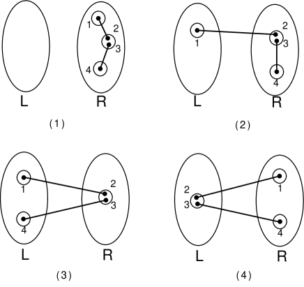
Figure 1: four different types of $2$-paths

The switching operations we are going to use are ideologically similar to the switching operations used by McKay and Wormald [10]. Although those switchings cannot be applied here because they do not preserve the property of the pairings being restricted, they can easily be adjusted and adapted to our current needs. The main twist is that there are a number of alternative switchings available use, and we need to specify which ones should be used, and for what values of the parameters, to achieve the desired result. The following two switching operations are used to prove Lemma 3.9.

(a) $L_{1}$-switching: take a loop $\{2,3\}$ and two pure pairs $\{1,5\},\ \{4,6\}$ such that the six points are located in the five distinct vertices as drawn in Figure 2. Replace the three pairs $\{2,3\},\{1,5\},\{4,6\}$ by $\{1,2\},\{3,4\},\{5,6\}$.

(b) $L_{2}$-switching: take a loop $\{2,3\}$ and two mixed pairs $\{1,5\},\ \{4,6\}$ such that the six points are located in the five distinct vertices as drawn in Figure 3. Replace the three pairs $\{2,3\},\{1,5\},\{4,6\}$ by $\{1,2\},\{3,4\},\{5,6\}$.

Figure 2: $L_{1}$-switching

Figure 3: $L_{2}$-switching

For any switching operation that converts a pairing $\mathcal{P}_{1}$ to another pairing $\mathcal{P}_{2}$, we call the operation that converts $\mathcal{P}_{2}$ to $\mathcal{P}_{1}$ the inverse of that switching. Thus, the inverse $L_{1}$-switching can be defined as follows. Take a 2-directed path (not necessarily simple) $((1,2),(3,4))$ of type 1 and a pure pair $\{5,6\}$ such that the points $1$, $2$, $4$, $5$ and $6$ lie in five distinct vertices. Replace $\{1,2\}$, $\{3,4\}$ and $\{5,6\}$ by $\{2,3\}$, $\{1,5\}$ and $\{4,6\}$. The inverse $L_{2}$-switching can be defined in the same way.

The following lemma estimates the ratio $|{\mathcal{C}}_{l_{0},l_{1},l_{2}}|/|{\mathcal{C}}_{l_{0}-1,l_{1},l_{2}}|$ by counting ways to perform certain $L_{1}$-switchings and their inverses. We express the present results in terms of the numbers $a_{i}(l_{0},l_{1},l_{2})$, defined in (3.7), whose estimation we postpone till later.

Lemma 3.9

Let $a_{1}=a_{1}(l_{0}-1,l_{1},l_{2})$ and $a_{3}=a_{3}(l_{0}-1,l_{1},l_{2})$. Assume $l_{0}\geq 1$. Then

$$(i): \mbox{If}\ t\geq 1,$$

$$\frac{|{\mathcal{C}}_{l_{0},l_{1},l_{2}}|}{|{\mathcal{C}}_{l_{0}-1,l_{1},l_{2}}|}=\frac{a_{1}}{4l_{0}t}(1+O(d_{\max}^{2}/t+(l_{0}+l_{2})/t)),$$

$$(ii): \mbox{If}\ M_{1}(L)\geq 1\ \mbox{and}\ t\geq 1,$$

$$\frac{|{\mathcal{C}}_{l_{0},l_{1},l_{2}}|}{|{\mathcal{C}}_{l_{0}-1,l_{1},l_{2}}|}=\frac{ta_{3}}{l_{0}M_{1}(L)^{2}}(1+O(d_{\max}^{2}/M_{1}(L)+d_{\max}^{2}/t+l_{1}/M_{1}(L)+(l_{0}+l_{2})/t)).$$

Proof.  Let $\mathcal{P}\in{\mathcal{C}}_{l_{0},l_{1},l_{2}}$ and we consider the number of $L_{1}$-switching operations that convert $\mathcal{P}$ to some $\mathcal{P}^{\prime}\in{\mathcal{C}}_{l_{0}-1,l_{1},l_{2}}$. For the purpose of counting, we label the points in the pairs that are under consideration as shown in Figure 2. So for any pair under consideration, we will incorporate in our counting the number of ways we can label the points in the pair. Let $N$ denote the number of ways to choose the pairs and label the points in them so that an $L_{1}$-switching can be applied to these pairs, which converts $\mathcal{P}$ to some $\mathcal{P}^{\prime}\in{\mathcal{C}}_{l_{0}-1,l_{1},l_{2}}$ without any simultaneously created loops or double pairs. This implies that the switching operations counted by $N$ destroy only one loop and there is no simultaneous creation or destruction of other loops or double pairs.

We first give a rough count of $N$, that includes some forbidden cases (due to creating double pairs, etc) and then estimate the error. There are $l_{0}$ ways to choose a loop $e_{0}$ and $t(t-1)$ ways to choose $(e_{1},e_{2})$, an ordered pair of two distinct pure pairs. For any chosen loop $e_{0}$, there are two ways to distinguish the two end points to label the points $2$ and $3$ as shown in Figure 2. For each of the other pairs, there are two ways to label its two endpoints, as $1$ and $5$, or $4$ and $6$, as the case may be. Hence a rough estimation of $N$ is $8l_{0}t(t-1)$, including the count of some forbidden choices of $e_{0}$, $e_{1}$ and $e_{2}$, which we estimate next. Let the vertices that contain points $2,1,5,6,4$ be denoted by $v_{0},v_{1},v_{2},v_{3},v_{4}$ respectively as shown in Figure 2. The only possible exclusions caused by invalid choices in the above are the following:

(a) the loop $e_{0}$ is adjacent to $e_{1}$ or $e_{2}$, or $e_{1}$ is adjacent to $e_{2}$, in which case, the $L_{1}$-switching is not applicable since the definition of the $L_{1}$-switching excludes cases where the edges are adjacent because it requires the end vertices to be distinct;

(b) there exists a pair between $\{v_{0},v_{1}\}$, or $\{v_{0},v_{4}\}$, or $\{v_{2},v_{3}\}$ in $\mathcal{P}$, in which case there will be more double pairs created after the $L_{1}$-switching is applied;

(c) the pair $e_{1}$ or $e_{2}$ is a loop or is contained in a double pair, in which case there is a simultaneously destroyed loop or double pair.

First we show that the number of exclusions from case (a) is $O(l_{0}td_{\max})$. The number of pairs of $(e_{0},e_{1})$ is at most $l_{0}t$. For any given $e_{0}$ and $e_{1}$, the number of ways to choose a pair $e_{2}$ such that $e_{2}$ is adjacent to $e_{0}$ or $e_{1}$ is at most $2d_{\max}$ since both $e_{0}$ and $e_{2}$ are adjacent to at most $d_{\max}$ pairs. Hence the number of triples of $(e_{0},e_{1},e_{2})$ such that $e_{2}$ is adjacent to either $e_{0}$ or $e_{1}$ is at most $2l_{0}td_{\max}$. By symmetry, the number of triples of $(e_{0},e_{1},e_{2})$ such that $e_{1}$ is adjacent to either $e_{0}$ or $e_{2}$ is also at most $2l_{0}td_{\max}$. Hence the number of exclusions from case (a) is $O(l_{0}td_{\max})$.

Next we show that the number of exclusions from case (b) is $O(l_{0}td_{\max}^{2})$. As just explained, the number of pairs of $(e_{0},e_{1})$ is at most $l_{0}t$. For any given $e_{0}$ and $e_{1}$, the number of ways to choose a pair $e_{2}$ such that $v_{3}$ is adjacent to $v_{2}$ or $v_{4}$ is adjacent to $v_{0}$ is at most $2d_{\max}^{2}$, since both $e_{0}$ and $e_{1}$ have at most $d_{\max}^{2}$ edges that are of distance $2$ away. Hence the number of triples $(e_{0},e_{1},e_{2})$ such that $v_{3}$ is adjacent to $v_{2}$ or $v_{4}$ is adjacent to $v_{0}$ is $O(l_{0}td_{\max}^{2})$. By symmetry, the number of triples $(e_{0},e_{1},e_{2})$ such that $v_{3}$ is adjacent to $v_{2}$ or $v_{0}$ is adjacent to $v_{1}$ is $O(l_{0}td_{\max}^{2})$. Hence the number of exclusions from case (b) is $O(l_{0}td_{\max}^{2})$.

Now we show that the number of exclusions from case (c) is $O(l_{0}^{2}t+l_{0}tl_{2})$. The number of ways to choose $e_{0},e_{1},e_{2}$ such that $e_{1}$ or $e_{2}$ is a loop is at most $2l_{0}^{2}t$ and the number of ways to choose these three pairs such that $e_{1}$ or $e_{2}$ is contained in a double pair is at most $2\cdot l_{0}t\cdot 2l_{2}=O(l_{0}tl_{2})$. Hence the number of exclusions from case (c) is $O(l_{0}^{2}t+l_{0}tl_{2})$.

Thus, the number of exclusions in the calculation of $N$ is $O(l_{0}td_{\max}^{2}+l_{0}^{2}t+l_{0}tl_{2})$. So $N=8l_{0}t^{2}(1+O(d_{\max}^{2}/t+(l_{0}+l_{2})/t))$.

Now choose an arbitrary pairing $\mathcal{P}^{\prime}\in{\mathcal{C}}_{l_{0}-1,l_{1},l_{2}}$. Let $N^{\prime}$ be the number of ways to choose the pairs and label points in them so that an inverse $L_{1}$-switching operation can be applied to these pairs such that $\mathcal{P}^{\prime}$ is converted to some $\mathcal{P}\in{\mathcal{C}}_{l_{0},t_{1},t_{2}}$ without any simultaneously destroyed loops or double pairs. To apply this operation we need to choose $e^{\prime}_{0},e^{\prime}_{1},e^{\prime}_{2}$, such that $(e^{\prime}_{0},e^{\prime}_{1})$ is a simple directed 2-path of type 1 and $e^{\prime}_{2}$ is a pure pair. We consider the directed 2-path $(e^{\prime}_{0},e^{\prime}_{1})$ because it automatically gives a unique way of distinguishing vertices $v_{1}$, $v_{0}$ and $v_{4}$ and labelling points as $1$, $2$, $3$ and $4$ in Figure 2. There are $A_{1}(\mathcal{P}^{\prime})$ simple directed $2$-paths of type 1, and hence $A_{1}(\mathcal{P}^{\prime})$ ways to choose the points as $1$, $2$, $3$ and $4$. The number of ways to choose a pure pair $e^{\prime}_{2}$ is $t$ and so there are $2t$ ways to fix the vertices $v_{2}$, $v_{3}$ and the points $\{5,6\}$. The only possible exclusions to the above choices are listed the following cases.

(a) There exists a pair between $\{v_{1},v_{2}\}$ or $\{v_{3},v_{4}\}$ in $\mathcal{P}^{\prime}$, since then more double pairs will be created if the inverse $L_{1}$-switching is applied.

(b) The pair $e^{\prime}_{2}$ is a loop, in which case the inverse $L_{1}$-switching is not applicable, or $e^{\prime}_{2}$ is contained in a double pair, in which case a double pair is destroyed after the application of the inverse $L_{1}$-switching.

(c) The pair $e_{2}^{\prime}$ is adjacent to the 2-path or is contained in the 2-path, in which case the inverse $L_{1}$-switching operation is not applicable.

The number of exclusions from case (a) is $O(A_{1}(\mathcal{P}^{\prime})d_{\max}^{2})$ and the numbers of exclusions from case (b) and (c) are $O(A_{1}(\mathcal{P}^{\prime})l_{0}+A_{1}(\mathcal{P}^{\prime})l_{2})$ and $O(A_{1}(\mathcal{P}^{\prime})d_{\max})$ respectively.

Thus, the number of exclusions from case (a)–(d) is $O(A_{1}(\mathcal{P}^{\prime})d_{\max}^{2}+A_{1}(\mathcal{P}^{\prime})l_{0}+A_{1}(\mathcal{P}^{\prime})l_{2})$. So

$${\bf E}(N^{\prime})={\bf E}\big{(}2A_{1}t(1+O(d_{\max}^{2}/t+(l_{0}+l_{2})/t))\mid\mathcal{P}^{\prime}\in{\mathcal{C}}_{l_{0}-1,l_{1},l_{2}}\big{)}=2a_{1}t(1+O(d_{\max}^{2}/t+(l_{0}+l_{2})/t)).$$

We count the pairs of $(\mathcal{P},\mathcal{P}^{\prime})$ such that $\mathcal{P}\in{\mathcal{C}}_{l_{0},t_{1},t_{2}}$, $\mathcal{P}^{\prime}\in{\mathcal{C}}_{l_{0}-1,l_{1},l_{2}}$, and $\mathcal{P}^{\prime}$ is obtained by applying an $L_{1}$-switching to $\mathcal{P}$, which destroys only one loop without any simultaneously created loops or double pairs. Then the number of such pairs of pairings equals to both $|{\mathcal{C}}_{l_{0},l_{1},l_{2}}|{\bf E}(N)$ and $|{\mathcal{C}}_{l_{0}-1,l_{1},l_{2}}|{\bf E}(N^{\prime})$. Thus,

$$\frac{|{\mathcal{C}}_{l_{0},l_{1},l_{2}}|}{|{\mathcal{C}}_{l_{0}-1,l_{1},l_{2}}|}=\frac{a_{1}}{4l_{0}t}(1+O(d_{\max}^{2}/t+(l_{0}+l_{2})/t)).$$

This proves part (i) of Lemma 3.9. Analogously we can deduce the following by analysing the $L_{2}$-switching and its inverse.

$$\frac{|{\mathcal{C}}_{l_{0},l_{1},l_{2}}|}{|{\mathcal{C}}_{l_{0}-1,l_{1},l_{2}}|} = \frac{2ta_{3}+O(d_{\max}^{2}a_{3})+O(l_{0}a_{3}+l_{2}a_{3})}{2l_{0}M_{1}(L)^{2}+O(d_{\max}^{2}M_{1}(L)l_{0}+l_{0}M_{1}(L)l_{1})}$$

$$= \frac{ta_{3}}{l_{0}M_{1}(L)^{2}}(1+O(d_{\max}^{2}/M_{1}(L)+d_{\max}^{2}/t+(l_{0}+l_{2})/t+l_{1}/M_{1}(L))).$$

Then we obtain part (ii) of Lemma 3.9.    

We use the following two switching operations to prove Lemma 3.10.

(a) $D_{1}$-switching: take a mixed double pair $\{\{3,4\},\{5,6\}\}$ and also two pure pairs $\{1,2\}$ and $\{7,8\}$ such that the eight points are located in the six distinct vertices as shown in Figure 4. Replace the four pairs by $\{1,3\},\{5,7\},\{2,4\},\{6,8\}$.

Figure 4: $D_{1}$-switching

(b) $D_{2}$-switching: take a mixed double pair $\{\{3,4\},\{5,6\}\}$ and also two mixed pairs $\{1,2\}$ and $\{7,8\}$ such that the eight points are located in the six distinct vertices as shown in Figure 5. Replace the four pairs by $\{1,4\},\{6,7\},\{2,3\},\{5,8\}$.

Figure 5: $D_{2}$-switching

The inverse switchings are defined analogously to the earlier ones. For instance, the inverse $D_{1}$-switching is defined as follows. Take a directed $2$-path $((1,3),(5,7))$ of type $4$ and a directed $2$-path $((2,4),(6,8))$ of type $1$ such that the eight points are located in six distinct vertices as shown in Figure 4. Replace these four pairs by $\{1,2\}$, $\{3,4\}$, $\{5,6\}$ and $\{7,8\}$.

Lemma 3.10

Let $a_{1}=a_{1}(0,l_{1}-1,l_{2})$ and $a_{3}=a_{3}(0,l_{1}-1,l_{2})$. Assume $l_{1}\geq 1$. Then

$$(i): \mbox{If}\ t\geq 1\ \mbox{and}\ M_{2}(L)\geq 1,$$

$$\frac{|{\mathcal{C}}_{0,l_{1},l_{2}}|}{|{\mathcal{C}}_{0,l_{1}-1,l_{2}}|}=\frac{M_{2}(L)a_{1}}{8l_{1}t^{2}}(1+O(d_{\max}^{3}/M_{2}(L)+d_{\max}^{2}/t+l_{2}/t+l_{1}d_{\max}/M_{2}(L)));$$

$$(ii): \mbox{If}\ M_{1}(L)\geq 1\ \mbox{and}\ M_{2}(L)\geq 1,$$

$$\frac{|{\mathcal{C}}_{0,l_{1},l_{2}}|}{|{\mathcal{C}}_{0,l_{1}-1,l_{2}}|}=\frac{a_{3}M_{2}(L)}{2l_{1}M_{1}(L)^{2}}(1+O(d_{\max}^{2}/M_{1}(L)+d_{\max}^{3}/M_{2}(L)+l_{1}/M_{1}(L)+l_{1}d_{\max}/M_{2}(L))).$$

Proof.  For a given pairing $\mathcal{P}\in{\mathcal{C}}_{0,l_{1},l_{2}}$, let $N$ be the number of ways to choose the pairs and label the points in them so that a $D_{1}$-switching can be applied to these pairs such that $\mathcal{P}$ is converted to some $\mathcal{P}^{\prime}\in{\mathcal{C}}_{0,l_{1}-1,l_{2}}$ without simultaneously creating any loops and double pairs. In order to apply a $D_{1}$-switching operation, we need to choose a mixed double pair $\{e_{1},e_{2}\}$ and an ordered pair of distinct pure pairs $(e_{3},e_{4})$. The number of ways to choose $\{e_{1},e_{2}\}$ is $l_{1}$ in ${\mathcal{C}}_{0,l_{1},l_{2}}$ and hence the number of ways to label the points as $3,4,5,6$ is $2l_{1}$. The number of ways to choose the ordered pair of pure pairs $(e_{3},e_{4})$ is $t(t-1)$. For any chosen $(e_{3},e_{4})$, there are 4 ways to label points as $1,2,7,8$. Let the vertices that contain points $3,4,1,2,7,8$ be $v_{1},v_{2},v_{3},v_{4},v_{5},v_{6}$ as shown in Figure 4. Hence a rough count of $N$ is $8l_{1}t(t-1)$ including the count of a few forbidden choices of $e_{1},e_{2},e_{3},e_{4}$, which are listed as follows.

(a) The pair $e_{1}$ is adjacent to $e_{3}$ or $e_{4}$, or $e_{3}$ is adjacent to $e_{4}$, in which case the $D_{1}$-switching is not applicable.

(b) There exists a pair between $\{v_{1},v_{3}\}$, or $\{v_{2},v_{4}\}$, or $\{v_{2},v_{6}\}$, or $\{v_{1},v_{5}\}$ in $\mathcal{P}$, since another double pair will be created after the $D_{1}$-switching is applied.

(c) The pair $e_{3}$ or $e_{4}$ is contained in a double pair, since another double pair is destroyed after the $D_{1}$-switching is applied.

The numbers of forbidden choices of $e_{1},e_{2},e_{3},e_{4}$ coming from case (a), (b) and (c) are $O(l_{1}td_{\max})$, $O(l_{1}td_{\max}^{2})$ and $O(l_{1}tl_{2})$ respectively. So $N=8l_{1}t^{2}(1+O(d_{\max}^{2}/t+l_{2}/t))$.

For a given pairing $\mathcal{P}^{\prime}\in{\mathcal{C}}_{0,l_{1}-1,l_{2}}$, let $N^{\prime}$ be the number of ways to choose the pairs and label the points in them so that an inverse $D_{1}$-switching operation can be applied to these pairs which converts $\mathcal{P}^{\prime}$ to some $\mathcal{P}\in{\mathcal{C}}_{0,l_{1},l_{2}}$ without destroying any loops or double pairs simultaneously. In order to apply such an operation, we need to choose two simple directed 2-paths, one of type 1 and the other of type 4. There are $A_{1}(\mathcal{P}^{\prime})$ simple directed 2-paths of type 1, each of which gives a way of labelling points as $2,4,6,8$, and there are $A_{4}(\mathcal{P}^{\prime})$ simple directed 2-paths of type 4, each of which gives a way of labelling points as $1,3,5,7$. Hence a rough count of $N^{\prime}$ is $A_{1}(\mathcal{P}^{\prime})A_{4}(\mathcal{P}^{\prime})$ including the counts of a few forbidden choices of such two 2-paths which are listed in the following two cases.

(a) If we have $v_{i}=v_{j}$, for $i\in\{3,5\}$ and $j\in\{2,4,6\}$, then the operation is not applicable.

(b) If there already exists a pair between $\{v_{1},v_{2}\}$, or $\{v_{3},v_{4}\}$, or $\{v_{5},v_{6}\}$ in $\mathcal{P}^{\prime}$, then more than one double pair will be created in this case if the inverse $D_{1}$-switching is applied.

The numbers of forbidden choices of the two directed 2-paths from case (a) and (b) are respectively $O(A_{1}(\mathcal{P}^{\prime})d_{\max}^{2})=O(a_{1}d_{\max}^{2})$ and $O(A_{1}(\mathcal{P}^{\prime})d_{\max}^{3})=O(a_{1}d_{\max}^{3})$. So ${\bf E}(N^{\prime})={\bf E}\big{(}A_{1}(\mathcal{P}^{\prime})A_{4}(\mathcal{P}^{\prime})\mid\mathcal{P}^{\prime}\in{\mathcal{C}}_{0,l_{1}-1,l_{2}}\big{)}+O(a_{1}d_{\max}^{3})=a_{1}(M_{2}(L)-O(l_{1}d_{\max}))(1+O(d_{\max}^{3}/M_{2}(L)))$. Since $l_{1}\geq 1$, we have $M_{2}(L)\geq 1$. Hence

$$\frac{|{\mathcal{C}}_{0,l_{1},l_{2}}|}{|{\mathcal{C}}_{0,l_{1}-1,l_{2}}|} = \frac{a_{1}M_{2}(L)(1+O(d_{\max}^{3}/M_{2}(L))+O(l_{1}d_{\max}/M_{2}(L)))}{8l_{1}t^{2}(1+O(d_{\max}^{2}/t)+O(l_{2}/t))}$$

$$= \frac{a_{1}M_{2}(L)}{8l_{1}t^{2}}(1+O(d_{\max}^{3}/M_{2}(L)+d_{\max}^{2}/t+l_{2}/t+l_{1}d_{\max}/M_{2}(L))),$$

and this shows part (i) of Lemma 3.10. Similarly we can obtain part (ii) by analysing the $D_{2}$-switching and its inverse.    

The following two switching operations are used for the next lemma.

(a) $D_{3}$-switching: take a pure double pair $\{\{1,2\},\{3,4\}\}$ and also two pure pairs $\{5,6\}$ and $\{7,8\}$ such that the eight points are located in the six distinct vertices as shown in Figure 6. Replace the four pairs by $\{1,5\},\{2,6\},\{3,7\},\{4,8\}$.

Figure 6: $D_{3}$-switching

(a) $D_{4}$-switching: take a pure double pair $\{\{1,2\},\{3,4\}\}$ and also four mixed pairs $\{5,6\}$, $\{7,8\}$, $\{9,10\}$, $\{11,12\}$ such that the twelve points are located in the ten distinct vertices as shown in Figure 7. Replace the six pairs by $\{6,10\},\{8,12\},\{1,5\},\{3,9\}$,$\{2,11\}$, $\{4,7\}$.

Figure 7: $D_{4}$-switching

The inverse switchings are defined in the obvious way. For example, for the inverse of the $D_{3}$-switching, take two directed paths of type 1, $((5,1),(3,7))$ and $((6,2),(4,8))$, such that the eight points are located in six distinct vertices as shown in Figure 6. Replace these four pairs by $\{5,6\}$, $\{1,2\}$, $\{3,4\}$, $\{7,8\}$. Define $b_{i}(l_{0},l_{1},l_{2})={\bf E}(A_{i}(\mathcal{P})^{2}\mid\mathcal{P}\in{\mathcal{C}}_{l_{0},l_{1},l_{2}})$ for $i=1$ and $3$.

Lemma 3.11

Assume $l_{2}\geq 1$. For $i=1,3$, let $b_{i}=b_{i}(0,0,l_{2}-1)$ for short. Then

$$(i): \mbox{If}\ t\geq 1\ \mbox{and}\ b_{1}\geq 1,$$

$$\frac{|{\mathcal{C}}_{0,0,l_{2}}|}{|{\mathcal{C}}_{0,0,l_{2}-1}|}=\frac{b_{1}}{16l_{2}t^{2}}(1+O(d_{\max}^{2}/t+d_{\max}^{3}a_{1}/b_{1}+l_{2}/t)).$$

$$(ii): \mbox{If}\ M_{1}(L)\geq 1,\ b_{3}\geq 1\ \mbox{and}\ t\geq 1,$$

$$\frac{|{\mathcal{C}}_{0,0,l_{2}}|}{|{\mathcal{C}}_{0,0,l_{2}-1}|}=\frac{t^{2}b_{3}}{l_{2}M_{1}(L)^{4}}(1+O(d_{\max}^{3}a_{3}/b_{3}+d_{\max}^{2}/M_{1}(L)+l_{2}/t)).$$

Proof.  For a given pairing $\mathcal{P}\in{\mathcal{C}}_{0,0,l_{2}}$, let $N$ be the number of ways to choose the pairs and label the points in them so that a $D_{3}$-switching operation can be applied, which converts $\mathcal{P}$ to some $\mathcal{P}^{\prime}\in{\mathcal{C}}_{0,0,l_{2}-1}$ without creating any loops and double pairs simultaneously. In order to apply a $D_{3}$-switching operation, we need to choose a pure double pair $\{e_{1},e_{2}\}$ and an ordered pair of distinct pure pairs $(e_{3},e_{4})$. The number of ways to choose $\{e_{1},e_{2}\}$ is $l_{2}$ in ${\mathcal{C}}_{0,0,l_{2}}$ and there are four ways to label the points as $1,2,3,4$ for any chosen double pair. The number of ways to choose an ordered pair of two pure pairs $(e_{3},e_{4})$ is $t(t-1)$ and hence the number of ways to label the points as $5,6,7,8$ is $4t(t-1)$. Hence a rough count of $N$ is $16l_{2}t(t-1)$ including the counts of forbidden choices of pairs $e_{1},\ldots,e_{4}$ which we estimate next. Let the vertices that contain points $1,2,5,6,7,8$ be $v_{1},v_{2},v_{3},v_{4},v_{5},v_{6}$ as shown in Figure 6. The forbidden choices of the pairs $e_{1},\ldots,e_{4}$ are listed in the following three cases.

(a) When $e_{1}$ is adjacent to $e_{3}$ or $e_{4}$ or when $e_{3}$ is adjacent to $e_{4}$, then the $D_{3}$-switching is not applicable.

(b) If there exists a pair between $\{v_{1},v_{3}\}$, or $\{v_{2},v_{4}\}$, or $\{v_{1},v_{5}\}$, or $\{v_{2},v_{6}\}$ in $\mathcal{P}$, then more double pairs will be created after the application of the switching operation.

(c) If $e_{3}$ or $e_{4}$ is contained in a double pair, then another double pair would be destroyed after the application of the switching operation.

The numbers of forbidden choices of $e_{1},\ldots,e_{4}$ coming from (a),(b) and (c) are $O(l_{2}td_{\max})$, $O(l_{2}td_{\max}^{2})$ and $O(l_{2}^{2}t)$ respectively. So $N=16l_{2}t^{2}(1+O(d_{\max}^{2}/t+l_{2}/t))$.

For any pairing $\mathcal{P}^{\prime}\in{\mathcal{C}}_{0,0,l_{2}-1}$, let $N^{\prime}$ be the number of ways to choose the pairs and label the points in them so that an inverse $D_{3}$-switching can be applied to these pairs, which converts $\mathcal{P}^{\prime}$ to some $\mathcal{P}\in{\mathcal{C}}_{0,0,l_{2}}$ without simultaneously destroying any loops or double pairs. In order to apply such an operation, we need to choose an ordered pair of distinct simple directed 2-paths of type 1. The number of ways to do that is $A_{1}(\mathcal{P}^{\prime})(A_{1}(\mathcal{P}^{\prime})-1)$. So the number of ways to label the points $1,2,\ldots,8$ is $A_{1}(\mathcal{P}^{\prime})(A_{1}(\mathcal{P}^{\prime})-1)$, which gives a rough count of $N^{\prime}$. The forbidden choices of the two paths whose counts should be excluded from $N^{\prime}$ are listed in the following cases.

(a) The two paths share some common vertex or common pair. In this case the inverse $D_{3}$-switching is not applicable.

(b) There exists a pair between $\{v_{1},v_{2}\}$ or $\{v_{3},v_{4}\}$ or $\{v_{5},v_{6}\}$ in $\mathcal{P}^{\prime}$. In this case, more double pairs will be created after the inverse $D_{3}$-switching operation is applied.

The numbers of ways to choose the ordered pair of 2-paths in case (a) and (b) are $O(A_{1}(\mathcal{P}^{\prime})d_{\max}^{2})$ and $O(A_{1}(\mathcal{P}^{\prime})d_{\max}^{3})$ respectively. Thus, ${\bf E}(N^{\prime})=b_{1}(1+O(d_{\max}^{3}a_{1}/b_{1}))$.

Hence

$$\frac{|{\mathcal{C}}_{0,0,l_{2}}|}{|{\mathcal{C}}_{0,0,l_{2}-1}|}=\frac{b_{1}}{16l_{2}t^{2}}(1+O(d_{\max}^{2}/t+d_{\max}^{3}a_{1}/b_{1}+(l_{0}+l_{2})/t)).$$

Similarly by analysing the $D_{4}$-switching and its inverse, we obtain Lemma 3.11(ii).   

4 More switchings to estimate $a$’s and $b$’s

The lemmas in the previous section give ratios of the sizes of ‘adjacent’ classes ${\mathcal{C}}_{i,j,k}$, but those estimates are in terms of $a_{i}(l_{0},l_{1},l_{2})$ ($i=1,2,3$) defined in (3.7), $b_{i}$ ($i=1,3$) defined just before Lemma 3.11, and $t$ defined in (3.6). In this section, we use further switchings to estimate the values of these variables. The following two switchings are used for $a_{i}$.

(a) $S_{1}$-switching: Take a mixed pair and label the points in it by $\{1,2\}$ as shown in Figure 8. Take a simple directed $2$-path that is vertex disjoint from the chosen mixed pair. Label the points by $3,4,5,6$. Replace these three pairs by $\{2,3\}$, $\{1,4\}$ and $\{5,6\}$.

Figure 8: $S_{1}$-switching

(b) $S_{2}$ switching: Take a pure pair $\{5,6\}$ and a simple directed $2$-path $((1,2),(3,4))$ such that the six points are located in five distinct vertices shown as in Figure 9. Replace these three pairs by $\{1,2\}$, $\{3,5\}$ and $\{4,6\}$.

Figure 9: $S_{2}$-switching

The inverse switchings are defined in the obvious way.

Lemma 4.1

Given $l_{0}$, $l_{1}$ and $l_{2}$, let $\ell=l_{0}+l_{1}+l_{2}$. We have

$$(i): \mbox{if}\ M_{1}(L)\leq M/4\ \mbox{and}\ M_{2}(R)\geq 1,$$

$$a_{1}(l_{0},l_{1},l_{2})=\frac{(M_{1}(R)-M_{1}(L))^{2}M_{2}(R)}{M_{1}(R)^{2}}(1+O(d_{\max}^{2}/t+\ell/t+(\ell d_{\max}+l_{0}d_{\max}^{2})/M_{2}(R)));$$

$$(ii): \mbox{if}\ M_{1}(L)>M/4\ \mbox{and}\ M_{2}(R)\geq 1,$$

$$a_{3}(l_{0},l_{1},l_{2})=\frac{M_{1}(L)^{2}M_{2}(R)}{M_{1}(R)^{2}}(1+O(d_{\max}^{2}/M_{1}(L)+\ell/M_{1}(L)+(\ell d_{\max}+l_{0}d_{\max}^{2})/M_{2}(R))).$$

Proof.  Let $a_{i}=a_{i}(l_{0},l_{1},l_{2})$ for $i=1,2,3$. We use the $S_{1}$-switching to compute the ratio $a_{1}/a_{2}$ and the $S_{2}$-switching to compute the ratio $a_{3}/a_{2}$. We count the ordered pairs of pairings $(\mathcal{P},\mathcal{P}^{\prime})$ such that both $\mathcal{P}$ and $\mathcal{P}^{\prime}$ are from ${\mathcal{C}}_{l_{0},l_{1},l_{2}}$, and $\mathcal{P}^{\prime}$ is obtained from $\mathcal{P}$ by applying an $S_{1}$-switching to $\mathcal{P}$ without any creation or destruction of loops or double pairs. Let $N_{1}$ denote the number of such ordered pairs of pairings.

We first prove part (i). Assume $M_{1}(L)\leq M/4$. For any directed 2-path of type 1 in ${\mathcal{C}}_{l_{0},l_{1},l_{2}}$, the number of $S_{1}$-switching operations that can be applied to it is

$$A_{1}M_{1}(L)+O(A_{1}d_{\max}^{2}+A_{1}l_{1})=A_{1}M_{1}(L)\Big{(}1+O(d_{\max}^{2}/M_{1}(L)+l_{1}/M_{1}(L))\Big{)}.$$ (4.1)

For any directed 2-path of type 2 in ${\mathcal{C}}_{l_{0},l_{1},l_{2}}$, the number of inverse $S_{1}$-switching operations that can be applied to it is

$$A_{2}\cdot 2t+O(A_{2}d_{\max}^{2}+A_{2}(l_{0}+l_{2}))=A_{2}\cdot 2t\Big{(}1+O(d_{\max}^{2}/t+(l_{0}+l_{2})/t)\Big{)}.$$ (4.2)

The total number of $S_{1}$-switching operations that can be applied to pairings in ${\mathcal{C}}_{l_{0},l_{1},l_{2}}$ is

$$\sum_{\mathcal{P}\in{\mathcal{C}}_{l_{0},l_{1},l_{2}}}A_{1}(\mathcal{P})M_{1}(L)\Big{(}1+O((d_{\max}^{2}+l_{1})/M_{1}(L))\Big{)}=a_{1}M_{1}(L)\Big{(}1+O((d_{\max}^{2}+\ell)/M_{1}(L))\Big{)}|{\mathcal{C}}_{l_{0},l_{1},l_{2}}|,$$

and the total number of inverse $S_{1}$-switching operations that can be applied to pairings in ${\mathcal{C}}_{l_{0},l_{1},l_{2}}$ is

$$\sum_{\mathcal{P}\in{\mathcal{C}}_{l_{0},l_{1},l_{2}}}A_{2}(\mathcal{P})\cdot 2t\Big{(}1+O(d_{\max}^{2}/t+(l_{0}+l_{2})/t)\Big{)}=a_{2}\cdot 2t\Big{(}1+O(d_{\max}^{2}/t+\ell/t)\Big{)}|{\mathcal{C}}_{l_{0},l_{1},l_{2}}|.$$

These two numbers are both equal to $N_{1}$. Hence

$$\frac{a_{2}}{a_{1}} = \frac{M_{1}(L)}{2t}(1+O(d_{\max}^{2}/t+d_{\max}^{2}/M_{1}(L)+\ell/M_{1}(L)+\ell/t)).$$ (4.3)

Similarly, by the $S_{2}$-switching and its inverse we get

$$\frac{a_{3}}{a_{2}} = \frac{M_{1}(L)}{2t}(1+O(d_{\max}^{2}/t+d_{\max}^{2}/M_{1}(L)+\ell/M_{1}(L)+\ell/t)).$$ (4.4)

Then (4.3) gives

$$\frac{a_{2}}{a_{1}}=\frac{M_{1}(L)}{2t}\Big{(}1+O((d_{\max}^{2}+\ell)/t)\Big{)}+O((d_{\max}^{2}+\ell)/t),$$

and (4.4) gives

$$\frac{a_{3}}{a_{2}}=\frac{M_{1}(L)}{2t}\Big{(}1+O((d_{\max}^{2}+\ell)/t)\Big{)}+O((d_{\max}^{2}+\ell)/t).$$

Hence

$$a_{2} = a_{1}\left(\frac{M_{1}(L)}{2t}\Big{(}1+O((d_{\max}^{2}+\ell)/t)\Big{)}+O((d_{\max}^{2}+\ell)/t)\right)$$

$$a_{3} = a_{1}\left(\frac{M_{1}(L)}{2t}\Big{(}1+O((d_{\max}^{2}+\ell)/t)\Big{)}+O((d_{\max}^{2}+\ell)/t)\right)^{2}.$$

Since $M_{1}(L)\leq M/4$, we have $M_{1}(L)/t\leq 1$ and so

$$a_{3}=a_{1}\left(\left(\frac{M_{1}(L)}{2t}\right)^{2}\Big{(}1+O((d_{\max}^{2}+\ell)/t)\Big{)}+O((d_{\max}^{2}+\ell)/t)\right).$$

Hence

$$a_{1}+2a_{2}+a_{3} = a_{1}\left(1+\left(2\frac{M_{1}(L)}{2t}+\left(\frac{M_{1}(L)}{2t}\right)^{2}\right)\Big{(}1+O((d_{\max}^{2}+\ell)/t)\Big{)}+O((d_{\max}^{2}+\ell)/t)\right)$$ (4.5)

$$= a_{1}\left(\left(1+\frac{M_{1}(L)}{2t}\right)^{2}\Big{(}1+O((d_{\max}^{2}+\ell)/t)\Big{)}+O((d_{\max}^{2}+\ell)/t)\right)$$

$$= a_{1}\left(1+\frac{M_{1}(L)}{2t}\right)^{2}(1+O((d_{\max}^{2}+\ell)/t)).$$

For any pairing $\mathcal{P}\in{\mathcal{C}}_{l_{0},l_{1},l_{2}}$, the number of simple directed $2$-paths in $\mathcal{P}$ is $\sum_{v\in L\cup R}d(v)(d(v)-1)-O(\ell d_{\max}+l_{0}d_{\max}^{2})$, since the number of non-simple directed 2-path is bounded by $O(l_{0}d_{\max}^{2}+l_{1}d_{\max}+l_{2}d_{\max})=O(\ell d_{\max}+l_{0}d_{\max}^{2})$. On the other hand, the number of simple directed $2$-paths in $\mathcal{P}$ is $A_{1}+2A_{2}+A_{3}+A_{4}$, since $2A_{2}$ counts the number of directed 2-paths of type 2 and the opposite direction. Then

$$A_{1}+2A_{2}+A_{3}+M_{2}(L)-O(l_{1}d_{\max})=\sum_{v\in L\cup R}d(v)(d(v)-1)-O(\ell d_{\max}+l_{0}d_{\max}^{2}).$$

Thus,

$$A_{1}+2A_{2}+A_{3}=M_{2}(R)+O(\ell d_{\max}+l_{0}d_{\max}^{2})=M_{2}(R)(1+O((\ell d_{\max}+l_{0}d_{\max}^{2})/M_{2}(R))).$$ (4.6)

Combining this with (4.5), we have

$$a_{1}=\frac{(M_{1}(R)-M_{1}(L))^{2}M_{2}(R)}{M_{1}(R)^{2}}(1+O(d_{\max}^{2}/t+\ell/t+(\ell d_{\max}+l_{0}d_{\max}^{2})/M_{2}(R))),$$

which proves part (i).

Next we show part (ii). Assume $M_{1}(L)>M/4$. We observe that (4.3) also gives

$$\frac{a_{1}}{a_{2}}=\frac{2t}{M_{1}(L)}\Big{(}1+O((d_{\max}^{2}+\ell)/M_{1}(L))\Big{)}+O((d_{\max}^{2}+\ell)/M_{1}(L)),$$

and (4.4) gives

$$\frac{a_{2}}{a_{3}}=\frac{2t}{M_{1}(L)}\Big{(}1+O((d_{\max}^{2}+\ell)/M_{1}(L))\Big{)}+O((d_{\max}^{2}+\ell)/M_{1}(L)).$$

Thus,

$$a_{2} = a_{3}\left(\frac{2t}{M_{1}(L)}\Big{(}1+O((d_{\max}^{2}+\ell)/M_{1}(L))\Big{)}+O((d_{\max}^{2}+\ell)/M_{1}(L))\right)$$

$$a_{1} = a_{3}\left(\frac{2t}{M_{1}(L)}\Big{(}1+O((d_{\max}^{2}+\ell)/M_{1}(L))\Big{)}+O((d_{\max}^{2}+\ell)/M_{1}(L))\right).$$

Since $M_{1}(L)\geq 1/4$, we have $t/M_{1}(L)<1$ and so

$$a_{1}+2a_{2}+a_{3} = a_{3}\left(1+\frac{2t}{M_{1}(L)}\right)^{2}\Big{(}1+O((d_{\max}^{2}+\ell)/M_{1}(L))\Big{)}$$

$$= M_{2}(R)(1+O((\ell d_{\max}+l_{0}d_{\max}^{2})/M_{2}(R))).$$

Hence

$$a_{3}=\frac{M_{1}(L)^{2}M_{2}(R)}{M_{1}(R)^{2}}(1+O(d_{\max}^{2}/M_{1}(L)+\ell/M_{1}(L)+(\ell d_{\max}+l_{0}d_{\max}^{2})/M_{2}(R))).$$

This proves part (ii) of the lemma.    

Recall the definition of $b_{i}(l_{0},l_{1},l_{2})$ above Lemma 3.11. We next estimate these using simple modifications of the $S_{i}$-switchings for $i=1,3$. (Note: in this lemma, our abbreviation $b_{i}$ contains no shift of index, whilst it did in Lemma 3.11.)

Lemma 4.2

For $i=1,3$, let $a_{i}=a_{i}(l_{0},l_{1},l_{2})$ and $b_{i}=b_{i}(l_{0},l_{1},l_{2})$, and let $\ell=l_{0}+l_{1}+l_{2}$. Assume $M_{2}(R)\geq 1$. Then

$$(i): \mbox{if}\ M_{1}(L)\leq M/4,\ \ b_{1}=a_{1}^{2}(1+O(d_{\max}^{2}/t+\ell/t+(\ell d_{\max}+l_{0}d_{\max}^{2}+d_{\max}^{3})/M_{2}(R)));$$

$$(ii): \mbox{if}\ M_{1}(L)>M/4,$$

$$b_{3}=a_{3}^{2}(1+O(d_{\max}^{2}/M_{1}(L)+\ell/M_{1}(L)+(\ell d_{\max}+l_{0}d_{\max}^{2}+d_{\max}^{3})/M_{2}(R))).$$

Proof.  For $1\leq i\leq 5$, let $X_{i}(\mathcal{P})$ denote the number of ordered pairs of vertex disjoint simple $2$-paths in $\mathcal{P}$ where the first path has type $j_{i}$ and the second has type $h_{i}$, with $(j_{1},h_{1})=(1,1)$, $(j_{2},h_{2})=(3,3)$, $(j_{3},h_{3})=(1,2)$, $(j_{4},h_{4})=(1,3)$, and $(j_{3},h_{3})=(2,3)$.

The $S_{3}$-switching, as illustrated in Figure 10, is a slight modification of the $S_{1}$-switching. To apply it, we need to choose a mixed pair and two simple $2$-paths of type 1 such that they are pairwise disjoint. To apply its inverse, we need to choose a pure pair and two simple $2$-paths of type 2 and 1 respectively such that they are pairwise disjoint. Compared with the $S_{1}$-switching, the $S_{3}$-switching requires an additional simple directed $2$-path of type $1$. However, the pairs in the extra $2$-path remain after the $S_{3}$-switching is applied since the mixed pair and the other simple directed $2$-path under consideration are vertex-disjoint from the additional directed $2$-path. The $S_{4}$-switching, as illustrated in Figure 11, is a similar modification of the $S_{2}$-switching.

We will first estimate ${\bf E}(X_{i}(\mathcal{P})\mid\mathcal{P}\in{\mathcal{C}}_{l_{0},l_{1},l_{2}})$ for $i\in[5]$ and then use this to estimate $b_{1}$ and $b_{3}$. Following the analogous argument as in Lemma 4.1, we can estimate the ratio ${\bf E}(X_{3}(\mathcal{P})\mid\mathcal{P}\in{\mathcal{C}}_{l_{0},l_{1},l_{2}})/{\bf E}(X_{1}(\mathcal{P})\mid\mathcal{P}\in{\mathcal{C}}_{l_{0},l_{1},l_{2}})$ by counting the ordered pairs of pairings $(\mathcal{P},\mathcal{P}^{\prime})$ such that $\mathcal{P},\mathcal{P}^{\prime}\in{\mathcal{C}}_{l_{0},l_{1},l_{2}}$ and $\mathcal{P}^{\prime}$ is obtained by applying an $S_{3}$-operation to $\mathcal{P}$ without any creation or destruction of loops or double pairs. The the number of such $S_{3}$-switching operations that can be applied to $\mathcal{P}$ is $X_{1}M_{1}(L)+O(X_{1}d_{\max}^{2}+X_{1}l_{1})$. The number of such inverse $S_{3}$-operations that can be applied to $\mathcal{P}$ is $2tX_{3}+O(X_{3}d_{\max}^{2}+X_{3}(l_{0}+l_{2}))$. So the ratio ${\bf E}(X_{3}(\mathcal{P})\mid\mathcal{P}\in{\mathcal{C}}_{l_{0},l_{1},l_{2}})/{\bf E}(X_{1}(\mathcal{P})\mid\mathcal{P}\in{\mathcal{C}}_{l_{0},l_{1},l_{2}})$ equals exactly the right hand side of (4.3) and the ratio ${\bf E}(X_{4}(\mathcal{P})\mid\mathcal{P}\in{\mathcal{C}}_{l_{0},l_{1},l_{2}})/{\bf E}(X_{3}(\mathcal{P})\mid\mathcal{P}\in{\mathcal{C}}_{l_{0},l_{1},l_{2}})$ equals exactly the right hand side of (4.4).

Figure 10: $S_{3}$-switching

Figure 11: $S_{4}$-switching

On the other hand, by (4.6), for any $\mathcal{P}\in{\mathcal{C}}_{l_{0},l_{1},l_{2}}$, $A_{1}(\mathcal{P})+2A_{2}(\mathcal{P})+A_{3}(\mathcal{P})=M_{2}(R)(1+O((\ell d_{\max}+l_{0}d_{\max}^{2})/M_{2}(R)))$. Thus,

$${\bf E}(A_{1}^{2}\mid\mathcal{P}\in{\mathcal{C}}_{l_{0},l_{1},l_{2}})+2{\bf E}(A_{1}A_{2}\mid\mathcal{P}\in{\mathcal{C}}_{l_{0},l_{1},l_{2}})+{\bf E}(A_{1}A_{3}\mid\mathcal{P}\in{\mathcal{C}}_{l_{0},l_{1},l_{2}})$$

$$\hskip 8.5359pt={\bf E}(A_{1}(A_{1}+2A_{2}+A_{3})\mid\mathcal{P}\in{\mathcal{C}}_{l_{0},l_{1},l_{2}})$$

$$\hskip 8.5359pt={\bf E}(A\mid\mathcal{P}\in{\mathcal{C}}_{l_{0},l_{1},l_{2}})M_{2}(R)(1+O((\ell d_{\max}+l_{0}d_{\max}^{2})/M_{2}(R)))$$

$$\hskip 8.5359pt=a_{1}(l_{0},l_{1},l_{2})M_{2}(R)(1+O((\ell d_{\max}+l_{0}d_{\max}^{2})/M_{2}(R))).$$ (4.7)

We also have

$$X_{1}=A_{1}^{2}+O(A_{1}d_{\max}^{3}),\ \ X_{3}=A_{1}A_{2}+O(A_{1}d_{\max}^{3}),\ \ X_{4}=A_{1}A_{3}+O(A_{1}d_{\max}^{3}),$$ (4.8)

where the error terms in (4.8) account for the number of ordered pairs of simple $2$-directed paths that are not vertex disjoint. Let $a_{1}=a_{1}(l_{0},l_{1},l_{2})$. Taking the conditional expectation on both sides of each equation in (4.8), we obtain

$${\bf E}(X_{1}\mid\mathcal{P}\in{\mathcal{C}}_{l_{0},l_{1},l_{2}}) = {\bf E}(A_{1}^{2}\mid\mathcal{P}\in{\mathcal{C}}_{l_{0},l_{1},l_{2}})+O(a_{1}d_{\max}^{3}),$$

$${\bf E}(X_{3}\mid\mathcal{P}\in{\mathcal{C}}_{l_{0},l_{1},l_{2}}) = {\bf E}(A_{1}A_{2}\mid\mathcal{P}\in{\mathcal{C}}_{l_{0},l_{1},l_{2}})+O(a_{1}d_{\max}^{3}),$$

$${\bf E}(X_{4}\mid\mathcal{P}\in{\mathcal{C}}_{l_{0},l_{1},l_{2}}) = {\bf E}(A_{1}A_{3}\mid\mathcal{P}\in{\mathcal{C}}_{l_{0},l_{1},l_{2}})+O(a_{1}d_{\max}^{3}).$$

Combining this with (4.7) we have

$${\bf E}(X_{1}\mid\mathcal{P}\in{\mathcal{C}}_{l_{0},l_{1},l_{2}})+2{\bf E}(X_{3}\mid\mathcal{P}\in{\mathcal{C}}_{l_{0},l_{1},l_{2}})+{\bf E}(X_{4}\mid\mathcal{P}\in{\mathcal{C}}_{l_{0},l_{1},l_{2}})$$

$$=a_{1}M_{2}(R)(1+O((\ell d_{\max}+l_{0}d_{\max}^{2}+d_{\max}^{3})/M_{2}(R))).$$

So part (i) follows from an argument similar to that used for Lemma 4.1 and (4.8). Similarly, by analysing two switching operations similar to those of $S_{3}$-switching and $S_{4}$-switching, except that the extra $2$-path is of type 3, we can estimate the ratio ${\bf E}(X_{5}\mid\mathcal{P}\in{\mathcal{C}}_{l_{0},l_{1},l_{2}})/{\bf E}(X_{4}\mid\mathcal{P}\in{\mathcal{C}}_{l_{0},l_{1},l_{2}})$ and ${\bf E}(X_{2}\mid\mathcal{P}\in{\mathcal{C}}_{l_{0},l_{1},l_{2}})/{\bf E}(X_{4}\mid\mathcal{P}\in{\mathcal{C}}_{l_{0},l_{1},l_{2}})$. By the fact that

$$X_{5}=A_{2}A_{3}+O(A_{3}d_{\max}^{3}),\ \ X_{4}=A_{1}A_{3}+O(A_{3}d_{\max}^{3}),\ \ X_{2}=A_{3}^{2}+O(A_{3}d_{\max}^{3}),$$

and

$${\bf E}(X_{2}\mid\mathcal{P}\in{\mathcal{C}}_{l_{0},l_{1},l_{2}})+2{\bf E}(X_{5}\mid\mathcal{P}\in{\mathcal{C}}_{l_{0},l_{1},l_{2}})+{\bf E}(X_{4}\mid\mathcal{P}\in{\mathcal{C}}_{l_{0},l_{1},l_{2}})$$

$$=a_{3}(l_{0},l_{1},l_{2})M_{2}(R)(1+O((\ell d_{\max}+l_{0}d_{\max}^{2}+d_{\max}^{3})/M_{2}(R))),$$

together with Lemma 4.1(ii), part (ii) follows from an argument similar to that in part (i) and the proof of Lemma 4.1(ii).    

5 Synthesis

We are now ready to substitute the values of the variables $a_{i}$ and $b_{i}$ determined in Section 4 in the ratios determined in Section 3, and from there to prove the main theorem. The reader should not be surprised at how the separate cases combine to give the same resulting formulae with the desired error terms; the definitions of the cases and the choices of switchings for each case were carefully designed to achieve this.

Lemma 5.1

Assume $d_{\max}^{4}=o(M)$. Let $\alpha_{0}=((l_{1}+l_{2})d_{\max}+l_{0}d_{\max}^{2})/M_{2}(R)$, $\alpha_{1}=((l_{1}+l_{2})d_{\max})/M_{2}(R)$ and $\alpha_{2}=(l_{2}d_{\max}+d_{\max}^{3})/M_{2}(R)$. Assume $M_{2}(R)/d_{\max}^{3}$ is sufficiently large. Then

$$(i)\ \frac{|{\mathcal{C}}_{l_{0},l_{1},l_{2}}|}{|{\mathcal{C}}_{l_{0}-1,l_{1},l_{2}}|} = \frac{\mu_{0}}{l_{0}}\left(1+O\left(\frac{d_{\max}^{2}+l_{0}+l_{2}}{t}+\frac{l_{1}}{M}\right)\right)(1+O(\alpha_{0})),\ l_{0}\geq 1;$$

$$(ii)\ \frac{|{\mathcal{C}}_{0,l_{1},l_{2}}|}{|{\mathcal{C}}_{0,l_{1}-1,l_{2}}|} = \frac{\mu_{1}}{l_{1}}\left(1+O\left(\frac{d_{\max}^{3}+l_{1}d_{\max}}{M_{2}(L)}+\frac{d_{\max}^{2}+l_{1}+l_{2}}{M}\right)\right)(1+O(\alpha_{1})),\ l_{1}\geq 1;$$

$$(iii)\ \frac{|{\mathcal{C}}_{0,0,l_{2}}|}{|{\mathcal{C}}_{0,0,l_{2}-1}|} = \frac{\mu_{2}}{l_{2}}\left(1+O\left(\frac{d_{\max}^{3}}{M_{2}(R)}+\frac{d_{\max}^{2}}{M}+\frac{l_{2}}{t}\right)\right)(1+O(\alpha_{2})),\ l_{2}\geq 1.$$

Proof.  Let $\delta=M_{1}(L)/M$, so that $0\leq\delta\leq 1/2$ since $M_{1}(R)\geq M_{1}(L)$.

Case 1: $\delta\leq 1/4$.

Here $t$, which was defined as $(M_{1}(R)-M_{1}(L))/2$, is $\Theta(M)$. By part (i) of Lemmas 3.9–3.11 and 4.1–4.2, and recalling (2.1)–(2.3), we obtain the following, with some of the bounds on error terms explained below.

$$\frac{|{\mathcal{C}}_{l_{0},l_{1},l_{2}}|}{|{\mathcal{C}}_{l_{0}-1,l_{1},l_{2}}|} = \frac{\mu_{0}}{l_{0}}(1+O(d_{\max}^{2}/M+(l_{0}+l_{2})/M))(1+O(\alpha_{0})),$$

$$\frac{|{\mathcal{C}}_{0,l_{1},l_{2}}|}{|{\mathcal{C}}_{0,l_{1}-1,l_{2}}|} = \frac{\mu_{1}}{l_{1}}(1+O((d_{\max}^{3}+l_{1}d_{\max})/M_{2}(L)+(d_{\max}^{2}+l_{2})/M))(1+O(\alpha_{1})),$$

$$\frac{|{\mathcal{C}}_{0,0,l_{2}}|}{|{\mathcal{C}}_{0,0,l_{2}-1}|} = \frac{\mu_{2}}{l_{2}}(1+O((d_{\max}^{2}+l_{2})/M+d_{\max}^{3}a_{1}/b_{1}))(1+O(\alpha_{3})).$$

For the second equations, note that error terms involving $l_{0}$ do not appear since $l_{0}=0$, and similarly $l_{0}=l_{1}=0$ for the third equation.

Case 2: $1/4<\delta\leq 1/2$.

Here $M_{1}(L)=\Theta(M)$. By part (ii) of Lemmas 3.9–3.11 and 4.1–4.2, we obtain the following, with some error terms explained below.

$$\frac{|{\mathcal{C}}_{l_{0},l_{1},l_{2}}|}{|{\mathcal{C}}_{l_{0}-1,l_{1},l_{2}}|} = \frac{\mu_{0}}{l_{0}}(1+O((d_{\max}^{2}+l_{1})/M+(d_{\max}^{2}+l_{0}+l_{2})/t))(1+O(\alpha_{0})),$$

$$\frac{|{\mathcal{C}}_{0,l_{1},l_{2}}|}{|{\mathcal{C}}_{0,l_{1}-1,l_{2}}|} = \frac{\mu_{1}}{l_{1}}(1+O((d_{\max}^{2}+l_{1})/M)+(d_{\max}^{3}+l_{1}d_{\max})/M_{2}(L))(1+O(\alpha_{1})),$$

$$\frac{|{\mathcal{C}}_{0,0,l_{2}}|}{|{\mathcal{C}}_{0,0,l_{2}-1}|} = \frac{\mu_{2}}{l_{2}}(1+O(d_{\max}^{3}a_{3}/b_{3})+d_{\max}^{2}/M+l_{2}/t)(1+O(\alpha_{2})).$$

To obtain the second of these equations, note that $l_{1}/M_{1}(L)=O(l_{1}/M)=O(l_{1}d_{\max}/M_{2}(R))=O(\alpha_{1})$.

Parts (i) and (ii) follow by combining the two cases. To complete the proof of part (iii), we show that $a_{1}/b_{1}=O(M_{2}(R)^{-1})$ when $M_{1}(L)\leq M/4$ and $a_{3}/b_{3}=O(M_{2}(R)^{-1})$ when $M_{1}(L)>M/4$.

First consider $M_{1}(L)\leq M/4$. Considering $a_{1}/b_{1}$, we have the following two cases.

Case 1: $M_{2}(R)\leq\zeta_{2}(d_{\max}^{5}+d_{\max}^{3}\ln^{2}M)$. Then $k_{2}=d_{\max}^{2}+2$ according to its redefinition after Lemma 3.6. Since $M_{2}(R)/d_{\max}^{3}$ can be assumed arbitrarily large by the present lemma’s assumption, the error terms $l_{2}d_{\max}/M_{2}(R)$ and $d_{\max}^{3}/M_{2}(R)$ in Lemmas 4.1(i) and 4.2(i) can be taken arbitrarily small. It follows that $a_{1}=\Omega(M_{2}(R))$ and $b_{1}=\Theta(a_{1}^{2})$, and so $a_{1}/b_{1}=O(M_{2}(R)^{-1})$.

Case 2: $M_{2}(R)/(d_{\max}^{5}+d_{\max}^{3}\ln^{2}M)>\zeta_{2}$, which can at this point be taken arbitrarily large. Then for any $l_{2}\leq k_{2}=O(d_{\max}^{2})$, as defined in (3.2), the error terms in Lemmas 4.1(i) and 4.2(i) can be made arbitrarily small. Thus $a_{1}=\Omega(M_{2}(R))$, $b_{1}=\Theta(a_{1}^{2})$, and $a_{1}/b_{1}=O(M_{2}(R)^{-1})$.

On the other hand, assuming $M_{1}(L)>M/4$, a similar argument shows that $a_{3}/b_{3}=O(M_{2}(R)^{-1})$.    

Recall that ${\bf P}({\bf d})$ denotes the probability that a random pairing $\mathcal{P}\in\mathcal{M}(L,R,{\bf d})$ corresponds to a simple B-graph.

Proof of Theorem 2.1.  Recall that ${\bf P}({\bf d})$ denotes the probability that a random pairing $\mathcal{P}\in\mathcal{M}(L,R,{\bf d})$ corresponds to a simple B-graph, and $U(m)$ denotes the number $m!/\big{(}(m/2)!2^{m/2}\big{)}$ of pairings of $m$ points. The total number of pairings in $\mathcal{M}(L,R,{\bf d})$ is thus $[M_{1}(R)]_{M_{1}(L)}U(M_{1}(R)-M_{1}(L))$. Since each simple B-graph corresponds to $\prod_{i=1}^{n}d_{i}$ pairings in $\mathcal{M}(L,R,{\bf d})$, we have

$$g(L,R,{\bf d})=\frac{M_{1}(R)!{\bf P}({\bf d})}{2^{(M_{1}(R)-M_{1}(L))/2}((M_{1}(R)-M_{1}(L))/2)!\prod_{i=1}^{n}d_{i}!},$$

and it only remains to show that ${\bf P}({\bf d})=e^{-\mu_{0}-\mu_{1}-\mu_{2}}(1+O(d_{\max}^{4}/M)).$

If $M_{2}(R)=O(d_{\max}^{3})$, we have $\mu_{i}=O(d_{\max}^{4}/M)$ for $i=0,1,2$. Then by Corollary 3.4 and the first moment principle, ${\bf P}({\bf d})=1-O(d_{\max}^{4}/M)$ and we are done. So we may assume

$$M_{2}(R)/d_{\max}^{3}>C$$ (5.1)

for any arbitrarily large $C$. (Note we assume throughout that $d_{\max}>0$ since otherwise there is nothing to prove.) By Corollary 3.8, it is enough to show

$$\sum_{l_{2}=0}^{k_{2}}\sum_{l_{1}=0}^{k_{1}}\sum_{l_{0}=0}^{k_{0}}|{\mathcal{C}}_{l_{0},l_{1},l_{2}}|=|{\mathcal{C}}_{0,0,0}|e^{\mu_{0}+\mu_{1}+\mu_{2}}(1+O(d_{\max}^{4}/M)).$$ (5.2)

Iterating the ratio in Lemma 5.1(i), for any fixed $l_{0}\leq k_{0}$, $l_{1}\leq k_{1}$ and $l_{2}\leq k_{2}$, we get

$$\frac{|{\mathcal{C}}_{l_{0},l_{1},l_{2}}|}{|{\mathcal{C}}_{0,l_{1},l_{2}}|}=\frac{\mu_{0}^{l_{0}}}{l_{0}!}\left(1+O(d_{\max}^{2}/t+(l_{0}+l_{2})/t+l_{1}/M)\right)^{l_{0}}(1+O(\alpha_{0}))^{l_{0}}$$

where $\alpha_{0}$ is as defined in that lemma.

First we sum over $l_{0}$. Here we assume $t\geq 1$, since otherwise $B_{0}=0$, which will trivially give the desired conclusion. Recalling the definition (3.2) of $k_{i}$ and its redefinition after Corollary 3.6, we have $k_{0}=O(d_{\max}+\ln M)$ and for $i=1,2$, $k_{i}=O(d_{\max}^{2}+\ln M)$. Consider the following two cases, recalling $t$ from (3.6).

Case 1: $M_{2}(R)\leq\zeta_{0}(d_{\max}^{5}+d_{\max}^{3}\ln^{2}M)$ or $2t\leq\zeta_{1}(d_{\max}^{4}+d_{\max}^{2}\ln^{2}M)$.

Here, by the redefinition of $k_{i}$, we have $k_{0}=O(d_{\max})$ and $k_{2}=O(d_{\max}^{2})$, so $\alpha_{0}=(O(d_{\max}^{3}/M_{2}(R)))$. Recalling also the definition (2.1) of $\mu_{0}$ as $tM_{2}(R)/M_{1}(R)^{2}$, and noting $M_{1}(R)=\Omega(M)$ and $M_{2}(R)=O(d_{\max}M)$, we have from Lemma 5.1(i) that for $1\leq l_{0}\leq k_{0}$ and all relevant $l_{1}$ and $l_{2}$,

$$\frac{|{\mathcal{C}}_{l_{0},l_{1},l_{2}}|}{|{\mathcal{C}}_{l_{0}-1,l_{1},l_{2}}|}=\frac{1}{l_{0}}\big{(}\mu_{0}/l_{0}+O(d_{\max}^{3}/M)+O(d_{\max}l_{1}/M)).$$

Hence (bounding $d_{\max}^{3}$ by $d_{\max}^{4}$ for consistency with the later argument),

$$\sum_{l_{0}=0}^{k_{0}}\frac{|{\mathcal{C}}_{l_{0},l_{1},l_{2}}|}{|{\mathcal{C}}_{0,l_{1},l_{2}}|} = \sum_{l_{0}=0}^{k_{0}}\frac{(\mu_{0}+O(d_{\max}^{4}/M)+O(d_{\max}l_{1}/M))^{l_{0}}}{l_{0}!}$$

$$= \exp\big{(}\mu_{0}+O(d_{\max}^{4}/M+d_{\max}l_{1}/M)\big{)}+O\big{(}(d_{\max}^{4}+d_{\max}l_{1})/M\big{)}$$

using

$$\sum_{l_{0}=k_{0}+1}^{\infty}\frac{(\mu_{0}+x)^{l_{0}}}{l_{0}!}=\sum_{l_{0}=k_{0}+1}^{\infty}\frac{\big{(}O(\mu_{0})\big{)}^{l_{0}}+\big{(}O(x))^{l_{0}}}{l_{0}!}=O(\mu_{0}^{k_{0}}/k_{0}!+x)$$

for $x=o(1)$, and noting that $\mu_{0}=O(d_{\max}^{5}/M)$ in this case, which is $o(d_{\max})$ and hence less than $d_{\max}/2$ for large $M$. (In particular, $\mu_{0}$ tends to 0 quickly unless $d_{\max}$ is large.) Hence

$$\sum_{l_{0}=0}^{k_{0}}\frac{|{\mathcal{C}}_{l_{0},l_{1},l_{2}}|}{|{\mathcal{C}}_{0,l_{1},l_{2}}|}=\exp(\mu_{0})\big{(}1+O(d_{\max}^{4}/M+d_{\max}l_{1}/M)\big{)}.$$

Case 2: $M_{2}(R)>\zeta_{0}(d_{\max}^{5}+d_{\max}^{3}\ln^{2}M)$ and $2t>\zeta_{1}(d_{\max}^{4}+d_{\max}^{2}\ln^{2}M)$.

Here $k_{0}=O(\ln M+d_{\max})$, $k_{i}=O(\ln M+d_{\max}^{2})$ for $i=1,2$. Note that $d_{\max}^{3}\ln M\leq d_{\max}^{4}+d_{\max}^{2}\ln^{2}M=O(t)$, and from here we see that $k_{0}d_{\max}^{2}/t=O(1)$. Similarly, $k_{0}k_{2}=O(\ln^{2}M+d_{\max}^{3})=O(t)$. In this way, we find that $l_{0}(d_{\max}^{2}/t+(l_{0}+l_{2})/t+l_{1}/M+\alpha_{0})=O(1)$ provided $l_{i}\leq k_{i}$ for $i=0,1,2$. So, from Lemma 5.1(i),

$$\sum_{l_{0}=0}^{k_{0}}\frac{|{\mathcal{C}}_{l_{0},l_{1},l_{2}}|}{|{\mathcal{C}}_{0,l_{1},l_{2}}|} = \sum_{l_{0}=0}^{k_{0}}\frac{\mu_{0}^{l_{0}}\exp(O(l_{0}(d_{\max}^{2}/t+(l_{0}+l_{2})/t+l_{1}/M+\alpha_{0})))}{l_{0}!}$$

$$= \sum_{l_{0}=0}^{k_{0}}\frac{\mu_{0}^{l_{0}}}{l_{0}!}+O\left(\sum_{l_{0}=0}^{k_{0}}\frac{\mu_{0}^{l_{0}}}{l_{0}!}l_{0}\left(\frac{d_{\max}^{2}+l_{2}}{t}+\frac{l_{1}}{M}+\frac{(l_{1}+l_{2})d_{\max}}{M_{2}(R)}\right)\right)$$

$$\hskip 17.07182pt+O\left(\sum_{l_{0}=0}^{k_{0}}\frac{\mu_{0}^{l_{0}}}{l_{0}!}l_{0}^{2}\left(\frac{1}{t}+\frac{d_{\max}^{2}}{M_{2}(R)}\right)\right).$$

Note also that $k_{0}\geq 8\eta(R)\geq 16\mu_{0}$, and $k_{0}\geq\ln M$. So

$$\sum_{l_{0}=k_{0}+1}^{\infty}\frac{\mu_{0}^{l_{0}}}{l_{0}!}=O((k_{0}/16)^{k_{0}}{k_{0}!}=O\big{(}(e/16)^{k_{0}}\big{)}=o(M^{-1}).$$

Also, of course, $\sum_{l_{0}=0}^{k_{0}}(\mu_{0}^{l_{0}}/l_{0}!)l_{0}\leq\mu_{0}e^{\mu_{0}}$ and $\sum_{l_{0}=0}^{k_{0}}(\mu_{0}^{l_{0}}/l_{0}!)l_{0}^{2}\leq(\mu_{0}^{2}+\mu_{0})e^{\mu_{0}}$. So we have

$$\sum_{l_{0}=0}^{k_{0}}\frac{|{\mathcal{C}}_{l_{0},l_{1},l_{2}}|}{|{\mathcal{C}}_{0,l_{1},l_{2}}|} = e^{\mu_{0}}-O(M^{-1})+O\left(e^{\mu_{0}}\mu_{0}\left(\frac{d_{\max}^{2}+l_{2}}{t}+\frac{l_{1}}{M}+\frac{(l_{1}+l_{2})d_{\max}+d_{\max}^{3}}{M_{2}(R)}\right)\right)$$

$$\hskip 17.07182pt+O\left(e^{\mu_{0}}(\mu_{0}^{2}+\mu_{0})\left(\frac{1}{t}+\frac{d_{\max}^{2}}{M_{2}(R)}\right)\right).$$

Now using

$$\mu_{0}/t = M_{2}(R)/M_{1}(R)^{2}=O(d_{\max}/M),$$

$$\mu_{0}^{2}/t = O(M_{2}(R)^{2}t/M_{1}(R)^{4})=O(d_{\max}^{2}/M_{1}),$$

$$\mu_{0} = O(M_{2}(R)/M),$$

$$\mu_{0} = O(d_{\max}),$$

we obtain

$$\sum_{l_{0}=0}^{k_{0}}\frac{|{\mathcal{C}}_{l_{0},l_{1},l_{2}}|}{|{\mathcal{C}}_{0,l_{1},l_{2}}|}=e^{\mu_{0}}\left(1+O\left(\frac{(l_{1}+l_{2})d_{\max}}{M}+\frac{d_{\max}^{3}}{M}\right)\right).$$

Combining the two cases, we have (for $l_{1}$ and $l_{2}$ in the appropriate range)

$$\sum_{l_{0}=0}^{k_{0}}|{\mathcal{C}}_{l_{0},l_{1},l_{2}}|=|{\mathcal{C}}_{0,l_{1},l_{2}}|\exp(\mu_{0})\left(1+O\left(\frac{(l_{1}+l_{2})d_{\max}}{M}+\frac{d_{\max}^{4}}{M}\right)\right).$$

We will next sum this expression over $l_{1}$. By Lemma 5.1(ii), for any fixed $l_{1}\leq k_{1}$ and $l_{2}\leq k_{2}$,

$$\frac{|{\mathcal{C}}_{0,l_{1},l_{2}}|}{|{\mathcal{C}}_{0,0,l_{2}}|}=\frac{\mu_{1}^{l_{1}}}{l_{1}!}\left(1+O\left(\frac{d_{\max}^{3}+l_{1}d_{\max}}{M_{2}(L)}+\frac{d_{\max}^{2}}{M}+\frac{l_{1}+l_{2}}{M}\right)\right)^{l_{1}}(1+O(\alpha_{1}))^{l_{1}}$$

where $\alpha_{1}=(l_{1}+l_{2})d_{\max}/M_{2}(R)$.

Case 1: $M_{2}(R)\leq\zeta_{0}(d_{\max}^{5}+d_{\max}^{3}\ln^{2}M)$ or $M_{2}(L)\leq\zeta_{1}(d_{\max}^{5}+d_{\max}^{3}\ln^{2}M)$. Then $k_{1}=d_{\max}^{2}+2$, and summing over $0\leq l_{1}\leq k_{1}$ we obtain

$$\sum_{l_{1}=0}^{k_{1}}\sum_{l_{0}=0}^{k_{0}}|{\mathcal{C}}_{l_{0},l_{1},l_{2}}|=\exp(\mu_{0}+\mu_{1})|{\mathcal{C}}_{0,0,l_{2}}|\left(1+O\left(\frac{l_{2}d_{\max}^{2}+d_{\max}^{4}}{M}\right)\right).$$

Case 2: $M_{2}(R)>\zeta_{0}(d_{\max}^{5}+d_{\max}^{3}\ln^{2}M)$ and $M_{2}(L)>\zeta_{1}(d_{\max}^{5}+d_{\max}^{3}\ln^{2}M)$. Then for any $l_{1}\leq k_{1}$, $l_{2}\leq k_{2}$,

$$l_{1}\left(\frac{d_{\max}^{3}+l_{1}d_{\max}}{M_{2}(L)}+\frac{d_{\max}^{2}}{M}+\frac{l_{1}+l_{2}}{M}+\alpha_{1}\right)$$

is bounded. Estimating error terms similar to Case 2 of the earlier summation over $l_{0}$, we obtain the same result as in Case 1.

For summing over $l_{2}$, the argument is similar, and the final result is (5.2) as required.

References

[1] B. Bollobás,
A probabilistic proof of an asymptotic formula for the number of
labelled regular graphs, European J. Combin.1 (1980),
311–316.
[2] E.A. Bender, The asymptotic number of non-negative integer matrices with
given row and column sums, Discrete Math.10 (1974),
217–223.
[3] E.A. Bender and E.R. Canfield, The asymptotic number of
labeled graphs with given degree sequences, J. Combinatorial
Theory Ser. A24 (1978), 296–307.
[4] B. Bollobás and B.D. McKay, The number of matchings in random regular
graphs and bipartite graphs, J. Combinatorial Theory Ser. B41
(1986), 80–91.
[5] C. Greenhill and B.D. McKay, Random dense bipartite graphs and directed graphs with specified
degrees, to appear, 2009.
[6] Z. Gao and N.C. Wormald, Distribution of subgraphs of random regular graphs, Random Structures & Algorithms32 (2008), 38–48.
[7] M. Krivelevich, B. Sudakov and N. Wormald, Regular induced subgraphs
of a random graph, Random Structures & Algorithms (to appear).
[8] B. McKay, Subgraphs of random graphs with specified
degrees, Proceedings of the Twelfth Southeastern Conference on
Combinatorics, Graph Theory and Computing, Vol. II (Baton Rouge,
La., 1981). Congr. Numer. 33 (1981), 213–223.
[9] B.D. McKay, Asymptotics for symmetric 0-1
matrices with prescribed row sums, Ars Combinatoria19A (1985),
15–25.
[10] B.D. McKay and N.C. Wormald, Asymptotic enumeration by degree
sequence of graphs with degrees , Combinatorica11 (1991), 369-382.
[11] B.D. McKay, Subgraphs of dense random graphs with specified degrees, Combinatorics, Probability and Computing, to appear.
[12] A. Ruciński, Subgraphs of random graphs: a general approach, Random graphs ’83 (Poznan, 1983), pp. 221–229,
North-Holland Math. Stud. 118, North-Holland, Amsterdam, 1985.
[13] A. Ruciński, Induced subgraphs in a random graph, Random graphs ’85 (Poznan, 1985), pp. 275–296, North-Holland Math. Stud. 144, North-Holland, Amsterdam, 1987.
[14] A. Ruciński, When are small subgraphs of a random graph normally distributed? Probab. Theory Related Fields78 (1988), 1–10.